Intro to Socio-Economic Benefits of Climate Information Services

Transcription

1 Intro to Socio-Economic Benefits of Climate Information Services

2 Format of Presentation CLIMATE INFORMATION SERVICES Global economic cost of natural disaters Hydromet Hazards Forecast Verification CIS

3 CIS AND GLOBAL ECONOMIC COST OF DISASTERS The reported global cost of natural disasters has risen significantly, with a 15-fold increase between the 1950s and 1990s. During the 1990s, major naturalcatastrophes are reported to have resulted in economic losses averaging an estimated US$66bn per annum (in 2002 prices). Record losses of some US$178bn were recorded in 1995, the year of the Kobe earthquake equivalent to 0.7 per cent of global GDP (Munich Re, 2002). It is also estimated that in developing nations losses are typically % of GDP, Abramovitz, (2001),.

4 Global Distribution of Disasters Caused by Natural Hazards and their Impacts in Africa( ) Number of disaster events (RA I) Wild Fires 1% Volcano 1% Slides 1% Insect Infestation 4% Earthquake 3% Drought 11% Wind Storm 9% Flood 32% Epidemic 37% Extreme Temperature 1% 97% of events 99% of casualties 61% of economic losses are related to hydrometeorological hazards and conditions. Casualties (RA I) Economic losses (RA I) Flood 2% Drought 19.6% Epidemic 18% Drought 79% Wave-Surge 0.9% Wind Storm 11.8% Flood 18.5% Earthquake 48.9% Earthquake 1%

5 HYDROMET HAZARDS Hydrometeorological hazards, typically droughts/floods when they intersect with vulnerability/exposure of communities wreak havoc on socio-economic development. Droughts of early 1990 s and recently 2015/16 over Southern Africa led to disruption in hydropower generation, massive food and non-food importation into the region at enormous costs. GDP were reversed due to economic damages. The visit of tropical cyclone Eline to Southern Africa in 2000 resulted in loss of lives, damaged to infrastructure such as roads and bridges, some of which are still in disrepair nearly two decades later. Elsewhere in Africa, the stories are similar, the droughts that visited the parts of the Greater Horn of Africa in the mid-1980 s and again in 2011 having led to losses of life. Lives are lost, Some of which could have been avoided if early warning had been accompanied by early action.

6 Typical devastating impacts of extreme climate variations in Africa Drought Wild fire Thunderstorm Flooding

7 Disasters ranked according to (a) deaths and (b) economic losses ( ). (a) Disaster Type Year Country Number of Deaths 1 Drought 1983 Ethiopia Drought 1984 Sudan Drought 1975 Ethiopia Drought 1983 Mozambique Drought 1975 Somalia Flood 1997 Somalia Flood 2001 Algeria Flood 2000 Mozambique Flood 1995 Morocco Flood 1994 Egypt 600 (b) Disaster Type Year Country Economic loss in USD Billions 1 Drought 1991 South Africa Flood 1987 South Africa Flood 2010 Madeira Storm (Emille) 1977 Madagascar Drought 2000 Morocco Drought 1977 Senegal Storm (Gervaise) 1975 Mauritius Flood 2011 Algeria Storm 1990 South Africa Storm (Benedicte) 1981 Madagascar 0.63 Source-wmo 2014

8 HYDROMET BENEFITS Climate system can bring favourable conditions to communities, well distributed seasonal rains both temporally and spatially. This can lead to good agricultural production; Boosting the GDPs of the region, through availing agricultural commodities needed by locally industry for finished goods, or for international trade. Such would encourage other sectors of the economy to perform better. However, it is not often that such favourable climate conditions are readily taken advantage of by communities. This is in part due to inadequate investments in the NMHSs in order to: generate and disseminate CIS of highest quality; enable appropriate action to be taken by communities: appropriate seed varieties for maximum productivity, well-planned hydropower generation.

9 What needs to happen The negative impacts of hydrometeorological hazards on agriculture and food security, water resources oftentimes lead to disasters. Over 90% of natural disasters in Africa are a consecutive consequence of these hazards. Climate information Service (CIS) is an important component of the evidence base required to guide decisions regarding appropriate levels of investment to minimize negative potential impacts on the economy, ensuring uninterrupted delivery of critical services and infrastructure. Investing in the development of early warning systems (CIS) and contingency planning, impacted sectors (such as agriculture) is necessary to help protect socio-economic welfare.

10 CIC Contributes to mitigation of adverse impacts of extreme climate variations on socioeconomic development. This is achieved through the monitoring of near real-time climatic trends and generating medium-range (10-14 days) and long-range climate outlook products on monthly and seasonal (3-6 months) timescales. These products are disseminated in timely manner to the communities of the sub-region principally through the NMHSs, regional organizations, and also directly through services to various users who include media agencies.

11 5 Weather Climate Water Seamless hydrometeorological and climate services

12 Evaluation and verification of the forecasts Many societal and economic systems are vulnerable to the impacts of climate variability and change. Decision-makers require high-quality, reliable, timely information on current, predicted and projected conditions for safety and security, and for adaptation strategies and measures. The requires that we evaluate and verify the forecast to assess their applicability. 12

13 Results Forecast verification results help answer users questions about quality, not as a set of academic statistics. 13

14 Axis Title Trend of Hit Rate vs FAR 90 HIT TREND HIT RATE OND FAR OND Linear (HIT RATE OND) Linear (FAR OND) FAR TREND Axis Title 14

15 Axis Title Trend of Hit Rate vs False Alarm Hit Rate JFM FAR-JFM Linear (Hit Rate JFM) Linear (FAR-JFM) Axis Title 15

16 SARCOF seasonal forecasts have on average period where study focuses ( ); ( ), and beyond A positive trend of 13% of HR has been observed (62 to 75%) on OND period and 20% on JFM season (68-88%); A reduction of FAR of 10% has been noticed (35 25%) on OND period and 15% on JFM period (33-18%); Certain areas appear to perform better than others, potentially due to erratic tropical cyclone activity

17 Emerging Opportunities for National Meteorological and Hydrological Services. Traditionally, disaster risk management has been focused on post disaster response in most countries! New paradigm in disaster risk management - Investments in preparedness and prevention through risk assessment, risk reduction and risk transfer. Adoption of Hyogo Framework for Action in by 168 countries (Kobe, Japan) Implementation of the new paradigm in DRM would require meteorological, hydrological and climate information and services!

18 Assessing the Socio-Economic Benefits (SEB) of Climate Information Services (CIS) March 2018 Georg Pallaske Project Manager, KnowlEdge Srl Ph.D. candidate University of Bergen KnowlEdge Srl

19 Rationale for SEB Analysis GDP growth rate Business as Usual History Present Future Time

20 Rationale for SEB Analysis GDP growth rate Policy Interventions Business as Usual History Present Future Time

21 Socio-Economic Benefits The Socio-Economic Benefits of Climate Information Systems are many and varied. Some are direct (e.g. weather information, rainy days), some indirect (e.g. higher yield) some are induced (e.g. higher tax revenues). Some affect households (e.g. avoided damage to private property), others impact on businesses (e.g. avoided supply chain disruption) and the government (e.g. reduced infrastructure expenditure).

22 Socio-Economic Benefits (2) The Socio-Economic Benefits of Climate Information Systems are many and varied. Some are expressed in economic terms, some others have social or environmental dimensions. Some appear immediately and on a continuous basis, while some others will emerge over time (e.g. through improved systemic resilience).

23 Socio-Economic Benefits (3) The challenge is to estimate required investments, resulting avoided costs as well as added benefits. An opportunity would be missed if decisions only aim at mitigating costs and passively adapt to climate change. If a more active approach is taken, new opportunities may emerge, and avoided costs could be reinvested in more resilient economic activities.

24 Assessment of SEBs from CIS

25 System models and their use in decision making Policy level Systems Model Science & analytics Environmental models Human health models Economic models Implementation Detailed place-based model Detailed spatially explicit model Detailed spatially explicit models Detailed models There is no single model that can address all the needs of decision makers and stakeholders at multiple scales

26 Theoretical framework of the models Combination of methods (e.g. optimization, econometrics and simulation). Unifying framework: System Dynamics Stakeholder engagement approach: Systems Thinking (with causal loop diagrams) Mathematical foundation: non-compensatory aggregation of indicators, differential equations Underlying drivers of change: stocks and flows, capturing feedback loops, delays and nonlinearity

27 Systems Thinking and System Dynamics Systems thinking attempts to understand a whole system rather than its parts, utilized to identify the most effective leverage points to stimulate change within the system Created by Jay Forrester in the late 1950s at the MIT, methodological foundation of The Limits to Growth, System Dynamics is an integrated and quantitative (modeling) approach utilized to understand situations for (complex) real world issues to guide decision making over time for achieving sustainable long term solutions (SD class, SPL 2012). births young fish carrying capacity perceived mature fish mature fish - - desired mature fish - catch mature fish density - deaths

28 System Dynamics allows Understanding how structure leads to behavior (through causal relations, stocks and flows) Simulation across time scales (with semi-continuous runs, using differential equations) Disaggregated spatial assessments (with the possibility to use subscripts and use GIS as input) Modeling across disciplines (integrating optimization and econometrics in a single model framework)

29 Added value compared to other tools? High degree of customization. Broad stakeholder participation in the development of the tool, with emphasis not only on indicators but on causal relations also (with connections within and across sectors, for social, economic and environmental indicators). Integrated and dynamic modelling framework (starting simulations in the past to improve validation), targeting green growth policy formulation and assessment. Transparency of the approach (both for indicators and model) and accessibility.

30 Causal Loop Diagrams (CLD) Represent the feedback structure of systems! Capture: The hypotheses about the causes of dynamics Mental models of individuals or teams The important feedbacks driving the system Critical aspects: Think in terms of cause-and-effect relationships Focus on the feedback linkages among components of a system Determine the appropriate boundaries for defining what is to be included in the CLD

31 Reinforcing Loops (1/2) Reinforcing loops tend to increase and amplify everything happening in the system (i.e. action - reaction). Example: Fold a paper (0,1 mm) 42 times: What would be the final thickness of such paper? The result is a thickness larger than the distance between the Earth and the moon = 0,1*2^42 (43,980,465,111 cm = 439,804 Km)

32 Reinforcing Loops (2/2) births R population R Population Self reinforcing Time (Month) Population : Population1

33 Balancing Loops (1/2) Negative loops are counteractive and oppose change. Balancing loops represent a self limiting process, which aims at finding balance and equilibrium.

34 Balancing Loops (2/2) deaths B - population B Population Self balancing Time (Month) Population : Population

35 Combining feedback loops births R population B deaths - 1,500 Population 1, Time (Month) Population : Population

36 Feedback Loops and Delays 1,500 Population 1,125 carrying capacity - food availability B Time (Month) - births R population B deaths - Population : Population 2,000 1,500 Population 1, Time (Month) Population : Population

37 Potential Modes of Behaviour Patterns of behavior created by feedback loops Population? Shellfish beds? Employment creation? Housing prices? Congestion?

38 Land-use, Water and Economies Dependent on infrastructure

39 Land-use, Water and Economies Dependent on infrastructure

40 human capital ecological scarcity - human capital growth B R - ecosystem services wages natural capital growth productivity (tfp) B health education training consumption demand of natural resources natural capital R natural capital depletion public expenditure private profits R natural capital extraction gdp natural capital reductions job creation investment R R employed population physical capital green gdp - retirement <human capital growth> depreciation natural capital additions

41 Systems analysis: value addition? human capital human capital growth ecological scarcity - <gdp> B ecosystem services natural capital growth wages R - productivity (tfp) gdp of the poor B health education training consumption demand of natural resources natural capital R natural capital depletion public expenditure private profits R natural capital extraction gdp natural capital reductions job creation natural capital additions investment R R employed population physical capital green gdp - retirement <human capital growth> depreciation

42 Systems analysis: value addition? human capital human capital growth ecological scarcity - <gdp> B ecosystem services natural capital growth wages R - productivity (tfp) gdp of the poor B health education training consumption demand of natural resources natural capital R natural capital depletion public expenditure private profits R natural capital extraction gdp natural capital reductions job creation natural capital additions investment R R employed population physical capital green gdp - retirement <human capital growth> depreciation

43 Systems analysis: value addition? human capital human capital growth ecological scarcity - <gdp> B ecosystem services natural capital growth wages R - productivity (tfp) gdp of the poor B health education training consumption demand of natural resources natural capital R natural capital depletion public expenditure private profits R natural capital extraction gdp natural capital reductions job creation natural capital additions investment R R employed population physical capital green gdp - retirement <human capital growth> depreciation

44 Systems analysis: climate impacts? Climate human capital Climate ecological scarcity human capital growth - <gdp> B ecosystem services natural capital growth wages R - productivity (tfp) gdp of the poor B health education training consumption demand of natural resources natural capital R natural capital depletion public expenditure private profits Climate R natural capital extraction gdp natural capital reductions job creation natural capital additions investment R R employed population physical capital green gdp - retirement <human capital growth> depreciation Climate

45 Climate impacts Variability Infrastructure Impacts Road networks Electricity supply

46 Mm/(Year*Ha) Mm/(Year*Ha) Calibration of precipitation Precipitation The annual rainfall is distributed over the year to capture seasonal patterns and their cascading effects. 300 seasonal precipitation seasonal precipitation Time (Year) seasonal precipitation : Base2050 BAU 1980 sens Time (Year) seasonal precipitation : Base2050 BAU 1980 sens

47 Mm/Year Mm/Year Climate variability and trends 400 Selected Variables Baseline simulation with constant seasonal precipitation and without variation in precipitation Time (Year) Baseline Precipitation : Base2050 BAU month precipitation : Base2050 BAU month 400 Selected Variables Weather scenario assuming a decreasing trend in annual precipitation and an increasing variability in precipitation Time (Year) Baseline Precipitation : Base2050 Weather month precipitation : Base2050 Weather month

48 Variability in precipitation to capture Base2050 BAU 1980 sens month 50.0% 75.0% 95.0% 100.0% seasonal precipitation uncertainty Small variabilities in seasonal precipitation can, over the total area, cause large variations in the total amount of water resources produced internally (total precipitation less evapotranspiration Time (Year) Base2050 BAU 1980 sens month 50.0% 75.0% 95.0% 100.0% seasonal precipitation Base2050 BAU 1980 sens year Sheet1 50.0% 75.0% 95.0% 100.0% water resources internally produced 400 B 300 B 200 B 100 B Time (Year) Time (Year)

49 Mm/(Year*Ha) Mm/(Year*Ha) Mm/(Year*Ha) Accounting for seasonal water needs 200 annual crop water demand per hectare of agriculture land 300 seasonal precipitation Time (Year) annual crop water demand per hectare of agriculture land : Base2050 BAU 1980 sens month Time (Year) seasonal precipitation : Base2050 BAU 1980 sens month Selected Variables Crop water requirements are compared to seasonal precipitation on a monthly base to derive the net irrigation requirements per hectare Net irrigation requirement Time (Year) annual crop water demand per hectare of agriculture land : Base2050 BAU 1980 sens month seasonal precipitation : Base2050 BAU 1980 sens month

50 Mm/(Year*Ha) Mm/(Year*Ha) Seasonal shift Selected Variables The formulation of the model allows for capturing a seasonal shift in precipitation Time (Year) annual crop water demand per hectare of agriculture land : Base2050 BAU month seasonal precipitation : Base2050 BAU month Selected Variables In this example, the rainy season is shifted by 2 months, from the start of the season. A gradual shift in seasonal precipitation can be included to see the impacts on the performance of the system over time Time (Year) annual crop water demand per hectare of agriculture land : Base2050 Season shift seasonal precipitation : Base2050 Season shift

51 CLD Agriculture agricutlture land per capita population desired agriculture land - gap in agriculture land agriculture land

52 CLD Agriculture agricutlture land per capita population desired agriculture land - gap in agriculture land B agriculture land land conversion for agriculture - forest / fallow land

53 CLD Agriculture agricutlture land per capita population desired agriculture land - gap in agriculture land B agriculture land productive agriculture land yield per hectare agricuture production land conversion for agriculture - forest / fallow land

54 CLD Agriculture agricutlture land per capita population desired agriculture land - gap in agriculture land loss of agriculture land due to flood / droughts B - agriculture land productive agriculture land YIELD PER HECTARE agricuture production land conversion for agriculture - forest / fallow land

55 CLD Agriculture agricutlture land per capita population desired agriculture land - gap in agriculture land loss of agriculture land due to flood / droughts B - agriculture land productive agriculture land - impacts of floods / droughts on agriculture productivity - yield per hectare agricuture production land conversion for agriculture - forest / fallow land

56 Ton/(Year*Ha) Ton/Year Ha First order impacts - Agriculture 200,000 Total Agriculture Land 175, , , , Time (Year) Total Agriculture Land : Base2050 Weather year Total Agriculture Land : Base2050 BAU year 3 M 2.75 M total agriculture production rate production yield agriculture land 2.5 M 2.25 M M Time (Year) total agriculture production rate : Base2050 Weather year sens total agriculture production rate : Base2050 BAU year Time (Year) production yield agriculture land : Base2050 weather year production yield agriculture land : Base2050 BAU year

57 CLD Infrastructure capital total production total factor productivity total kilometer of roads

58 CLD Infrastructure gross capital formation investment R capital total production total factor productivity TOTAL KILOMETER OF ROADS

59 CLD Infrastructure gross capital formation investment R capital cost per km of road - - desired kilometer of roads budget for roads construction road construction B total production R total kilometer of roads total factor productivity

60 CLD Infrastructure gross capital formation capital depreciation due to floods investment R - capital cost per km of road - - desired kilometer of roads budget for roads construction road construction B total production R total kilometer of roads - total factor productivity depreciation of roads due to floods / droughts

61 Km/Year Km Usd First order impacts - Infrastructure The decreasing trend in precipitation leads to a reduced number of floods, and consequently a reduced loss of roads and capital. Could reduced precipitation and higher variability lead to more volatile events which cause more severe damage? 2 T 1.5 T 1 T 500 B Capital Time (Year) Capital : WISER SEB CIS 23 Jan - CIS investment Capital : WISER SEB CIS 23 Jan - BAU 40 loss of roads due to floods 3000 Functioning Roads Time (Year) loss of roads due to floods : WISER SEB CIS 23 Jan - CIS investment loss of roads due to floods : WISER SEB CIS 23 Jan - BAU Time (Year) Functioning Roads : Base2050 Weather year sens Functioning Roads : Base2050 BAU year

62 CLD Macroeconomy gross capital formation capital depreciation due to floods investment R - capital total production total factor productivity road construction total kilometer of roads - depreciation of roads due to floods / droughts

63 CLD Macroeconomy gross capital formation capital depreciation due to floods investment R - capital total production road construction access to health care total kilometer of roads - total factor productivity literacy rate energy prices depreciation of roads due to floods / droughts

64 CLD Macroeconomy gross capital formation capital depreciation due to floods total population required health care expenditure - road construction budget for health care investment access to health care R total production R total kilometer of roads - - capital total factor productivity literacy rate energy prices depreciation of roads due to floods / droughts

65 CLD Macroeconomy total population share of population affected by adverse weather affected population required health care expenditure - road construction budget for health care investment access to health care total production R gross capital formation R total kilometer of roads - - capital total factor productivity literacy rate capital depreciation due to floods energy prices depreciation of roads due to floods / droughts

66 Second order impacts - GDP GDP represented as labor, capital and productivity. Through the varying performance through all sectors, the confidence intervals for GDP increase over time. In addition, the costs for maintaining the road network and additional health care costs are added to government expenditures, and therewith decrease GDP even further. Base2050 BAU 1980 sens year Sheet1 50.0% 75.0% 95.0% 100.0% per capita implemented health expenditure 8000 Base2050 BAU 1980 sens year Sheet1 50.0% 75.0% 95.0% 100.0% real gdp 400 B 300 B 200 B 100 B Base2050 BAU 1980 sens year Sheet1 50.0% 75.0% 95.0% 100.0% additional cost for reestablishing the road network 4 B Time (Year) B B B Time (Year) Time (Year)

67 Monthly VS Annual time step Base2050 BAU 1980 sens year 50.0% 75.0% 95.0% 100.0% total water demand 200 B 150 B 100 B Due to the uncertainty about the amount of agriculture land and population, the range of total demand for water increases in the long run, BUT 50 B Time (Year) using seasonal data allows for a more detailled planning of water demand, and has the potential to provide information about possible water scarcity during the dry season. Therefore it is possible to anticipate eventual shortages. Base2050 BAU 1980 sens month 50.0% 75.0% 95.0% 100.0% total water demand 300 B 225 B 150 B 75 B Time (Year)

68 SEB data analysis (1) The magnitude of adverse weather was estimated based on Dataset with documented damages across 8 African countries providing information on e.g. Affected population Affected agriculture land Loss of livestock The respective stock value of the respective countries and years Total population Total agriculture land Total livestock

69 SEB data analysis (2) The adverse weather indicators in the model are operationalized based on Dataset with documented damages across African countries Average monthly precipitation Thresholds for extreme events Floods: 25% above average Droughts: 25% below average Impacts of adverse weather are implemented as non-linear functions

70 Impact of floods agriculture land The higher the flood indicator, the more agriculture land is affected

71 Impact of drought on livestock The share of livestock increases exponentially depending on the strength of the drought

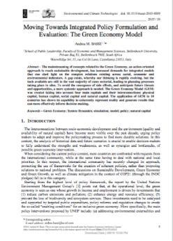
72 Mur Mur SEB of Climate Information Services Climate impacts from different scenarios accumulate over time The reference scenario (green line) serves to assess added benefits and avoided costs The difference between the reference and CIS scenarios are benefits obtained from CIS Cumulative Additional Cost For Reestablishing The Road Network 20 B Cumulative Economic Loss From Livestock Due To Extreme Weather 200 M 15 B 150 M 10 B 100 M 5 B 50 M Time (Year) Cumulative Additional Cost For Reestablishing The Road Network : WISER SEB CIS 19 Mar - CIS Investment Cumulative Additional Cost For Reestablishing The Road Network : WISER SEB CIS 19 Mar - BAU Cumulative Additional Cost For Reestablishing The Road Network : WISER SEB CIS 23 Jan - Reference Time (Year) Cumulative Economic Loss From Livestock Due To Extreme Weather : WISER SEB CIS 19 Mar - CIS Investment Cumulative Economic Loss From Livestock Due To Extreme Weather : WISER SEB CIS 19 Mar - BAU Cumulative Economic Loss From Livestock Due To Extreme Weather : WISER SEB CIS 23 Jan - Reference

73 SEB of CIS: Cost benefit ratio Example results for 30% and 100% coverage Scenario Reference (0% CIS coverage) Full climate impacts BAU (30% CIS coverage) Impacts climate CIS investment (100% coverage by 2035) CIS investment Total impacts (million USD) 9' Total SEBs (million USD) Total investment (million USD) Cost to benefit ratio ' ' ' '

74 Quality control: Validation of results The obtained simulation results were validated based on Results obtained from the analysis of the dataset Comparison of simulation results to the range of impacts obtained from data analysis International reports Assessment of whether the combined induced impacts produced by the model are conform with publications on climate impacts in Africa Peer reviewed papers

75 Limitations (1) Use of average data obtained from a dataset covering 8 African countries Customization of the tool to a country context requires more specific data, such as Share of area affected Local price assumptions on agriculture produce, livestock, roads, health care, etc. Impacts of adverse weather are estimated on monthly precipitation Main cause of floods are dry spells followed by 2-3 days of heavy rain

76 Limitations (2) High level of aggregation for the assessment of impacts Some impacts might be caused by a combination of factors, and require more detailed causal relationships At this stage, investments in CIS are based on a fraction of GDP, not on specific costs of interventions

77 Summary The model captures social, economic and environmental dynamics Including climate variations in the analysis has cascading effects through all sectors The performance of the system changes depending on the climate assumptions used Policy effectiveness has to be assessed using a variety of indicators, across sectors, actors, over time and space

78 Thank you! For more information you can find me at: KnowlEdge Srl