SHORT MEDIUM LONG. Lifetime growth pattern and beef eating quality. ( Growth Path ) FINAL REPORT

Transcription

1 SHORT MEDIUM LONG Lifetime growth pattern and beef eating quality ( Growth Path ) FINAL REPORT May 2016 AHDB Beef & Lamb (Project Number: 72510) Prepared by: Dr Jimmy Hyslop 1, Dr Carol-Anne Duthie 1, Dr Ian Richardson 2, Dr John Rooke 1, Mr Dave Ross 1. 1 SAC Consulting and SRUC, Kings Buildings, Edinburgh EH9 3JG 2 Division of Food & Animal Science, University of Bristol, Langford, Bristol BS40 5DU Prepared for: Kim Matthews, AHDB Beef & Lamb, Stoneleigh Park, Warwickshire 1

2 Contents Page 1 Executive summary and recommendations 3 2 Members of the Growth Path project management team 4 3 List of Tables 4 4 List of Figures 5 5 Introduction & Background 6 6 Project Objectives 7 7 Materials & Methods 8 8 Results 8.1 Live animal growth performance Slaughter & carcass characteristics Beef eating quality measurements Economic analysis measurements 33 9 Discussion 9.1 Alternative growth paths, live animal performance 38 and carcass outputs 9.2 Alternative growth paths and beef eating quality Economic consequences of alternative growth paths 40 and production systems 10 Conclusions Knowledge exchange activities References Appendices 47 2

3 1 Executive summary and recommendations The objectives of this three year project were to investigate the relationships between three alternative lifetime growth paths and any effects on live animals performance, carcass quality, beef eating quality and economic performance parameters when either short, medium or long term finishing systems are used to finish steer or heifer beef cattle. The trial design was a 3 x 2 factorial continuous design experiment with three finishing systems or growth paths (GP) and two sexes of finishing cattle (steers and heifers). A total of 72 Limousin crossbred (LIMx) cattle of suckler herd origin were used (12 steers & 12 heifers) for each of the three GPs and started the trial at approximately 12 months of age. The short duration GP animals were finished indoors on an intensive concentrate based finishing system and slaughtered at months of age. The medium duration GP animals were turned out to graze a high quality grass reseed from months of age and finished indoors during the subsequent winter feeding period when offered a mixed forage:concentrate (F:C) finishing diet. They were slaughtered at months of age when judged to have achieved commercially acceptable carcass characteristics (target R4L). Finally, the long duration GP animals were grazed for two summer periods on poor quality, unimproved grassland with the intervening winter period being a store period where the animals were offered forage based diets. The final finishing diet was a mixed F:C diet offered during their 2 nd winter prior to slaughter at months of age. All animals completed their respective GPs as planned. Average days on trial were 86, 286 and 622 (P<0.001) for the short, medium and long duration GPs respectively with mean slaughter ages of 15.1, 21.8 and 32.9 (P<0.001) months. Similarly, mean slaughter liveweights were 528, 624 and 671 kg (P<0.001) and average lifetime daily liveweight gains were 1.58, 0.96 and 0.54 kg/d (P<0.001) respectively. Mean carcass weights were 298, 356 and 378 kg (P<0.001) with average slice shear force measurements of 10.8, 10.4 and 11.9 kg (P<0.05) for the short, medium and long GPs respectively indicating that the long GP finishing systems produced beef of poorer tenderness than either the short or medium GP systems. The proportional content of gristle in the striploin section samples was also significantly higher (P<0.001) in the long GP system at values of 1.63, 1.62 and 1.96 % of the longissimus dorsi muscle respectively. Human taste panel assessments of beef eating quality showed increased levels of toughness (38.7, 42.5 & 46.9; P<0.05) between the short, medium and long GPs respectively. Despite these differences, the long GP system could still produce beef eating quality parameters that were considered acceptable for the human food chain. From a financial perspective, the average total feeders margin ( /head) was 301, 523 and 570 (P<0.001) for the short, medium and long GP systems respectively. Despite this however, when these values were expressed on a daily basis (i.e. total FM/days on the GP system) the mean values were 3.72, 1.86 and 0.91 ( /head/day) across the same three GP systems. Once variable costs were deducted, Gross Margin figures were 36, 86 and 65 /head whilst further deducting fixed cost estimates reduced Net Margin figures to -27, -34 and -209 /head for the short, medium and long GP systems respectively. Total variable costs were 265, 437 and 505 /head whilst estimated fixed costs were 63, 120 and 274 /head for the short, medium and long GP systems respectively. Examining the quadratic relationships between feeders margin and the costs incurred either here or from industry estimates revealed that the greatest potential for profit was to be found when animals were slaughtered at younger, rather than older ages. It is concluded that commercial beef finishers be advised to adopt efficient, short to medium duration (12-20 months) finishing systems that deliver higher quality beef to the human food chain whilst offering producers the greatest opportunity for commercial profit. 3

4 2 Members of the Growth Path project management team 2.1 SAC Consulting Ltd Dr Jimmy Hyslop 2.2 SRUC Beef & Sheep Research Centre Dr Carol-Anne Duthie Dr John Rooke Mr Dave Ross 2.3 Bristol University Dr Ian Richardson 2.4 AHDB Beef & Lamb Mr Kim Matthews Dr Mary Vickers 3 List of Tables Table 1. Description of the growth paths and LIMx cattle used in this study Table 2. Feed analysis for the housed periods during the short, medium and long duration finishing systems Table 3. TMR composition for the housed periods during the short, medium and long duration finishing systems Table 4. Days on trial, age, liveweight and overall daily liveweight gain parameters for steers and heifers managed using alternative growth path finishing systems Table 5. Slaughter and carcass parameters for steers and heifers managed using alternative growth path finishing systems Table 6. Meat quality parameters and meat weights for steers and heifers managed using alternative growth path finishing systems 4

5 Table 7. Joint weights and proportional contents for steers and heifers managed using alternative growth path finishing systems Table 8. Sensory taste panel meat eating quality scores for steers and heifers managed using alternative growth path finishing systems Table 9. Prediction of gristle weight from areas (mm 2 ) taken from digital photographs of carcasses at the 5 th and 10 th rib section ends Table 10. Sale price, sale values, store values and feeders margins for steers and heifers managed using alternative growth path finishing systems Table 11. Financial analysis of system margins and some physical quantities used for steers and heifers managed using alternative growth path finishing systems 4 List of Figures Figure 1. Outline of the three growth path management systems of short, medium and long duration along with number and timing of animal slaughter and fixed cost assumptions per day. Figure 2. Grass availability (kg DM/ha) measured using a rising plate meter Figure 3. Stocking rate (LSU/ha) for cattle in 2013 and 2014 Figure 4. 5 th 10 th rib joint section removed at the abattoir showing loin and gristle areas estimated at the 10 th rib Figure 5. Steer & heifer LW (kg) and LWG (kg/d) for cattle during various indoor & outdoor periods during each of the short, medium and long finishing periods Figure 6. Quadratic relationships between slaughter age and slaughter liveweight (A), daily liveweight gain (B) and cold carcass weight (C). Figure 7. Quadratic relationships between slaughter age and Slice Shear Force (A), Cooking Loss (B) and Gristle:Joint Weight (C). Figure 8. Quadratic relationships between slaughter age and Total Feeders Margin (A), Daily Feeders Margin (B) and Daily Feeders Margin and Average Costs (C). 5

6 5 Introduction & Background AHDB Beef & Lamb (AHDB B&L) have recently identified the importance of the relationships between lifetime growth pattern (which is influenced by the production system) and beef eating quality and their influence on the environment with regard to Greenhouse Gas emissions and profitability. One key aspect of these complex interrelationships, which requires detailed investigation within a properly balanced experiment, is the relationships between lifetime growth patterns associated with alternative production systems on-farm and the effect of these variable growth patterns on consumer perceptions of beef eating quality. Recent changes to the AHDB B&L quality standard means that both clean steers and heifers up to 36 months of age can obtain the quality mark for beef. However, some debate remains as to the effects that alternative patterns of growth over the lifetime of the animal may have on carcass and meat eating quality parameters. To further inform this debate, this study comprises a dedicated experiment using 36 steers and 36 heifers of comparable status and known genetics, managed to achieve different lifetime growth paths with a consequent wide range in slaughter age, but using production systems that are typical of commercial practice on UK farms. As well as growth patterns throughout the growing and finishing periods of the animals alternate production cycles, this study will also provide information on the carcass and eating quality characteristics of this range of animal types and production systems. Background It is a long-standing assumption that the eating qualities of beef declines as animals get older with tenderness getting worse as animals age in particular (Berry et al, 1974; Carroll, et al, 1976). There is evidence from the literature to support this with regard to a very broad range in age of beef cattle at slaughter from veal calves to mature cows (Bouton, et al, 1981), possibly related to the collagen content of the muscle (Lepetit, 2008). However, with regard to the age range at which clean cattle are usually slaughtered within the UK beef market (typically months of age) the situation is much less clear cut. Some evidence does exist that variation in growth rate may affect muscle structures, enzymatic activities and composition (Oddy et al, 2001). Fishell, et al. (1985) report a positive association between pre-slaughter growth rate and tenderness with faster growing animals being judged more tender by a trained taste panel. When fed a high energy diet, Aberle, et al, (1981) suggested that growth rate immediately before slaughter may be a more important determinant of meat tenderness than length of time animals were offered a high energy diet pre-slaughter. In support of these implications that higher growth rate result in more tender beef, Thompson et al, (1999) found a weak but positive correlation (r=0.23) between palatability score and growth rate. Subsequent analysis of a similar Australian dataset indicated that the most consistent relationship was an increase in palatability of the striploin with increased growth rate during the finishing phase of the production system with a lesser effect seen when growth rate during backgrounding was considered (Perry and Thompson, 2005). In his review of managing meat tenderness, Thompson (2002) 6

7 reports a curvilinear relationship between finishing growth rate and palatability which appeared to plateau at a growth rate of approximately 1.2 kg/day. Whilst he suggests that any growth rate effects on beef tenderness may be relatively small, it remains a critical control point for the production sector of the beef supply chain. Alternatively, some authors have concluded that growth rate per se has little effect on beef eating quality (Sinclair, et al, 2001) or muscle fibre characteristics (Maltin et al, 2001) under UK systems of production. Other studies have pointed to the more complex relationships which may arise from variable growth rate over the period from weaning to slaughter. Allingham et al, (1998) suggests that animals who have experienced periods of compensatory growth following periods of nutrient restriction may exhibit altered connective tissue characteristics which may in turn affect meat tenderness. Conversely, Bruce et al, (1991) report that meat tenderness measured by shear force, appeared to be primarily affected by energy intake pre-slaughter and intramuscular fat content rather than rate of compensatory growth. Purchas et al, (2002) reports that an increase in age of between 8 to 10 months may be associated with less tender beef for cattle finished on pasture. In contrast, Barton (2012) reports that older animals had higher tenderness scores (more tender) compared with animals slaughtered at an age approximately 4 months younger (i.e. 18 months rather than 14 months of age). This confusing picture from the scientific literature with often conflicting research reports, suggest several underlying observations can be made:- a) many factors will interact to determine the meat eating qualities and tenderness scores of any particular animal within any particular production system b) it is not clear where the critical points are with regard to growth rates, age at slaughter or lifetime growth path trajectories for UK cattle types c) considerable debate will remain across the industry until UK based studies address these issues using production systems typical of those found on commercial farms This short summary of some of the available information in this area has highlighted the need for a long term UK based beef production study focussed on examining the relationships between alternative lifetime growth paths and eating quality in an attempt to improve the eating experience associated with UK beef. 6 Project Objectives 6.1 The three main objectives of this project were to: Produce finished steers and heifers at a wide range of ages between months of age according to alternative lifetime growth patterns which 7

8 included a period of growth check for the older animals using typical production systems used on-farm throughout the Britain Evaluate effects of lifetime growth patterns on overall productive output, carcass and meat eating quality parameters (particularly including toughness attributes) assessed by both laboratory and trained taste panel methods Communicate the results to AHDB B&L, the wider farming community and associated industry practitioners. 7 Materials & Methods 7.1 Establishment phase The over-arching study design was a 3 x 2 factorial, continuous design experiment examining three alternative growth paths in two sexes of LIMx finishing cattle. The experiment was established and conducted at the SRUC Beef Research Centre, just south of Edinburgh during the spring of 2013 and continued until the last animals were slaughtered in March The three alternative growth paths were characterised principally by the duration of the finishing system. The short duration system slaughtered all animals between 12 and 16 months of age; the medium duration system slaughtered all animals between 18 and 24 months of age and the long duration system slaughtered all animals between 28 and 36 months of age. Diets, grazing regimes and management of each of these growth path groups is described below. All of the LIMx steer and 6 of the LIMx heifer animals used in the experiment were bred from the SRUC Limousin and Aberdeen Angus 2-breed reciprocal cross herd on the unit whilst the remaining heifers were purchased from commercial suckler herds with Limousin sires that were known. Both steers and heifers were allocated to alternative growth path groups taking individual sire into account so that no one sire dominated within any one group for either steers or heifers. This ensured no confounding sire effects across alternative growth path management regimes. The full description and composition of the alternative groups are detailed in Table 1 and the management outline of each group along with the assumed fixed cost per day for each of the management periods is shown in Figure 1:- Table 1. Description of the growth paths and LIMx cattle used in this study Age range LIMx Growth path at slaughter Steers Heifers Spares Total Short duration of each sex 26 Medium duration Long duration

9 Figure 1. Outline of the three growth path management systems of short, medium and long duration along with number and timing of animal slaughter and fixed cost assumptions per day. On average, cattle were on trial for 86, 286 and 622 days for the short, medium and long GP systems respectively. They were actually on farm an additional 47 days as a transitional/quarantine phase before the trial started on 1 st May Age at slaughter averaged 15.1, 21.8 and 32.9 months of age whilst actual slaughter ages ranged from 12 to 35 months for individual animals as planned. The start LW was higher for animals on the short GP system due to the late start of the trial at approximately 12 months of age rather than an earlier start of this finishing treatment that would be encountered in commercial practice. Had we not done this, these animals would have been very underweight at slaughter, especially the heifers. Ideally, all animals would have been started on treatment at an earlier stage of life, possibly at weaning at approximately 7 months of age or even younger. Practical constraints made this impossible here. All indoor diets were offered as total mixed rations (TMR) through a Keenan Feeder Wagon fitted with the PACE feed recording system. Short duration finishing system all animals remained indoors from the trial start on 1 st May 2013 on straw bedded courts and were fed a barley beef type, high concentrate diet until sent for slaughter. The TMR diet comprised barley (BAR), rapeseed meal (RSM), straw (STR), molasses (MOL) and minerals (MIN) as shown below. Both steers and heifers were sent for slaughter in three groups during June, July and August respectively. Medium duration finishing system all animals were turned out to grass on 13 th of May due to the cold weather during the late spring of 2013 delaying the growth of grass. Normally, cattle would be out to grass anything up to 6 weeks earlier than this had the weather been more typical. The grass sward was a 2 year old perennial ryegrass reseed that 9

10 was well established and of good grazing quality (see pictures below). Grass was fertilised on 3 occasions during the summer of 2013 with a total of 125 kg of nitrogen/ha. Grass availability (kg DM/ha) was assessed at fortnightly intervals using a rising plate meter (Jenquip, 2009) and stocking rate was adjusted at periodic intervals to ensure that a minimum of 1500 kg/ha of grass DM was available to animals at all times. Stocking rates were adjusted by altering the area of grass available to the animals. Medium term animals were housed on 9 th October 2013 and offered a forage based TMR on an ad libitum basis until sent for slaughter in three batches during November 2013, January 2014 and April 2014 respectively. All medium group animals were housed in a single straw bedded pen and the TMR comprised wholecrop barley (WCB), grass silage (SIL), BAR, RSM, MOL and MIN as shown below. Long duration finishing system - all animals were turned out to grass on 13 th of May 2013 for their 1 st grazing period as for the medium group except that they were grazed on an old unimproved grassland pasture that only received 50 kg/ha of nitrogen fertiliser in spring and was judged to be of poor grazing quality (see pictures below). Grass availability was assessed as for the medium group and grass availability was maintained above 1500 kg/ha of grass DM at all times. Stocking rates were again altered when required by altering the area of similar grassland available to the animals. Animals were housed on 9 th October 2013 for their 1 st winter store period and remained in the same straw bedded pen until turnout the following spring on 2 nd April Two winter store TMR diets were offered. The first comprised SIL, STR and MIN and was offered during November Jan whilst the 2 nd TMR comprised WCB, SIL, BAR, RSM and MIN and was offered during February until April At turnout for their 2 nd summer at grass, animals returned to the same area of unimproved grassland which was managed in the same way until housing again on 15 th October These long group animals were then housed together in a single straw bedded pen and offered a forage based TMR on an ad libitum basis until sent for slaughter in three batches during November 2014, January 2015 and March 2015 respectively. The TMR comprised wholecrop barley (WCB), grass silage (SIL), BAR, RSM, MOL and MIN as shown below. SHORT MEDIUM LONG 10

11 7.2 Feed analysis and grassland measurements For all indoor feeding periods, the oven DM contents of individual feed components were determined on duplicate samples twice weekly and bulked feed samples were collated on a monthly basis for subsequent laboratory analysis. These bulked feed samples were analysed for DM, ash, crude protein (CP), acid detergent fibre (ADF), neutral detergent fibre (NDF), acid hydrolysis ether extract (AHEE), and starch (Ministry of Agriculture Fisheries and Food, 1992) and gross energy (GE) by adiabatic bomb calorimetry. The chemical composition of individual dietary ingredients are shown in Table 2 whilst the TMR composition of the experimental diets as recorded using the diet software on the complete diet feeder wagon (Keenan 140) and using the oven DM figures taken twice weekly are given with the TMR chemical composition in Table 3. Table 2. Feed analysis for the housed periods during the short, medium and long duration finishing systems g/kg DM unless otherwise stated g/kg MJ/kg DM DM ASH CP ADF NDF AHEE STA GE ME Short duration BAR RSM STR Medium duration SIL WCB BAR RSM Long duration SIL 2013/14 (as per SIL for medium duration) WCB 2014 (as per WCB for medium duration) STR 2013/ SIL 2014/ BAR MDG SIL: grass silage; WCB: wholecrop barley silage; STR: barley straw; BAR: barley grain; RSM: rapeseed meal; MDG: maize dark grains; MOL: molasses; MIN: minerals DM: dry matter; ASH: non-organic matter; CP: crude protein; ADF: acid detergent fibre; NDF: neutral detergent fibre; AHEE: acid hydrolysis ether extract; STA: starch; GE: gross energy; ME: metabolisable energy. MOL contained 704, 706 and 718 g/kg DM and the MIN contained 974, 977 and 961 g/kg DM in the short, medium and long duration systems respectively. The MIN supplement contained (mg/kg): Fe, 6036; Mn, 2200; Zn, 2600; Iodine, 200; Co, 90; Cu, 2500; Se, 30: (µg/kg): vitamin E, 2000; vitamin B12, 1000; vitamin A, 1515; vitamin D,

12 Table 3. TMR composition for the housed periods during the short, medium and long duration finishing systems TMR composition (g/kg DM) SIL WCB STR BAR RSM MDG MOL MIN Short duration finishing TMR Medium duration finishing TMR Long duration store TMR Long duration store TMR Long duration finishing TMR TMR chemical analysis g/kg DM unless otherwise stated g/kg MJ/kg DM DM ASH CP ADF NDF AHEE STA GE ME Short duration Finishing TMR Medium duration Finishing TMR Long duration Store TMR 1 Long duration Store TMR 2 Long duration Finishing TMR see table 2 for abbreviations. Chemical analysis of concentrate feedstuffs was generally in line with published values (MAFF, 1992) and forage quality was generally good with grass silage ME contents ranging from reflecting the fact that they were both 1 st cut samples and that the swards used were recently reseeded and well fertilised. The WCB used in both the medium and long diets during the 2013/14 winter was lower in ME at 10.0 MJ/kg DM but was fairly high in CP at 101 g/kg DM compared with published values (MAFF, 1992). The short duration total mixed ration (TMR) was comprised of only concentrates and straw and its analysis figures reflected this fact with an ME of 12.2 MJ/kg DM and a CP of 132 g/kg DM. In contrast, the finishing TMRs used for the medium and long finishing system 12

13 were both mixed forage:concentrate diets but still of reasonably high quality with ME contents of MJ/kg DM and CP contents of 139 and 140 g/kg DM respectively. The store diet used for the long duration animals during their 1 st winter of 2013/14 were of lower quality with ME contents ranging from and CP contents of g/kg DM reflecting the lower levels of animal performance expected from these animals during this period. As described above, grass growth has been measured using a rising plate meter in both the medium and long pastures in 2013 and in the long term pasture during the grazing phase in The grass availability throughout the grazing season on these pastures is shown in Figure 2 whilst the stocking rates (LSU/ha) are shown in Figure 3. During both 2013 and 2014 (long) the grass availability remained in excess of the minimum requirement of 1500 kg/ha for both the medium and long groups. Turnout for the long group was achieved much earlier in 2014 with grass DM availability at the minimum 1500 kg/ha early in April rather than well into May in Consequently, the long duration animals were turned out to grass much earlier in 2014 in early April rather than the later turnout date for both the medium and long groups on 13 th May during the very late spring of Figure 2. Grass availability (kg DM/ha) measured using a rising plate meter 13

14 Figure 3. Stocking rate (LSU/ha) for cattle in 2013 and Live animal growth performance measurements From the start of the trial period on 1 st May 2013 until slaughter each animal from all groups was weighed on a fortnightly basis to allow calculation of daily liveweight gain (DLWG) values during each relevant period of the study. Estimates of DLWG was obtained over slightly different periods for each of the three GP systems as appropriate and according to the relevant periods of management for each group of animals. DLWG for the short duration animals was estimated very simply as one estimate from the start of the feeding period on 1 st May 2013 until slaughter on average 86 days later. For both the medium and long duration GP groups DLWG estimates were obtained for an early summer and a late summer grazing period as appropriate along with an estimate of the DLWG loss that occurred as a result of gut fill losses during the short period following turnout for both groups and for the gut fill increases that occurred following the housing period for the long GP group. DLWG during the winter feeding periods prior to slaughter for both the medium and long groups were calculated once across the whole period to facilitate GP group averages across the three slaughter dates for each group. Finally, the overall average DLWG across the entire periods from start (1/5/13) to slaughter (various periods across groups) was calculated to allow an overall comparison of mean growth rates for each animal in each GP group. 14

15 7.4 Slaughter & carcass measurements Within each of the growth path groups both steers and heifers remained within the same pens and on the same diets from the start of their respective housing periods until sent for slaughter. Animals were slaughtered in three batches per growth path group as described above for the short, medium and long duration finishing systems respectively. On the day before slaughter, ultrasonic fat depth (FD) and muscle depth (MD) at the 12 th /13 th rib was measured in all animals. For all animals ultrasound measurements of FD and MD were obtained at the 12 th /13 th rib using an industry standard Aloka 500 machine (BCF Technology Ltd, Livingston, Scotland, UK). Images were analysed using Matrox Inspector 8 software (Matrox video and Imaging Technology Europe Ltd, Middlesex, UK) to obtain the individual FD and MD values. Steers and heifers were selected for slaughter based on BW and visual assessment of fatness. The animals were transported (approximately 1 h) to a commercial abattoir and slaughtered within 2 h of arrival. Cattle were stunned using a captive bolt, exsanguinated and subject to low voltage electrical stimulation. Following hide removal, carcasses were split in half down the mid-line and dressed to UK specification (see Meat and Livestock Commercial Services Limited beef authentication manual, www. mlcsl.co.uk, for full description). As well as cold carcass weights (CCW) being commercially reported, EUROP conformation and fat classifications (Fisher, 2007), based on the UK scale, were allocated to all carcasses through visual assessment using a trained assessor. Fat and conformation grades were subsequently expressed on a 15 point scale according to Kempster et al, 1984 to allow statistical analysis of the results. Killing out proportions (KO) were also calculated from CCW and LW at slaughter to allow comparisons across both the GP and animals sex experimental factors. 7.5 Beef eating quality measurements Removal of 5 th 10 th rib section was undertaken at 48 hours post slaughter in the abattoir using standard butchery techniques. After removal and the collection of digital images for gristle prediction (see below), all rib sections were vacuum-packed and delivered to Bristol University using chilled transport where they were analysed for IMF and SSF before the remainder was frozen and stored at -18 o C until the end of the entire trial when all 72 animals were available for sensory taste panel analysis. Gristle prediction using digital images at the abattoir A further objective of the project was to gather pictorial images of the gristle component at the quartering point in the abattoir to establish whether an in-abattoir image acquired on the loin cross-section, could provide an estimate of the gristle weight as measured by dissection. A 2592 by 1944 pixel colour image of the loin and surrounding tissue cross sections was taken using a standard digital camera at 5 th and 10 th rib loin dissection positions, as 5 th rib sections of the loin were removed from the carcass at 2 days post-mortem for subsequent meat quality work. 15

16 Pictorial images were calibrated using a standard protocol, by immediately taking an image of a calibration sheet placed on the target loin surface. Images were then dimensionally corrected using Matrox Inspector software. This software was also used to manually segregate total loin area (mm 2 ) and visible gristle areas (cumulative mm 2 ). Both the 5 th rib section and 10 th rib ends of the loin sections were analysed. A typical 10 th rib cross section with annotated gristle is shown in Figure 4 below. The data obtained were used to assess whether there is a relationship between loin and gristle areas and total gristle weight as measured by carcass dissection. Actual gristle weights were determined by joint dissection at Bristol University as part of the meat analysis work. Figure 4. 5 th 10 th rib joint section removed at the abattoir showing loin and gristle areas estimated at the 10 th rib Loin area Gristle areas 16

17 Fatty acid analyses and slice shear force measurements For intra-muscular fat (IMF) analysis, freeze dried samples of steak were first trimmed of outer fat, gristle and connective tissue. Total fat was then extracted from the muscle with o C petrol ether in a Buchi unit. For ease of presentation, total IMF results are reported simply as a percentage of wet tissue weight (IMF %). Slice shear force (SSF) was determined on each individual cooked steak (Shakelford et al, 1999). Two by 20mm long steaks from each animal were cooked to an internal temperature of 71 o C using a clam shell grill on the high heat setting. Once cooking was complete, cooking loss was determined (weight reduction on cooking). A cut was then made across the width of the longissimus dorsi (sirloin) at a point about 10 to 20 mm from the lateral end of the muscle and then a second cut was made using a sample sizing box across the width of the longissimus, parallel to and at a distance of 50 mm from the first cut. This created a 50 mm long section from the lateral end of the longissimus with muscle fibres orientated at a 45 o angle. This 50 mm long section was placed in a slice box and centred on two 45 o slots with the angle of the slots lined up with the muscle fibre angle and two parallel cuts simultaneously made through the length of the 50 mm long section. This cut provides a 10 mm thick, 50 mm long slice that is parallel to the muscle fibres. The SSF measurement is a measure of the force (expressed here in kg) that is required for a simulated knife blade to cut through a 10 x 50 mm cross section slice parallel to the fibre axis using an XT/AT analyser. It was possible to obtain 1-2 samples for each of the cooked steaks from each of the 72 animals and the 3-4 values obtained are reported as mean values. Sensory taste panel assessment undertaken at Bristol University Sensory analysis was carried out by a 10-person trained taste panel (BSI, 1993). The samples were defrosted overnight at 4 C and then cut into steaks 20 mm thick. Steaks were grilled to an internal temperature of 74 C in the geometric centre of the steak (measured by a thermocouple probe). All fat and connective tissue were then trimmed and the muscle was cut into blocks of 2 cm 3. The blocks were wrapped in pre-labelled foil, placed in a heated incubator and then given to the assessors in a random order chosen by a random number generator. Assessors are asked to rate the samples on eight point category scales (Appendix A) for texture, juiciness, flavour intensity (higher values denote more favourable responses), abnormal flavour intensity (lower values denote more favourable responses). Two additional hedonic questions relating to flavour liking and overall liking are also used. An additional set of descriptors were used to assess aspects of beef texture profiles on cutting, chewing, eating and on a residue basis, all on a 100 mm scale (Appendix B). All live animal performance, carcass quality and meat eating quality parameters have been analysed using the ANOVA facility in Genstat 16 to assess the main treatment effects (GP and animal sex). In selected instances the quadratic relationships between slaughter age and key parameters have been quantified using Microsoft excel. 17

18 7.6 Economic analysis measurements As part of the overall evaluation of alternative growth path management systems, a full Gross and Net Margin calculation has been undertaken for each of the three growth paths studied (short, medium & long) and where possible for each of the animal sexes used (steer & heifers). The statistical significance of these main treatment factors along with their major interactions has been assessed using the ANOVA facility in Genstat 16. As with the physical parameters above, the quadratic relationships between slaughter age and key parameters have been quantified using Microsoft excel in certain instances. Approaches taken to calculate profitability and economic analysis In all alternative growth path systems, the actual variable costs incurred from the start of the experiment on 1 st May 2013 until slaughter for all animals reaching the end of the trial have been used to calculate the financial performance up to the Gross Margin stage. In contrast, the fixed costs at a research unit such as the Beef and Sheep Research Centre (BSRC) are atypical and unrepresentative of most farming situations. Consequently, the average fixed costs for the winter feeding periods from both the AHDB Beef and Lamb Stocktake Report and the QMS Cattle and Sheep Enterprise Profitability in Scotland report have been assumed and applied to the actual Gross Margin figures obtained to calculate a Net Margin figure. In addition, an average fixed cost of 0.20 per head per day has been assumed for the summer grazing period in all relevant cases to cover labour (e.g. checking animals), machinery (e.g. transport etc) and other fixed costs (e.g. fencing repairs) whilst animals are outdoors at grass. Fixed costs from the 2014 & 2015 Stocktake Reports (AHDB, 2014 & 2015) and the 2014 & 2015 editions of the QMS publication Cattle and Sheep Enterprise Profitability in Scotland (QMS, 2014 & 2015) have been used since at the time of calculation, they are the most recent figures available that relate to the duration of the experiment which ran from Gross Margin calculations Actual sale prices on a CCW basis (p/kg CCW) and total sale values ( /head) were obtained from the commercial abattoir where all cattle were slaughtered. In both years an initial Feeders Margin was calculated on both a /head basis and a /head/day basis. This feeder s margin was simply the difference between the sale value of the animals obtained from the abattoir and the store value of the animal at the start of the trial period. The store value was calculated using the BW at the start and the average price per kg BW paid for the animals when they had been purchased a few weeks earlier. Where animals were home bred then the average price for the value of the animals purchased was assumed to apply also to home bred animals of the same breed/sex type or estimated from QMS price reports during the period the animals were purchased. The next stage in the financial calculations was to calculate total feed costs from the actual feed usage figures during the relevant housing periods from the start to slaughter obtained using the SRUC Beef and Sheep Research Centre data-sets. These data sets in this instance 18

19 were not individual feed intake data but simply total feed distributions from the TMR feeder wagon (Keenan 140) to each pen where both the steer and heifer animals for each GP under study were housed. It is important to acknowledge here that this simply provides an estimate of average feed usage for the pen as a whole and does not represent individual variation in daily feed intake per animal. Any animal to animal variation in feed usage used to calculate the average values reported here simply reflects the difference between animals in the number of days each animal received the diets in question. Total feed usage throughout the housed feeding periods were then calculated and the total feed cost per tonne of complete diet DM applied to these total feed usage figures to obtain a total feed cost on a /head basis. Margin over Feed and Forage (MOFF) figures on a /head basis were then calculated. Estimates of straw bedding material usage (2.3 kg/head/day) was combined with its purchase price and days on trial for each animal to calculate a bedding cost along with a Margin over Feed, Forage and Bedding (MOFFB) figure, again on a /head basis. Other variable costs were then assessed and included vet and medical costs ( 3.40 /head for 1 respiratory vaccination), a haulage charge at 28 /head in 2013 or 19 /head in 2014 & 2015, an abattoir killing charge at /head, a levy payment at 4.20 /head and a livestock sundries charge assumed to be 1 /head to cover items such as replacement tags. Since the farm had its own borehole, no water charges were included. Each of these figures did actually apply or were assumed to apply to each steer and heifer on trial. Total variable costs were then calculated and subtracted from the Feeders Margin to give a Gross Margin figure on a /head basis for each animal. Net Margin calculations Following the Gross Margin calculation, an average fixed cost daily rate was assumed from figures published by both AHDB Beef and Lamb and QMS for both 2014 & 2015 as noted above. These daily fixed cost rates cover labour, buildings, machinery, land and capital costs associated with various classes of beef finishing business surveyed by these respective organisations each year. A total of six categories of beef finishing business ranging from short duration, mainly concentrate fed systems to longer term, mainly forage fed enterprises were included in the datasets yielding these figures. The average daily fixed cost rate was 0.73 /head/day across the reported systems for the 2013 summer and the winter period whilst it was 0.86 /head/day for the winter. As listed in Figure 1 and above, the summer fixed cost rate was estimated at 0.20 /head/day during both summer periods. These fixed cost figures were then applied along with the number of days from start of the trial (1/5/13) to slaughter to calculate a total fixed cost figure for each animal on trial on a /head basis. A Net Margin or profit figure was then calculated for each animal as the difference between the Gross Margin and fixed cost figures, again expressed on a /head basis. 19

20 8 Results All the animals from the short-term, medium-term and long-term finishing growth path groups completed their finishing phases and were slaughtered in 3 batches per growth path group as planned. A summary of their overall growth and slaughter performance along with the major eating quality parameters and economic analysis are given in the tables and graphs below. Some additional data (detailed taste panel texture profile scores) has been presented in Appendix C in order to ease overall data presentation. 8.1 Live animal growth performance Average LW and DLWG for each of the steer and heifer groups have been depicted graphically for key periods in Figure 5 below. The original intention was to turnout the cattle on the 1 st of May 2013 and take this date as the common start date for all groups in the trial. However, the very late spring and poor grass growth meant that turnout had to be delayed until 13 th May for both the medium and long duration groups. Both the medium and long duration groups exhibited an expected drop in LW immediately following turnout due to changes in gut fill as their diet changed from silage and concentrate to spring grass (average decline across all animals was approximately 18 kg (~5 %) during the 9 days after turnout). Similar drops in LW following turnout in 2014 were seen with the long GP cattle. This gut fill effect should always be borne in mind when looking at grazing growth rates on-farm and comparing them with results produced in research experiments where these changeover effects are almost always excluded from reported performance figures. As a consequence of these gut fill effects following turnout, early season growth rates have been expressed after this initial gut fill change has been accounted for. As can be seen from Figure 5, when managed on the housed system using intensive concentrate based diets the short GP steers grew at approximately 1.7 kg/d whilst the heifers grew at approximately 1.4 kg/d, typical of intensive barley beef type diets (see Nutribeef report). Whilst early season growth rates were reasonably high at 1.2 kg/d for both steers and heifers on the medium GP system, they only grew at an average of 0.8 kg/d over the whole summer when managed on good quality grass. This is because late summer growth rates were poor at approximately 0.40 kg/d for both sexes. Once these medium GP cattle were offered a mixed forage:concentrate finishing diet during housing there DLWG improved to 1.63 and 1.29 kg/d for steers and heifers respectively. The situation when cattle were managed on poor quality grass during the long GP system resulted in even poorer growth performance. Growth rates at kg/d were a little better during the 1 st half of the 2013 summer compared with the 2 nd half ( kg/d), again presumably as a result of grass quality. Consequently, overall growth rates during the 2013 summer months were as low as kg/d on average for cattle managed on poor grassland typical of these long duration finishing systems. A similar pattern of good early season, but poor late season growth rates were seen during 2014 such that overall summer growth rates during the 2014 grazing season were 0.28 and 0.24 kg/d for steers and heifers respectively. Growth rates during the final finishing winter were kg/d where a higher quality finishing diet was offered. In general and as planned, this long GP system was characterised by periods of reasonable DLWG but also several periods of poor DLWG or even periods of liveweight loss. 20

21 Figure 5. Steer & heifer LW (kg) and LWG (kg/d) for cattle during various indoor & outdoor periods during each of the short, medium and long finishing periods 21

22 The fact that transitional periods of LW loss occurred in two years at turnout on the long GP compared with the medium GP system also resulted in a more divergent growth pattern across systems. No such periods of divergent growth pattern occurred for the short GP system. Days on trial for each respective growth path finishing strategy, age at slaughter, LWs and overall DLWGs for the whole trial period are given in Table 4. On average cattle were on trial for 86, 286 and 622 days for the short, medium and long GP systems respectively. They were actually on farm an additional 47 days as a transitional/quarantine phase before the trial started on 1 st May Age at slaughter averaged 15.1, 21.8 and 32.9 months of age whilst actual slaughter ages ranged from 12 to 35 months for individual animals as planned. Average slaughter LWs were 528, 624 and 671 kg whilst average DLWGs over the entire trial periods were 1.58, 0.96 and 0.54 kg/d for the short, medium and long duration finishing systems respectively. These differences in age, slaughter LW and DLWG were all highly significantly different between GP groups (P<0.001). Despite being very similar in ages throughout, heifers were generally lighter (slaughter LW 658 vs 558 for steers and heifers respectively) and grew more slowly than steers (1.12 vs 0.94 for steers and heifers respectively) as might be expected (P<0.001). In general, there were significant interactions between sex and GP system with effects often being more pronounced in heifers than steers (e.g. in factors such as age at slaughter and slaughter LW). Simple quadratic relationships between age at slaughter and three key parameters (slaughter LW, DLWG and cold carcass weight (CCW)) are shown in Figure 6. In general it can be seen that whilst slaughter LW and CCW did increase progressively over time the rate and extent of increase declined as the animals approached the months slaughter age period. DLWG figures declined progressively with slaughter age as might be expected. The R 2 values for these simple quadratic relationships explained between % of the variation in these key performance parameters indicating that choice of GP or finishing system has a very important influence on the magnitude of these parameters in commercial practice. 8.2 Slaughter & carcass characteristics As well as the increase in slaughter LW noted above, there were also some differences in carcass characteristics between GP systems as detailed in Table 5. CCW also increased significantly (P<0.001) at 298, 356 and 378 kg across the short, medium and long GP systems respectively. In particular, steer fat and muscle depths were generally higher on the medium GP system, perhaps reflecting the 50% concentrate component of the winter finishing diets for these animals. Average fat depths were 7, 11 and 9 mm whilst the mean muscle depth figures were 74, 78 and 82 mm for the short, medium and long GP systems respectively. In contrast, the pre-slaughter fat and muscle depths for the short GP diet were lower, particularly for the heifers on this system. This may have been a reflection of the low carcass weight for these animals, possibly reflecting the fact that the heifers in particular may have been under-finished. Killing out proportion did not vary across GP or sex and averaged 565 g/kg. Converting the fat and conformation gradings from the abattoir to a 15 point scale for statistical analysis revealed lower values for the heifers managed on the short GP system although this was only significant for the fat scores. 22

23 Table 4. Days on trial, age, liveweight and overall daily liveweight gain parameters for steers and heifers managed using alternative growth path finishing systems Sig. of effects Parameter Short Medium Long Sex GP Sex GPxSex Days on trial (Steers) 81 a 271 b 610 c 321 *** *** (Heifers) 90 a 300 b 635 c a 286 b 622 c 331 s.e.d. Growth Path = 14.2; Sex = 11.6; GPxSex = 20.1 slaughter (Steers) 468 a 655 b 997 c 707 *** *** (Days) (Heifers) 450 a 670 b 1003 c a 663 b 1000 c 707 s.e.d. Growth Path = 15.0; Sex = 12.3; GPxSex = 21.2 slaughter (Steers) 15.4 a 21.5 b 32.8 c 23.2 *** *** (Months) (Heifers) 14.8 a 22.0 b 33.0 c a 21.8 b 32.9 c 23.3 s.e.d. Growth Path = 0.49; Sex = 0.40; GPxSex = 0.70 Start LW (1/5/13) (Steers) 472 a 381 b 355 b 403 a *** *** * (kg) (Heifers) 345 c 317 c 316 c 326 b 408 a 349 b 335 b 364 s.e.d. Growth Path = 11.8; Sex = 9.7; GPxSex = 16.8 Slaughter LW (Steers) 592 a 670 b 712 c 658 a *** *** * (kg) (Heifers) 465 d 579 a 631 e 558 b 528 a 624 b 671 c 608 s.e.d. Growth Path = 11.3; Sex = 9.2; GPxSex = 15.9 DLWG (on trial) (Steers) 1.72 a 1.05 c 0.58 e 1.12 a *** *** ** (kg/d) (Heifers) 1.43 b 0.88 d 0.50 e 0.94 b 1.58 a 0.96 b 0.54 c 1.03 s.e.d. Growth Path = 0.040; Sex = 0.034; GPxSex = values within experimental factors not sharing common superscripts differ significantly (P<0.05). 23

24 Figure 6. Quadratic relationships between slaughter age and slaughter liveweight (A), daily liveweight gain (B) and cold carcass weight (C). (A) Slaughter Liveweight vs Slaughter Age (B) Daily Liveweight Gain vs Slaughter Age (C) Cold Carcass Weight vs Slaughter Age 24

25 Table 5. Slaughter and carcass parameters for steers and heifers managed using alternative growth path finishing systems Sig. of effects Parameter Short Medium Long Sex GP Sex GPxSex Slaughter LW (Steers) 592 a 670 b 712 c 658 a *** *** * (kg) (Heifers) 465 d 579 a 631 e 558 b 528 a 624 b 671 c 608 s.e.d. Growth Path = 11.3; Sex = 9.2; GPxSex = 15.9 Fat depth (Steers) 8 ab 11 b 8 a 9 * * (mm) (Heifers) 6 a 11 b 9 ab 9 7 a 11 b 9 ab 9 s.e.d. Growth Path = 1.2; Sex = 1.0; GPxSex = 1.8 Muscle depth (Steers) 76 ab 77 ab 86 c 78 * * (mm) (Heifers) 71 a 79 bc 77 ab a 78 ab 82 b 78 s.e.d. Growth Path = 2.6; Sex = 2.0; GPxSex = 3.8 Cold carcass wt (Steers) 337 bc 384 d 398 d 373 a *** *** * (kg) (Heifers) 258 a 328 b 359 c 315 b 298 a 356 b 378 c 344 s.e.d. Growth Path = 8.2; Sex = 6.7; GPxSex = 11.6 Killing Out (Steers) (g/kg) (Heifers) s.e.d. Growth Path = 6.4; Sex = 5.2; GPxSex = 12.9 Fat score (1-15 ) (Steers) 7.62 a 7.50 a 7.38 a 7.50 * (Heifers) 5.88 b 8.12 a 7.75 a a 7.81 b 7.56 ab 7.38 s.e.d. Growth Path = 0.505; Sex = 0.412; GPxSex = Conf score (1-15 ) (Steers) (Heifers) s.e.d. Growth Path = 0.461; Sex = 0.376; GPxSex = values within experimental factors not sharing common superscripts differ significantly (P<0.05). 25

26 8.3 Beef eating quality measurements Physical beef eating quality and 5 th rib meat weight parameters are shown in Table 6. In a similar way to the fat depth and fat score values, the IMF % was significantly higher (P<0.01) at 2.84% in the medium GP system compared to the short (1.78%) or the long (1.80%) GP finishing system. The mechanical measure of beef tenderness represented by SSF was significantly higher (P<0.05) in beef produced by the long GP finishing system. Values were 10.8, 10.4 and 11.0 kg force for the short, medium and long GP system respectively. Similarly, cooking loss % was significantly higher (P<0.01) for the long GP system with values being 24.8, 26.4 and 29.1 % across the short, medium and long systems respectively. The total 5 th rib joint weight and the weight of bone in that joint reflected the differences in carcass weights overall with significantly heavier (P<0.001) steer (8616 g) compared to heifer (7693 g) total joint weights. Differences between GP finishing systems significantly increased (P<0.05) between the short to medium GP systems, particularly for heifers. However, despite the numerical values being higher again for the long GP system, no further significant increase was apparent. Total 5 th rib joint weight values were 7042, 8646 and 8776 g across the short, medium and long GP systems respectively. Weights of longissimus dorsi muscle and gristle weights (g) along with some 5 th rib joint percentages are given in Table 7. As might be expected, longissimus dorsi weights reflected carcass weights with values being 1600, 1950 and 2085 g for the short, medium and long GP systems respectively. Significant differences (P<0.001) only existed between the short and medium GPs but not the long duration GP finishing system. Conversely, gristle weights increased significantly (P<0.001) across all GP systems with values being 25.8, 31.5 and 40.2 g across the short, medium and long systems respectively. Overall, gristle weight represented only a small percentage of either the total 5 th rib weight (0.4%) or the longissimus dorsi weight (1.74%). However, as a % of the 5 th rib joint weight, gristle % ranged across 0.37, 0.36 and 0.46 % and from 1.63, 1.62 and 1.96 % of the longissimus dorsi weight across the short, medium and long GP finishing systems respectively. No significant differences were seen in the % of total 5 th rib joint weight represented by the longissimus dorsi proportion with an average value of 23%. Simple quadratic relationships between age at slaughter and three key beef eating quality parameters (SSF, cooking loss % and gristle:joint weight (%)) are shown in Figure 7. In general it can be seen that whilst age at slaughter did increase SSF for the long GP system, the overall increase was numerically small and the quadratic relationships only explained between and 0.04 of the total variation in the dataset for the steers and heifers respectively. A similar picture was evident for the quadratic relationships between age at slaughter and cooking loss % and gristle:joint %. The R 2 values for these simple quadratic relationships explained approximately only 0.20 and 0.30 of the variation in these key beef eating quality parameters respectively. This suggests that beef eating quality parameters are likely to be influenced by factors beyond the effect of age at slaughter where alternate GP or finishing systems are used in commercial practice to a considerable extent. 26

27 Table 6. Meat quality parameters and meat weights for steers and heifers managed using alternative growth path finishing systems Sig. of effects Parameter Short Medium Long Sex GP Sex GPxSex Moisture content (Steers) (%) (Heifers) s.e.d. Growth Path = 0.32; Sex = 0.26; GPxSex = 0.45 IMF (%) (Steers) 1.97 ab 3.03 c 1.65 a 2.22 ** * (Heifers) 1.59 a 2.65 bc 1.95 ab a 2.84 b 1.80 a 2.14 s.e.d. Growth Path = 0.322; Sex = 0.263; GPxSex = Slice shear force (Steers) 10.6 a 10.2 a 12.2 b 11.0 * * (kg) (Heifers) 10.9 ab 10.7 ab 11.8 ab a 10.4 a 11.9 b 11.0 s.e.d. Growth Path = 0.54; Sex = 0.53; GPxSex = 0.67 Cooking Loss (Steers) 24.9 a 26.4 ab 28.3 bc 26.5 ** * (%) (Heifers) 24.6 a 26.5 ab 30.0 c a 26.4 a 29.1 b 26.8 s.e.d. Growth Path = 0.93; Sex = 0.76; GPxSex = 1.32 Joint weight (g) (Steers) 7846 b 8980 c 9023 c 8616 a *** *** * (Heifers) 6238 a 8311 b 8529 b 7693 b 7042 a 8646 b 8776 b 8155 s.e.d. Growth Path = 295.8; Sex = 241.5; GPxSex = Bone weight (g) (Steers) 2170 bc 2388 cd 2421 d 2326 a * *** * (Heifers) 1739 a 1999 b 2125 b 1954 b 1954 a 2193 b 2273 b 2140 s.e.d. Growth Path = 81.9; Sex = 66.9; GPxSex = values within experimental factors not sharing common superscripts differ significantly (P<0.05). 27

28 Table 7. Joint weights and proportional contents for steers and heifers managed using alternative growth path finishing systems Sig. of effects Parameter Short Medium Long Sex GP Sex GPxSex L. dorsi weight (Steers) 1734 b 2018 c 2055 c 1936 *** * (g) (Heifers) 1466 a 1882 bc 2115 a a 1950 b 2085 b 1879 s.e.d. Growth Path = 92.4; Sex = 75.4; GPxSex = Gristle weight (Steers) 28.6 b 35.1 c 42.7 d 35.5 a *** *** * (g) (Heifers) 23.0 a 27.8 b 37.8 c 29.5 b 25.8 a 31.5 b 40.2 c 32.5 s.e.d. Growth Path = 1.51; Sex = 1.24; GPxSex = 2.14 Bone:Joint wt (Steers) 27.5 a 26.9 a 26.9 a 27.1 a ** ** * (%) (Heifers) 27.8 a 24.1 b 25.0 b 25.6 b 27.7 a 25.5 b 25.9 b 26.4 s.e.d. Growth Path = 0.64; Sex = 0.52; GPxSex = 0.90 L dorsi:joint wt (Steers) 22.2 a 22.5 ab 22.8 ab 22.5 * (%) (Heifers) 23.2 ab 22.7 ab 24.8 b s.e.d. Growth Path = 0.82; Sex = 0.67; GPxSex = 1.16 Gristle:L dorsi wt (Steers) 1.65 ab 1.75 b 2.10 c 1.83 a *** ** * (%) (Heifers) 1.61 ab 1.49 a 1.82 b 1.64 b 1.63 a 1.62 a 1.96 b 1.74 s.e.d. Growth Path = 0.080; Sex = 0.065; GPxSex = Gristle:Joint wt (Steers) 0.37 a 0.39 a 0.48 b 0.41 *** * (%) (Heifers) 0.37 a 0.34 a 0.45 b a 0.36 a 0.46 b 0.40 s.e.d. Growth Path = 0.019; Sex = 0.015; GPxSex = values within experimental factors not sharing common superscripts differ significantly (P<0.05). 28

29 Figure 7. Quadratic relationships between slaughter age and Slice Shear Force (A), Cooking Loss (B) and Gristle:Joint Weight (C). (A) Slice Shear Force vs Slaughter Age (B) Cooking Loss vs Slaughter Age (C) Gristle:Joint Weight vs Slaughter Age 29

30 The main beef eating quality scores on an 8 point scale from the human taste panel at Bristol University are shown in Table 8. Generally, beef from steers was tougher at a scale value of 44.4 than beef from heifers at a scale value of 41.0 (P<0.05). Steer beef also had a significantly (P<0.01) lower overall liking value at 42.3 compared to heifers beef at Average toughness values were 38.7, 42.5 and 46.9 for the short, medium and long GP finishing systems with significant differences (P<0.05) between all GP groups of animals on average. Examining the significant (P<0.05) interaction however, revealed that these group differences were all associated with the steer animals whereas no significant increase in heifers values was apparent. Juiciness was unaffected by either sex or GP system. Beef flavour values averaged 44.4, 47.2 and 46.6 across the small, medium and long GP systems and was unaffected by sex. Only the difference between the short and medium GP group was statistically significant (P<0.05) although in this case it was due to a slightly greater effect in the heifers rather than the steers. Mean abnormal flavour values were 23.7, 20.6 and 19.7 for the short, medium and long GP systems with only the short values being statistically significantly higher (P<0.05) than the other two groups. Again the difference was greater (P<0.05) in the heifers than in the steers. Of the two hedonic values, GP finishing system increased flavour liking (P<0.01) in the medium and long GP systems compared to the short GP system with mean values of 43.8, 47.4 and 47.8 across the three GP systems respectively. Heifers were again most responsible (P<0.05) for this effect rather than steers. Finally, average overall liking values were 42.4, 45.4 and 44.2 for the short, medium and long GP finishing system with the medium group being significantly higher (P<0.05) than the short GP group only. Additional taste panel texture profile scores are given in Appendix C. Similar general trends in the data are apparent with regard to toughness on both cutting and eating, ease of cutting, beef moisture content on eating and chewiness on eating. Generally the beef from the longer GP finishing systems was regarded as tougher than beef from the short GP system and steers were generally tougher than heifers. Very few effects were seen in the residue parameters studied. Table 9 contains the main results from the statistical assessment of digital images in the abattoir and their relationship with gristle weights as measured by dissection. Very high auto-correlations were seen between the potential predictor variable derived by adding both the 5 th and 10 th rib images together and their individual component values as would be expected. However, this does mean that where the combined values are used as a predictor variable (i.e. 5 th & 10 th rib values added together), then neither of the individual component values can be used alongside. As can be seen from Table 9, the best single predictor of gristle weight was indeed the 5 th & 10 th rib gristle area measurement added together. It explained approximately 43% (R 2 of 0.428) of the variation in gristle weight (i.e. size, or in this case area, and weight really do help to explain each other). Deriving additional predictor variables by mathematical transformation in various guises and then searching for multiple regression equations to predict gristle weight did improve the best available prediction equation slightly to an R 2 of However, this did have to include both gristle and loin area estimation from the digital images rather than just gristle area on its own. 30

31 Table 8. Sensory taste panel meat eating quality scores for steers and heifers managed using alternative growth path finishing systems Sig. of effects Parameter Short Medium Long Sex GP Sex GPxSex Toughness (Steers) 39.0 a 42.7 a 51.7 b 44.4 a * * * (8 point scale) (Heifers) 38.5 a 42.4 a 42.1 a 41.0 b 38.7 a 42.5 b 46.9 c 42.7 s.e.d. Growth Path = 1.60; Sex = 1.32; GPxSex = 2.24 Juiciness (Steers) (8 point scale) (Heifers) s.e.d. Growth Path = 1.38; Sex = 1.13; GPxSex = 1.93 Beef Flavour (Steers) 43.9 a 45.2 ab 46.8 ab 45.3 * * (8 point scale) (Heifers) 44.9 a 49.2 b 46.4 ab a 47.2 b 46.6 ab 46.1 s.e.d. Growth Path = 1.03; Sex = 0.85; GPxSex = 1.45 Abnormal Flavour (Steers) 23.2 a 20.8 ab 19.8 b 21.3 * * (8 point scale) (Heifers) 24.2 a 20.3 b 19.6 b a 20.6 b 19.7 b 21.3 s.e.d. Growth Path = 1.24; Sex = 1.05; GPxSex = 1.75 Hedonic Flavour liking (Steers) 43.1 a 46.0 ab 47.7 ab 45.6 ** * (8 point scale) (Heifers) 44.4 ab 48.9 b 47.9 ab a 47.4 b 47.8 b 46.6 s.e.d. Growth Path = 1.33; Sex = 1.10; GPxSex = 1.87 Overall liking (Steers) 40.8 a 43.8 ab 42.3 ab 42.3 a * ** * (8 point scale) (Heifers) 44.1 ab 47.1 b 46.1 b 45.8 b 42.4 a 45.4 b 44.2 ab 44.1 s.e.d. Growth Path = 1.27; Sex = 1.04; GPxSex = 1.79 values within experimental factors not sharing common superscripts differ significantly (P<0.05). 31

32 Table 9. Prediction of gristle weight from areas (mm 2 ) taken from digital photographs of carcasses at the 5 th and 10 th rib section ends Correlation matrix between potential predictor variables from digital area (mm 2 ) estimates (1) (2) (3) (4) (5) (6) % Gristle area 5 th Rib (1) % Loin area 5 th Rib (2) 0.25 % Gristle area 10 th Rib (3) % Loin area 10 th Rib (4) % Gristle area (5 th & 10 th ) Rib (5) % Loin area (5 th & 10 th ) Rib (6) Best single predictor of gristle weight (g) Gristle weight (g) = 12.33(+/- 2.84) (+/ ) x Gristle area (5 th & 10 th ) Rib R 2 = 0.428: RSD = Best multiple regression predictor of gristle weight (g) Gristle weight (g) = (+/- 7.27) (+/ ) x Gristle area (5 th & 10 th ) Rib (+/ ) x Loin area 5 th Rib R 2 = 0.497: RSD =

33 8.4 Economic analysis measurements Financial analysis of the results up to the Feeders Margin stage where we have real individual animal values available is given in Table 10 whilst the mean values for the three GP systems overall up to the Gross and Net Margin stages is given in Table 11. As already mentioned we do not have individual feed intake data so these reported differences between GP systems in Table 10 do not represent true animal to animal variation. Sale price values were higher for steers than heifers on a p/ kg CCW basis probably reflecting the slightly higher carcass weights and to a lesser extent, better carcass grades. However, the biggest effect here (P<0.001) was between GP systems with the short GP group appearing to have the highest price/kg CCW. Of course this is not a true comparison since these animals from different GP groups were sold at different points in time so these GP differences simply reflect the changing market prices for beef across these various commercial timeframes. Whilst sale values reflect similar timeframe bound changes to price levels, they also contain real variation due to real differences in carcass size and quality across the GP and sex trial factors. Store values in Table 10 reflect the relative LW of the animals at the start of the trial period (1 st May 2013). The higher store values for the steers on the short GP system reflect their slightly higher LW at that time (see Table 4). Feeders Margin (FM) on both a /head and /head/day basis were higher (P<0.05) for steers compared to heifers with mean values of /steer and /heifer respectively. The comparable daily values for FM were 2.43/steer and 1.90/heifer. Average FM ( /head) were , and for the short, medium and long GP finishing systems respectively. These averages were significantly different (P<0.01) across all GP groups but more significantly (P<0.01) influenced by heifers than steers. However, once these animal totals had been divided by the number of days on trial (86, 286 and 622 for the short, medium and long GP groups respectively) an alternative pattern emerged. Mean FM values on a /head/day basis were 3.72, 1.86 and 0.91 for the short, medium and long GP systems respectively, this time more heavily influenced by steers (P<0.05) rather than heifers. Whilst FM progressively increased on a /head basis as age at slaughter increased; the reverse was true and FM progressively declined as age at slaughter increased when expressed on a /head/day basis. Table 10 also shows the full financial analysis of the three GP finishing systems to both a GM and NM stage. Since no individual animal estimates of feed or straw usage are available, nor any split between the sexes; only the GP comparison can be detailed here. Initially, the average amount of feed DM consumed whilst animals on each GP system were housed indoors and amounts of straw bedding used are given. These figures include the 2013 summer housing period for the short GP finishing system, the winter finishing period for the medium GP system and both the winter store and winter finishing periods for the long GP system. Estimates of feed DM consumed were 582, 1381 and 2392 kg/head and straw bedding usage were 197, 409 and 879 kg/head for the short, medium and long GP systems respectively. All these differences between GP systems were highly significantly different (P<0.001). 33

34 Along with estimates of pre-trial and grazing costs, total costs of feed consumed whilst indoors were deducted from the FM figures to give a MOFF of 94, 162 and 176 /head across the short medium and long GP finishing systems. Further deducting bedding costs and other variable costs resulted in GM figures of 36, 86 and 65 /head for the short medium and long systems respectively. When added together the total variable costs were 265, 437 and 505 /head across the short, medium and long systems and statistical analysis showed significance (P<0.05) between all three GP finishing systems. Total fixed costs were estimated at 63, 120 and 274 /head across the GP systems and total costs when both variable and fixed costs were added together were 328, 557 and 779 /head. All of these differences in cost estimates between the alternative GP finishing systems were highly significantly different (P<0.001). Subtracting the projected fixed costs from the Gross Margin figures gives Net Margin figures of -27, -34 and -209 /head across the short, medium and long GP finishing systems respectively with the difference between the long GP systems and the shorter duration finishing systems being highly significant (P<0.001). Simple quadratic relationships between age at slaughter and three key financial margin parameters (total FM { /head}, daily FM { /head/day} and daily feeder s margin plus SRUC and average industry total costs { /head/day}) are shown in Figure 8. For FM on a /head basis, it can be seen that whilst age at slaughter did progressively increase FM for the longer GP system, the overall increase/months of age diminished as animals reached months old. The nature of the quadratic relationships suggests that there is likely to be little difference on average between FM/head between an animal slaughtered at either 25 or 35 months of age. When expressed on a /head/day basis, it is evident that a quadratic decline in FM/day exists as age at slaughter progresses. Once again it is clear that there is likely to be little difference in FM/day for animals slaughtered at ages between 25 and 35 months of age. In addition, it is of critical importance that the level of FM during this month of age period is below 1/head/day. The final graph in Figure 8 again depict FM on a /head/day basis but here the total production costs have been added again on a /head/day basis. Firstly, the total production costs from the study conducted here have been added as the red horizontal line. This includes all variable and fixed costs as does the green lines which represent the same total production costs but this time taken from published values reported the both the AHDB Stocktake and QMS industry surveys as describe above. The cost lines are flat within GP finishing system since only average values are available from industry publications and also from this study because no individual animal feed intake figures are available. The interpretation from the graph is that only those individual animals whose FM figures are above these cost lines have made a positive Net Margin (i.e. only these animals have made a profit). It is clear from the graph that it is only some of the animals at the short duration to early medium duration end of the spectrum that have made a profit. Animals at the longer duration or greater age end of the finishing spectrum have all made a loss. 34

35 Table 10. Sale price, sale values, store values and feeders margins for steers and heifers managed using alternative growth path finishing systems Sig. of effects Parameter Short Medium Long Sex GP Sex GPxSex Sale price (Steers) a bc d *** * * (p/kg CCW) (Heifers) ab c d a b c s.e.d. Growth Path = 3.81; Sex = 3.11; GPxSex = 5.39 Sale value (Steers) 1374 a 1505 b 1475 b 1451 a *** *** * ( /head) (Heifers) 1038 c 1256 d 1335 a 1210 b 1206 a 1380 b 1405 b 1331 s.e.d. Growth Path = 26.6; Sex = 21.7; GPxSex = 37.6 Store value (Steers) 1033 a 937 b 912 b 961 a * *** * ( /head) (Heifers) 776 c 777 c 758 c 770 b 905 a 857 b 835 b 866 s.e.d. Growth Path = 26.8; Sex = 21.9; GPxSex = 38.0 Feeders Margin (Steers) ab c c a ** * * ( /head) (Heifers) a b c b a b c s.e.d. Growth Path = 33.88; Sex = 27.66; GPxSex = Feeders Margin (Steers) 4.32 a 2.07 c 0.91 d 2.43 a *** *** * ( /head/d) (Heifers) 3.12 b 1.66 d 0.91 d 1.90 b 3.72 a 1.86 b 0.91 c 2.17 s.e.d. Growth Path = 0.205; Sex = 0.167; GPxSex = values within experimental factors not sharing common superscripts differ significantly (P<0.05). 35

36 Table 11. Financial analysis of system margins and some physical quantities used for steers and heifers managed using alternative growth path finishing systems Parameter Short Medium Long sed Sig. Physical quantities used Total feed DM consumed a 1381 b 2392 c *** whilst indoors (kg DM) Straw bedding (kg) 197 a 409 b 879 c 45.7 *** Financial parameters Feeders Margin ( /head) 301 a 523 b 570 b 40.3 *** Pre-trial cost Grazing cost Feed cost indoors a 271 b 328 c 25.5 * MOFF 94 a 162 b 176 b 33.8 * Bedding cost 23 a 35 b 70 b 3.8 *** MOFFB Other Var Costs Total Var Costs 265 a 437 b 505 c 29.6 * GROSS MARGIN Total Fixed Costs 63 a 120 b 274 c 10.9 *** Total Costs 328 a 557 b 779 c 40.3 *** NET MARGIN -27 a -34 a -209 b 38.3 *** 1 Does not include grazing DM intake 2 Dietary costs: ( /t DM): Short finishing TMR: ; Medium finishing TMR: ; Long finishing TMR: ; Long store TMR 1: ; Long store TMR 2: Other Var. Costs are: Vet & Med, haulage (both variable between animals), abattoir killing charge ( 11.60/h), levies (QMS /h), livestock sundries ( 1/h). 36

37 Figure 8. Quadratic relationships between slaughter age and Total Feeders Margin (A), Daily Feeders Margin (B) and Daily Feeders Margin and Average Costs (C). (A) Total Feeders Margin vs Slaughter Age ( /head) (B) Daily Feeders Margin vs Slaughter Age ( /head/day) (C) Daily Feeders Margin and Average Costs vs Slaughter Age ( /head/day) 37

38 9 Discussion A number of general points are worthy of note with regard to the results obtained. The start LW was higher for animals on the short GP system due to the relatively late start of the trial where animals were approximately 12 months of age rather than an earlier start of this finishing treatment at approximately 7-8 months of age that would be encountered in commercial practice. Had we not done this, these animals would have been very underweight at slaughter, especially the heifers. Ideally, all animals would have been started on treatment at an earlier stage of life, possibly at weaning at approximately 7 months of age or even younger. Practical constraints made this impossible here. Were this study to be repeated, we would recommend starting the animal management regimes at weaning (6-8 months of age for suckler bred animals) at the latest. Since feed accounts for approximately 70% of total variable costs in beef finishing systems, caution must be used when considering the financial figures reported here since no actual feed intake parameters on an individual animal basis were measured at any point during this study. Whilst pen based data from electronic recording of feed distribution from TMR feeders can provide interesting, useful and highly relevant information to commercial producers, it should not be viewed with the same degree of statistical rigour that would be provided by individual animal feed intake data. Variation between the GP treatments here relating to variable costs; (feed in particular), reflect difference in days on trial rather than real variance between individual animals. 9.1 Alternative growth paths, live animal performance and carcass outputs One key feature that the consideration of different growth paths has established is the potential of the LIMx animals used in this study to grow. These typically commercial LIMx animals have the capacity to grow well in excess of 1.6 kg/day (steers) and in excess of 1.4 kg/d (heifers) as can be seen in the short duration GP group shown in Figure 4. This is consistent with other LIMx animals used at SRUC in recent years (see the Nutribeef report). Whilst both steers and heifers grew at approximately 1.2 kg/d on the good quality grass reseeds for the 1 st half of the summer in the medium duration system, growth rates were much poorer at 0.4 kg/d during the 2 nd half of the summer. This resulted in average summer growth rates of approximately 0.8 kg/d which is little better than half the growth rate of the animals kept on an indoor system. This overall growth rate illustrates the poor quality of grass during the 2 nd half of the summer. However, this is typical of practical reality on most beef cattle farms. It is clear that spending a summer at grass is little better than managing these cattle on a store type of diet. Not necessarily the best practice for finishing beef cattle efficiently and profitably. It is true to point out that these cattle on the medium duration system here were managed on a set stocking continuous grazing system which lends itself to declines in grass quality in late summer and consequently poorer growth. Adopting strategies to improve the quality of grassland management, its utilisation and animal performance could improve this situation in commercial practice. These improved grazing techniques could include rotational grazing, paddock grazing or even strip grazing approaches. However, it is important to consider that animal performance is unlikely to improve in the 1 st half of the summer, especially when the drop in LW due to gut fill changes following turnout is considered. This leaves only 38

39 improved growth in late summer as the mechanism to improve overall growth and profitability. Even if this could be achieved in most cases it is unlikely that animals would finish on a grass diet alone without any form of supplementary feeding and then would still require to be housed before finishing and incur most or even all of the costs that have been incurred by keeping them indoors on the short duration system anyway. The long duration system of grassland management with poor quality grassland produced even worse animal performance figures at grass with average growth rates in both years never exceeded 0.37 kg/day over the whole summer period. This is approximately ¼ of the growth potential that these animals have exhibited when managed on the short duration finishing system. Again, grassland management could be improved beyond the set stocking approach used here but the poor nature of this type of grassland would severely limit the scope to achieve finishing levels of performance in these animals. Farmers are attracted to finishing cattle at grass because of the perceived cheapness of grass as a feed. However, where animal growth is inhibited at grass, its apparent cheapness may not necessarily lead to a profitable system of production overall. Despite these reservations about finishing animal performance at grass it must be acknowledged that slaughter weights and carcass outputs were lower for the short GP finishing system here, partly perhaps at least because we were not able to start this finishing system management at a younger age than 12 months. Many farmers may see this reduced output and therefore sale value as a major limitation to making profit. Others may also point to the risk of under finishing heifers on the short GP system, as was certainly the case here. The low fat scores for heifers on the GP system in Table 5 are evidence of that. However, these concerns and risks may be less of an issue today compared to the recent past given market moves to penalise overly large carcasses and better reward those cattle within the kg CCW bracket. In summary, the effects of these alternative GP finishing systems on animal performance can be described in relation to the age at slaughter of the animal, the time taken to manage the animal on the GP system and to produce the carcass and the overall growth rates achieved throughout the finishing periods spent on the system. Short GP animals were 15.1 months of age at slaughter, spent 86 days on the system and grew on average at 1.58 kg/d. Medium GP animals were 21.8 months of age at slaughter, spent 286 days on the system and grew on average at 0.96 kg/d. Long GP animals were 32.9 months of age at slaughter, spent 622 days on the system and grew on average at 0.54 kg/d. 9.2 Alternative growth paths and beef eating quality Whilst a considerable number of individual assessments of beef eating quality were made, a number of key features have emerged consistently across the measurement techniques employed. Firstly, tenderness (measured mechanically by SSF) and toughness (reported by the human taste panel) were both significantly poorer for the animals (mainly steers) managed on the long duration GP system. This may have been a result of either, animal age per se, or as a result of the intermittent growth patterns of the long duration GP animals where periods of 39

40 little or no growth may have led to changes in muscle deposition and/or composition leading to less tender beef. It is impossible to say which of these factors is the most instrumental in this regard from the study conducted here. However, the overall result seems clear. Long duration finishing systems are likely to produce tougher or less tender beef compared to shorter duration finishing systems. It should be noted however, that all the beef produced here was well within normal ranges considered acceptable by the consumer. For example, all the SSF measurements were below 18 kg force across all animals in this study (Figure 7). One further feature is the observation that age at slaughter only explained 20% of the variation in SSF (Figure 7). This strongly suggests that many other factors will affect beef tenderness beyond merely how old they are. This fact may go a long way to help explain why there are conflicting reports in the scientific literature with regard to the relationship between tenderness and age described in the background discussion above. Analysis of the gristle component of the 5 th 10 th rib joint section tends to compliment the picture regarding beef tenderness/toughness outlined above. Gristle as a % of both the whole joint section and the longissimus dorsi muscle significantly increased in the long duration GP animals (again mainly steers). This may also adversely affect the consumer s perception of beef from these animals. However, it must be acknowledged that overall gristle represented only a small % of the total joint weight. In addition, the results of the overall liking category of assessment by the taste panel suggests that these trained consumers at least, found the beef from these older animals just as acceptable overall as beef from their younger counterparts. One of the objectives here was to examine the possibility of using digital images of the gristle component of beef carcasses as a means of predicting true gristle weights in the carcass. Some success in the approach used here was achieved such that actual gristle weight (g) could be predicted with an accuracy approaching 50% (R 2 = 0.497; Table 9). Further scientific study would likely improve this accuracy still further across a wider dataset of individual animals. However, an issue of wider importance is highlighted by the fact that gristle makes up such a small proportion of the overall joint section studied (0.4 %). Before further study in this area is contemplated it should be assessed whether spending levy payers money to improve this accuracy of predicting such a small component of the carcass would yield a value for money return on investment to either levy payers or indeed provide much scope to enhance the consumers beef eating experience. Careful consideration of these and related questions (e.g. are there areas of the carcass where gristle could be studied and represents a higher proportion of the sample tested so that its influence could be more informative). 9.3 Economic consequences of alternative growth paths and production systems One of the confounding features of a study like this when it comes to financial considerations is the fact that changes in prices and financial values over time will influence the results as well as differences between the treatment regimes under study. As well as the changed prices mentioned above contributing to the differences in prices and sale values between the three 40

41 GP finishing systems noted above, changes in input prices can act in a similar way. For example, it can be seen in Figure 8 that the SRUC costs for the short duration GP system are considerably above the average industry costs also shown on the graph. This is because the industry costs are an average of two countries over two years whereas the SRUC costs relate only to one year when the short duration GP cattle were finished. This just happened to be 2013 when barley prices were approximately 200/t. This factor also influenced the differential between the GP systems because in 2014 and 2015 barley prices were at a much more normalised range at /t. However, in this case it should be borne in mind that this did not enhance the profitability of the short duration GP system in relation to the others. In fact, the cost effect was in the opposite direction, although the carcass sale price was the other way round. With regard to the medium and long grassland based finishing systems, whilst the variable costs on a daily basis may seem low for these longer duration systems; it is difficult to see how the poor animal performance (DLWG) can justify low variable costs along with the inevitable high fixed costs that accompany these systems. In addition, from an overall farm business point of view where a breeding herd is also on the farm, overall cow numbers and therefore calf output would be reduced with these long duration systems since finishing cattle are grazing grass that would be better utilised by cows and calves. Management and business profit is all about exploiting the fixed costs resources to best effect and finding a way to optimise financial output per unit fixed cost. Long duration finishing systems do not lend themselves to generating profit from grassland based suckler beef production. They use a large amount of fixed resources for some very inefficient levels of animal performance overall throughout the lifetime of these animals. Consideration of the financial figures in totality has highlighted a number of key areas. Firstly it is clear that in profitable beef finishing systems, the time it takes to get an animal from weaning/purchase to slaughter is of critical importance and one of the main drivers of profit. Whilst increased days may seem to lead to increased sale value, the increased costs associated with those extra days outweighs the increased value such that overall profit declines. Secondly, both the usefulness and limitations of Feeders Margin as a mechanism for farmers to evaluate the profitability of beef finishing systems and individual animals needs to be more widely understood. Thirdly, all costs including all variable and all fixed costs must be taken into account fully when assessing the profitability of alternative growth path finishing systems. Finally, consideration of the Feeders Margin and costs graph in Figure 8 should emphasise that beef finishers must concentrate on those animals and systems where profit potential does exist if they are to prosper in a marketplace that is less reliant on subsidy and derives more profit from the commercial value and cost relationships involved. In summary, the effects of these alternative GP finishing systems on GP system financial performance can be described in relation to the age at slaughter of the animal, the time taken to manage the animal on the GP system and to produce the Net Margin or Profit resulting from the finishing times spent on the system. Short GP animals were 15.1 months of age at slaughter, spent 86 days on the system and produced a Net Margin of. -27/head. Medium GP animals were 21.8 months of age at slaughter, spent 286 days on the system and produced a Net Margin of -34/head. Long GP animals were 32.9 months of age at slaughter, spent 622 days on the system and produced a Net Margin of -209/head. 41

42 10 Conclusions Short and medium duration finishing systems result in growth paths to slaughter with relatively consistent patterns of positive growth throughout, whereas long duration finishing systems may result in growth paths with periods of slow or even negative growth on an intermittent basis. Acceptable carcasses can be produced using short, medium or long duration finishing systems although carcass weight may be lighter where short duration systems are used unless finishing diets are introduced as early as possible in the production cycle. Short, medium and long duration finishing systems can produce beef that is acceptable to the consumer but long duration systems may result in beef being slightly tougher and having a slightly higher gristle content compared to shorter finishing systems. Financial margin may be greater at the Feeders Margin level on a /head basis where finishing systems are of long duration and carcass weights are high. However, once both higher variable and higher fixed costs are taken into account then Net Margin or profit levels are likely to be lower where longer duration finishing systems are used. Commercial beef finishers should be advised to adopt efficient, short to medium duration finishing systems that will deliver higher eating quality beef to the human food chain whilst offering producers the greatest opportunity for commercial profit. 11 Knowledge exchange activities It was agreed at an initial project meeting during 2013 that the majority of the project KE activity would occur during the later stages of the project when results become available. As well as opportunities for project management staff (including AHDB B&L staff) to visit the work underway during project management meetings, there were also 3 occasions when other AHDB B&L visitors attended the BSRC to see the work of this project on-going. A small group of AHDB staff visited in June 2013 and another group in November 2013 along with a small group of farmer clients. The AHDB R&D committee also visited in January Following further discussion it was also agreed that SAC staff (Dr Jimmy Hyslop) would engage in KT activities in England during the last week in January 2016 along with AHDB B&L staff (Dr Mary Vickers) when results from this project and the Nutribeef project were discussed in full with a wide range of farmer audiences. A total of five meetings were held in Cornwall, Gloucestershire, Northamptonshire, Staffordshire and Yorkshire with in excess of 50 beef farmers attending each meeting. One future opportunity for KE activity has been identified on 13 th September 2016 on behalf of AHDB B&L staff (Dr Liz Genever). 42

43 12 References Aberle, E.D., Reeves, E.S., Judge, M.D., Hunsley, R.E. and Perry, T.W. (1981). Palatability and muscle characteristics of cattle with controlled weight gain: time on a high energy diet. Journal of Animal Science, 52(7): p Allingham, P.G., Harper, G.S. and Hunter, R.A. (1998). Effect of growth path on the tenderness of the semitendinosus muscle of Brahman-cross steers. Meat Science, 48: p Berry, B.W., Smith, G.C. and Carpenter, Z.L. (1974). Beef carcass maturity indicators and palatability attributes. Journal of Animal Science, 38: p Bouton, P.E., Harris, P.V. and Ratcliff, D. (1981). Effect of cooking temperature and time on shear properties of meat. Journal of Food Science, 46: p Bruce, H.L., Ball, R.O. and Mowat, D.N. (1991). Effects of compensatory growth on protein metabolism and meat tenderness of beef steers. Canadian Journal of Animal Science, 71: p BSI. (1993). Assessors for sensory analysis. Guide to selection, training and monitoring of selected assessors. BSI British Standards Institute, London. Carroll, F.D., Ellis, K.W., Lang, M.M. and Noyes, E.V. (1976). Influence of carcass maturity on the palatability of beef. Journal of Animal Science, 43: p Fisher, A.L. (2007). Beef carcass classification in the EU: an historical perspective. In: Lazzaroni, C., Gigli, S. and Gabina, D. (Eds). Evaluation of carcass and meat quality in beef and sheep. Wageningen Academic Publishers, Wageningen. pp (EAAP publication No 123). Fishell, V.K., Aberle, E.D., Judge, M.D. and Perry, T.W. (1985). Palatability and muscle properties of beef as influenced by preslaughter growth rate. Journal of Animal Science, 61(1): p Jenquip. (2009). Filips electronic folding plate pasture meter: EC-09 user manual. Jenquip, Reid Line East, Road 5, Feilding 4775, New Zealand. Kempster, A.J., Cook, G.L. and Grantley-Smith, M. (1986). National estimates of the body composition of British cattle, sheep and pigs with special reference to trends in fatness: a review. Meat Science, 17: p Lepetit, J. (2008). Collagen contribution to meat toughness: Theoretical aspects. Meat Science, 80: p

44 Maltin, C.A., Lobley, G.E., Grant, C.M., Miller, L.A., Kyle, D.J., Horgan, G.W., Matthews, K.R. and Sinclair, K.D. (2001). Factors influencing beef eating quality. 2. Effects of nutritional regemin and genotype on muscle fibre characteristics. Animal Science, 72: p Ministry of Agriculture Fisheries and Food. (1992). Analysis of agricultural materials, 2 nd Edition. HMSO, London. Oddy, V. H., Harper, G.S., Greenwood, P.L. and McDonagh, M.B. (2001). Nutritional and developmental effects on the intrinsic properties of muscles as they relate to the eating quality of beef. Australian Journal of Experimental Agriculture, 41: p Perry, D. and Thompson, J.M. (2005). The effect of growth rate during backgrounding and finishing on meat quality traits in beef cattle. Meat Science, 69: p Purchas, R.W., Burnham, D.L. and Morris, S.T. (2002). Effects of growth potential and growth path on tenderness of beef longissimus muscle from bulls and steers. Journal of Animal Science, 80: p QMS. (2014 & 2015). Cattle and Sheep Enterprise Profitability in Scotland & 2015 editions. QMS, The Rural Centre, West Mains, Ingliston, Newbridge EH28 8NZ. Roehe, R., Duthie, C-A., Ross, D.W., Rooke, J., Troy, S., Hyslop, J.J., Waterhouse, A., Dewhurst, R., Richardson, I. and Wallace, J. (2015). Nutribeef Nutritional improvements using diets and novel feed additives to enhance overall efficiency of beef production including meat quality and mitigation of greenhouse gas emissions as identified by characterisation of the rumen microbial population. Final report to AHDB Beef & Lamb (Project number: 66714). AHDB Beef & Lamb. Stoneleigh Park, Kenilworth, Warwickshire CV8 2TL. Shackelford, S.D., Wheeler, T.L. and Koohmaraie, M. (1999). Evaulation of Slice Shear Force as an objective method of assessing beef longissimus tenderness. Journal of Animal Science, Vol 77: p Sinclair, K.D., Lobley, G.E., Horgan, G.W., Kyle, D.J., Porter, A.D., Matthews, K.R., Warkup, C.C. and Maltin, C.A. (2001). Factors influencing beef eating quality. 1. Effects of nutritional regimen and genotype on organoleptic properties and instrumental texture. Animal Science, 72: p Stocktake Report. (2014 & 2015 editions). AHDB Beef & Lamb. Stoneleigh Park, Kenilworth, Warwickshire CV8 2TL. Thompson, J. (2002). Managing meat tenderness. Meat Science, 62: p

45 Thompson, J., Polkinghorne, R., Hearnshaw, H. and Ferguson, D. (1999). Meat Standards Australia, A PACCP based beef grading scheme for consumers. 2) PACCP requirements which apply to the production sector. 45 th International Congress of Meat Sciences and Technology, Yokohama, Japan, 45: p

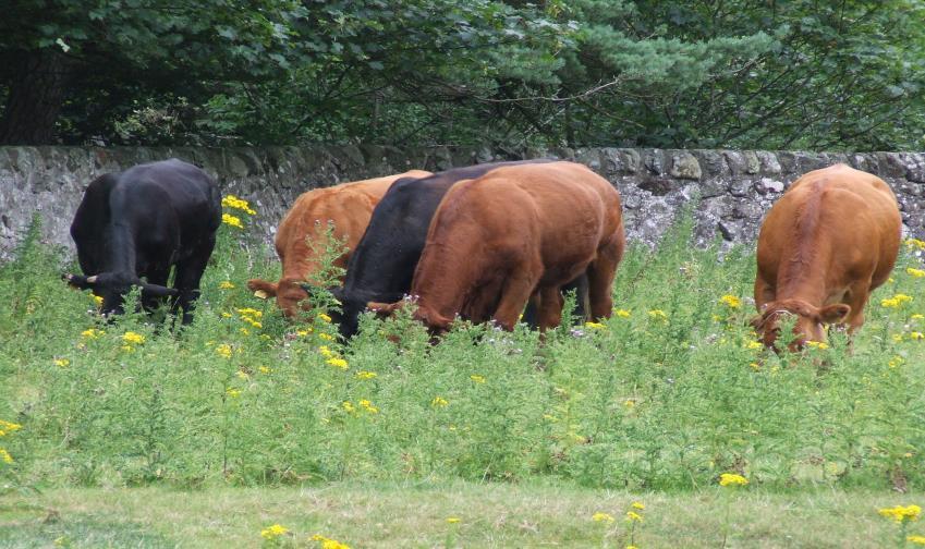
46 46