EVAPORATION FROM IRRIGATED AGRICULTURAL LAND IN CALIFORNIA

Transcription

1 Evaporation from Irrigation Agricultural Land in California EVAPORATION FROM IRRIGATED AGRICULTURAL LAND IN CALIFORNIA ITRC Report R January 2002 Funded by CALFED and CSU/ARI by C. M. Burt, A. Mutziger, D.J. Howes, and K.H. Solomon Irrigation Training and Research Center BioResource and Agricultural Engineering Dept. California Polytechnic State University (Cal Poly) San Luis Obispo, CA

2 Evaporation from Irrigation Agricultural Land in California EXECUTIVE SUMMARY The Research The stated intent of this research was to: 1. Consolidate existing information on evaporation through literature reviews and interviews. 2. Compute evaporation amounts for representative conditions in California and use those amounts to extrapolate information for the complete irrigated agricultural area of California. This research was to address the question of the approximate magnitude of evaporation - a key piece of knowledge when defining the level of resources that should be committed to solving any problem. It did not include field work. The research was funded through two different contracts: 1. CALFED 2. The Agricultural Research Initiative of the California State University (CSU/ARI). All work was conducted at the Irrigation Training and Research Center (ITRC) on the California Polytechnic State University (Cal Poly), San Luis Obispo campus. The research team gratefully acknowledges review comments and assistance during the process from a variety of sources, but in particular from Dr. Richard Allen of Univ. of Idaho and Dr. Terry Howell of USDA/ARS in Bushland, TX. Literature Review and Interviews An extensive literature review was made and is summarized in Chapter 3 of this report. A more detailed discussion of the literature is found in Appendix A. The following sections summarize the major points from the review. CALFED/ARI Evaporation Study i Irrigation Training and Research Center

3 Types of evaporation Evaporation from Irrigation Agricultural Land in California Three forms of evaporation loss were identified: 1. Soil evaporation a. Bare soil b. Soil under a crop canopy 2. Wet foliage evaporation 3. Spray loss from sprinklers (loss between the sprinkler and the plant or soil). Bare soil evaporation This form of evaporation represents the majority of annual evaporation. It is particularly important for precipitation and pre-irrigations when a crop is not growing in a field. Bare soil evaporation may extend much deeper than the 5-10 cm limit that is traditionally used in many irrigation scheduling models. The FAO-56 procedure that uses a 2-stage or 3-stage soil drying models appears to describe bare soil evaporation within ±15%. The effect of stubble and mulch on soil evaporation The usage of stubble, soil mulches, and no-till practices can provide a substantial reduction (11 84%) in shortterm evaporation when no crop is in the field. Long-term reductions are perhaps half of these amounts. Wet foliage evaporation Wet foliage evaporation is highly variable, ranging from a few percentage points to greater than 50% of the applied irrigation water. Small and frequent irrigations -- which can occur with high-speed linear moves or center pivots -- on a dense crop canopy, in very dry and hot conditions, produce the highest values. The increase in evaporation is partly offset by a decrease in transpiration, although the total ET with a wet canopy is higher (by as much as 60-70% in extreme cases) than for dry foliage in an unstressed condition. One must distinguish between evaporation as a percentage of the applied irrigation water, as a temporary (but short-term) increase in ET rate, or as a long-term increase in ET rate. Spray loss from sprinklers This aspect of evaporation has the most associated literature, and within the literature one finds the widest range of reported values (0.4 45%) of losses. Good recent research indicates that spray droplet evaporation losses are in the magnitude of 1 4% for typical sprinkler systems. The percentage can be higher for small nozzle sprinklers on wide spacings with high pressures. A single sprinkler operating by itself will have a higher spray loss because the surrounding air is less humid than if adjacent sprinklers were operating. Part of the differences in reported values appears to come from errors in measurement or from unusual testing conditions. CALFED/ARI Evaporation Study ii Irrigation Training and Research Center

4 Evaporation from Irrigation Agricultural Land in California Evaporation Modeling Methodology The FAO Irrigation and Drainage Paper No. 56 (Allen et al., 1998) defines a procedure for estimating crop evapotranspiration (ET field ). This procedure, with some modifications, allowed ITRC to compute year-long daily water balances using reference ETo and crop coefficients that account for the impacts of plant stress and wet soil and plant surfaces. Transpiration (T) and evaporation (E) components of ET were separated for both rainfall and irrigation. ITRC computed daily soil root zone and plant canopy water balances for 3 years on the major crop rotation patterns in agricultural areas of California. The daily water balance computations required knowledge of common irrigation schedules, the type and distribution of the various irrigation methods, planting dates, harvest dates, normal year rainfall patterns, etc. The computation procedure had the following variables: 1. Irrigated agricultural areas separated by 13 ETo Zones (Figure 1) as established by the California Department of Water Resources (DWR). Daily ETo data were obtained from the California Irrigation Management Information Systems (CIMIS) network. Detailed quality control checks of solar radiation and relative humidity were conducted on a representative sample of the station data. Some areas of California were excluded because of their low numbers of irrigated acreage, including the Northern California Coast, east of the Sierra Nevada and Cascade mountains, north of Redding, and parts of the desert in San Bernardino County. 2. Four typical soil types for each ETo Zone. Digitized soil survey data were obtained and were processed in ArcView GIS, along with crop data. 3. All major crops for each area. Digitized crop acreages for all ETo Zones were obtained through California DWR land use surveys. 4. Three successive years (1997, 1998, 1999) representing normal, wet, and dry years, respectively. 5. Various irrigation methods (drip/micro, sprinkler, and surface; with various subdivisions of each category). The acreages of various irrigation methods used on different crops and soils, by ETo Zone, were obtained from a variety of sources. These included irrigation district surveys, California DWR records as reported by the 1998 annual irrigation survey in the Irrigation Journal, and ITRC experience. Table 1 shows the estimated California irrigated acreage by crop and irrigation methods that were used in this evaluation. Crop planting and harvest dates were obtained from farmer interviews and published data available from the various local county extension publications of the University of California, Agricultural Commissioners, and irrigation districts in each Zone. Typical farmer irrigation practices were known from interviews with farmers and from the expertise of ITRC staff. CALFED/ARI Evaporation Study iii Irrigation Training and Research Center

5 Evaporation from Irrigation Agricultural Land in California Figure 1. DWR ETo zones. This study used zones 1-4,6,8-16, and 18. CALFED/ARI Evaporation Study iv Irrigation Training and Research Center

6 Evaporation from Irrigation Agricultural Land in California Table 1. Crop acreage by irrigation method in California. Crop All Furrow All Border Strip and Basin Combination Sprinkler/Furrow All Sprinkler All Drip/Micro Total Acreage Apple, Pear, Cherry, Plum and Prune 17,821 56, ,930 85, ,910 Peach, Nectarine and Apricots 12,537 38, ,367 55, ,085 Almonds 0 211, , , ,909 Walnuts 17,858 62, ,192 88, ,879 Pistachio 9,687 21, ,714 35,123 80,603 Misc. Decidous 4,698 13, ,858 21,631 47,495 Grain and Grain Hay 0 681, , ,284 Rice 0 379, ,989 Cotton 714, , ,428 40,403 1,122,140 Safflower and Sunflower 0 173, , ,795 Corn and Grain Sorghum 381, , , ,574 Beans 61, ,215 42,615 13, ,860 Misc. field crops 103, , ,687 27, ,313 Alfalfa Hay and Clover 37, , , ,312 Pasture and Misc. Grasses 0 357, , ,586 Small Vegetables 310, , ,057 86, ,337 Tomatoes and Peppers 151, , ,432 36, ,454 Potatoes, Sugar beets, Turnip ect. 59, ,865 61,071 15, ,621 Melons, Squash, and Cucumbers 57, ,567 55,200 14, ,451 Onions and Garlic 29, ,834 36,064 8,487 84,872 Strawberries , ,317 55,528 Flowers, Nursery and Christmas Tree 1,858 1, ,441 37,157 Citrus (no ground cover) 14,048 11, , , ,961 Avocado 2,756 2, ,616 55,129 Misc Subtropical 3,073 2, ,316 61,462 Unknown Grapes 202, , , ,469 Idle 186, ,829 Total 2,380,226 2,656, ,778 1,970,056 1,811,622 9,313,004 Results and Recommendations All results here are reported for calendar years, not for crop growing seasons. Therefore, crop ET might also be called annual field ET. Our values of annual field ET are higher than most published values, because those typically only include growing season ET. Table 2 shows that although the annual field ET for irrigated fields stays almost the same from year to year, the components of ET change dramatically especially the precipitation evaporation component. It also shows that although the effective precipitation ranges from 29% to 59% each year, the percentage of irrigation water that evaporates stays about the same (11%). Table 3 shows the evaporation information by crop, for typical soils and irrigation methods within each ETo zone. CALFED/ARI Evaporation Study v Irrigation Training and Research Center

7 Evaporation from Irrigation Agricultural Land in California Table 2. Annual results of the evaporation study. Typical, wet and dry refer to the amount of precipitation between January and April of that year (typical) 1998 (wet) 1999 (dry) E ppt - E from Precipitation (AF) 3,912,000 6,226,000 3,989,000 E irr - E from Irrigation (AF) 2,301,000 1,794,000 2,295,000 T ppt - T from Precipitation (AF) 518,000 2,708, ,000 T irr T from Irrigation (AF) 19,029,000 14,219,000 18,219,000 Total ET field (AF) 25,760,000 24,947,000 24,944,000 Total Precipitation (AF) 10,294,700 31,130,000 7,526,400 Total ET irr (AF) 21,330,000 16,014,000 20,514,000 % of Precipitation that Evaporates 38% 20% 53% % of Precipitation used for ET ppt 43% 29% 59% E irr, as a % of ET irr 11% 11% 11% CALFED/ARI Evaporation Study vi Irrigation Training and Research Center

8 Evaporation from Irrigation Agricultural Land in California Table average annual volumes of evaporation. The volumes assume existing irrigation methods. Average of Total Evap Eirr Eppt Crop Acre-ft Acre-ft Acre-ft Apple, Pear, Cherry, Plum and Prune 76,000 18,600 57,400 Apple, Pear, Cherry etc w/cover crop 43,100 16,900 26,200 Immature Apple, Pear, Cherry etc 34,000 10,400 23,600 Peach, Nectarine and Apricots 91,300 25,100 66,200 Immature Peach, Nectarine and Apricots 22,800 7,700 15,100 Almonds 252,200 68, ,300 Almonds w/ cover crop 86,300 34,600 51,700 Immature Almonds 109,200 49,600 59,600 Walnuts 133,700 27, ,900 Immature Walnuts 36,300 10,900 25,400 Pistachio 42,200 9,800 32,400 Pistachio w/ cover crop 11,400 4,000 7,400 Immature Pistachio 14,300 4,900 9,400 Misc. Deciduous 32,900 8,400 24,500 Immature Misc. Deciduous 8,300 2,700 5,600 Grain and Grain Hay 391, , ,900 Rice 401, , ,300 Cotton 876, , ,700 Safflower and Sunflower 127,900 20, ,900 Corn and Grain Sorghum 483, , ,900 Beans 118,000 31,900 86,100 Misc. field crops 210,800 67, ,000 Alfalfa Hay and Clover 443, , ,400 Pasture and Misc. Grasses 421, , ,500 Small Vegetables (Double Crop) 738, , ,600 Tomatoes and Peppers 281,000 42, ,300 Potatoes, Sugar beets, Turnip ect. 74,400 19,400 55,000 Melons, Squash, and Cucumbers 124,400 33,500 90,900 Onions and Garlic 36,700 11,000 25,700 Strawberries 46,700 8,100 38,600 Flowers, Nursery and Christmas Tree 30,300 5,600 24,700 Citrus (no ground cover) 152,800 48, ,400 Immature Citrus 42,900 14,000 28,900 Avocado 42,400 8,100 34,300 Misc Subtropical 40,100 13,800 26,300 Grape Vines 387,200 71, ,800 Grape Vines w/ cover crop 134,400 34, ,200 Immature Grape Vines 106,400 21,400 85,000 Idle 127, ,800 Total 6,834,800 2,125,900 4,708,900 CALFED/ARI Evaporation Study vii Irrigation Training and Research Center

9 Evaporation from Irrigation Agricultural Land in California The statewide annual field ET for irrigated acreage is about the same regardless of irrigation method (Table 4). Although the values are sometimes incorrectly interchanged, Field ET is not to be confused with gross irrigation water applied, which includes irrigation water only, some of which may be destined to runoff and deep percolation as well as ET. Field ET includes more than just irrigation water, and isn t a measurement of how much water is applied to a system, but rather how much is used/lost by a system. There are always special cases, but these values are representative for the typical irrigation methods found in California. For small vegetables (lettuce, broccoli, etc.), there is a greater difference between methods (Table 5). Table 4. Annual field ET for cotton in the central San Joaquin Valley (ETo Zone 15). This is for a typical year, and values have been de-rated by 10% for bare spots and decreased vigor on parts of a typical field. Inches. Irrigation Method Irrig. Evap. Precip. Evap Transpiration Field ET Surface Sprinkler Drip/micro Table 5. Typical year annual field ET for small vegetables near Salinas (2 crops/yr assumed). This is for a typical year, and values have been de-rated by 10% for bare spots and decreased vigor on parts of a typical field. The drip irrigation is assumed to use sprinklers for germination, leaching, and early season irrigations, and surface drip irrigation for the remainder of the growing season the typical practice in the area. Inches. Irrigation Method Irrig. Evap. Precip. Evap Transpiration Field ET Surface Sprinkler Drip/micro For most of the report, drip and microirrigation (drip/micro) was assumed to have a 40% average wetted soil surface. However, separate crop models were run for pistachios and almonds in the San Joaquin Valley to assess the sensitivity of evaporation and ET to percent wetted area. Figure 2 shows the results of this comparison. Approximately half of the almond acreage uses microsprayers, which have a wetted fraction of Evaporation of irrigation water ranges from 2 10% wetted area to 10 80% wetted area. Overall, the study estimated that ETc on drip/micro is 6 10% higher under drip/micro than under surface or sprinkler irrigation. This does not say anything about the impact on yield and energy or the suitability of one method or another for the topography and size of field. CALFED/ARI Evaporation Study viii Irrigation Training and Research Center

10 Evaporation from Irrigation Agricultural Land in California E and ET, mm Percent Wetted Fraction of the Soil Annual ETc with Stress Annual Evap. of Irrig. Water with Stress Annual ETc w/o Stress Annual Evap. of Irrig. Water w/o Stress Figure 2. Crop ET and E as a fraction of wetted area. Stressed and non-stressed almond trees irrigated with drip or microsprayers in ETo Zone 15 (San Joaquin Valley). No adjustment for vigor or bare spots. When the quantities involved in a calculated result are not known with certainty, the result calculated is also subject to some uncertainty. The uncertainty of the result is determined by the uncertainty of the quantities involved and by the manner in which these quantities are combined in the calculation process. These uncertainties can be expressed as confidence intervals (CI), and their determination is the subject of confidence interval analysis. Chapter 6 and Appendix L provide a detailed explanation of how the CI was computed for the final estimate of evaporation. Consideration of the results suggests that our ability to predict evaporation from the current data and procedures is no worse than our ability to predict ET, and supports the contention that CI{Statewide Evaporation from Irrigated Fields} = ± 17% as illustrated in Figure 3. CALFED/ARI Evaporation Study ix Irrigation Training and Research Center

11 Evaporation from Irrigation Agricultural Land in California Relative Likelihood of Estimate State-Wide Evap from Irrig Fields (typ yr) Most likely estimate = 5.9 million ac-f t 95% Conf idence Limits: Lower = 4.9 million ac-f t Upper = 6.9 million ac-f t Estimated Annual Evaporation (million acre-fee Figure 3. Confidence Interval for Statewide Evaporation from Irrigated Fields. Recommendations for further research (Chapter 7) include: 1. An economic analysis of the conservation potential should be developed. For example, the total average annual evaporation from irrigation is estimated to be approximately 2.7. An investment in Subsurface Drip Irrigation (SDI), which might cost $1,000/acre, might save half of this water. The estimated cost/af conserved should be compared with other available conservation options. 2. Because the majority of annual evaporation is from precipitation (4.7 million AF/year, or 69% of the total evaporation), research on conserving precipitation water through mulches and tillage practices should be expanded. 3. What is not known is how evaporation reduction within a field impacts the surrounding region. For example, an increase in evaporation in one field may increase the relative humidity of the air, and therefore reduce the ET in downwind fields. Further research could approach this problem both with localized remote sensing and also theoretically based on the apparent local rise in relative humidity. 4. The issue may not be so much one of reducing evaporation and transpiration, as it is one of increasing crop yield per unit of ET. Therefore, research, demonstration projects, and information dissemination on related topics such as optimizing fertigation practices is of high priority. 5. State and Federal programs that either report ET or require the reporting of ET should be consistent on the following: a. The crop ET for water balances should be de-rated (by 10% as a rough starting approximation) to account for bare spots and lack of vigor throughout fields. This is in contrast to ET values to be used for irrigation scheduling. Both sets of values are provided on ITRC s web page CALFED/ARI Evaporation Study x Irrigation Training and Research Center

12 Evaporation from Irrigation Agricultural Land in California b. ET values for irrigation district water balances should be for a year, not just for a crop season. 6. The California DWR CIMIS program should initiate a new type of quality control program which performs a quality control check on the historical solar radiation (Rs) and relative humidity values for each weather station. Corrections should be made to erroneous data. CALFED/ARI Evaporation Study xi Irrigation Training and Research Center

13 Evaporation from Irrigation Agricultural Land in California TABLE OF CONTENTS Executive Summary... i The Research... i Literature Review and Interviews... i Types of evaporation... ii Evaporation Modeling Methodology... iii Results and Recommendations... v Table of Contents... xii List of Figures... xv List of Tables...xviii List of Appendices... xxi 1 Introduction Background Methodology FAO Drainage and Irrigation Publication No. 56 Procedure for Calculating Evapotranspiration Why FAO-56? FAO 56 Modifications Study Regions Average Weather Station Selection of the Years for Detailed Water Balance Basic Data for Study Soils and Irrigation Systems Importance of Information Sources of Information Procedures for Estimating Acreage Total Crop Acreage Weather Data Rainfall Variability Review and Interpretation of Evaporation Research Background What Falls under "Evaporation" Evaporation Equations Soil Evaporation FAO-56 Method and Modifications CALFED/ARI Evaporation Study xii Irrigation Training and Research Center

14 Evaporation from Irrigation Agricultural Land in California Bare Soil Evaporation Without Stubble or Mulch Effect of Stubble and Mulch on Soil Evaporation in the Field Soil Evaporation with Drip Irrigation Evaporation from Plant Surfaces Wet Foliage Evaporation Observations and Discussion Other E and T Partitioning Leaf Water Storage and Potential Applications for Coupled Energy & Water Balance Methods Sprinkler Droplet (in air) Evaporation Loss Measured and Simulated Spray Loss Rain Gauge Errors Water Source Temperature Effect on Spray Loss Impact of Wet Bulb Temperature on Sprinkler Evaporation Impact of Droplet Flight Time and Spray Drift on Sprinkler Evaporation Impact of Droplet Size and Nozzle Height on Sprinkler Evaporation References Possible Information Sources on Rain Gauge Errors Other Rainfall-related Resources Daily Water Balance FAO 56 Daily Water Balance Model Input Parameters to FAO Basal Crop Coefficients (Kcb) Imposed Crop Stress Subdivision of Soil Evaporation into Precipitation and Irrigation Water Origin Evaporation from Wet Plant Surface with Sprinkler Irrigation Gross Adjustments Evaporation Sensitivity to Variation in Wetted and Exposed Fractions of the Soil Results and Discussion Total Evaporation and Transpiration Evaporation of Precipitation Comparison of Irrigation Methods Variations within the Drip/Micro Method Comparison of Irrigation Methods Assuming Different Types of Drip/Micro Statewide partitioning of ETc components by irrigation method Annual Crop Coefficients (ETc/ETo) Confidence Intervals CI Analysis - Statewide Volume of Evaporation from Irrigated Fields CI Perspective Confidence Interval Analysis CALFED/ARI Evaporation Study xiii Irrigation Training and Research Center

15 Evaporation from Irrigation Agricultural Land in California 6.2 Confidence Intervals for Key Parameters in the Estimation of Statewide Evaporation Volume from Irrigated Fields ETo for Each Station (Station ETo) ETo for Each Zone (ETo z ) Irrigated Area by Crop and Zone (Area z,c ) Portion of Crop Area Irrigated by Each System Type (P z,c,i ) Field-Crop System Coefficients The Evaporation Fraction of Evapotranspiration from the Field-Crop System (Fe) Summary of Confidence Interval Estimates Results of Confidence Interval Analysis Zone Evaporation and CI's State Evaporation and Confidence Interval Discussion References Recommendations Information Dissemination References Weather Data Bibliography Related to Precipitation Measurements Misc Rainfall variability CALFED/ARI Evaporation Study xiv Irrigation Training and Research Center

16 Evaporation from Irrigation Agricultural Land in California LIST OF FIGURES Figure 1 Figure 2 Figure 3 DWR ETo zones. This study used zones 1-4,6,8-16, and iv Crop ET and E as a fraction of wetted area.... ix Confidence Interval for Statewide Evaporation from Irrigated Fields.... x Figure 1-1 Cumulative grass reference evapotranspiration (ETo) used in the selection of years for the detailed water balance Figure 1-2 Annual Precipitation used in the selection of years for the detailed water balance Figure 2-1 California Crop Acreage by Soil Category Figure 2-2 Total Acreage throughout California by Irrigation Type Figure 3-1 Cumulative evaporation depth (De) versus the FAO - 56 soil evaporation reduction coefficient (Kr) (Allen et al, 1998) Figure 3-2 Ratio of daily bare soil evaporation (Ed) to daily potential soil evaporation (Epd) Figure 3-3 Comparison of loam soil Kr relationships Figure 3-4 Comparison of silty clay loam soil Kr relationships Figure 3-5 Comparison of clay soil Kr relationships Figure 3-6 Comparison of bare soil E/ETo ratios Figure 3-7 Comparison of bare soil cumulative evaporation Figure 3-8 Lysimeter with Houston black clay soil used by Ritchie and Adams (1974) Figure 3-9 Crop evapotranspiration and evaporation as the fraction of wetted area Figure 3-10 The Cupid simulated partitioning of ET during an 8-day measurement period Figure 3-11 Diurnal water budget for Julian day 202 with no irrigation or rainfall Figure 3-12 Diurnal water budget for day 202 assuming 12 mm of rain late on day Figure 3-13 Diurnal water budget for day 202 assuming 36.1 mm of irrigation water was applied Figure 3-14 Cumulative water loss budget for 3 simulated water application cases Figure 3-15 DPEVAP model prediction of droplet flight time as related to droplet size and wind speed Figure 3-16 Rate of droplet volume loss (% s -1 ) as related to the initial droplet diameter for hot dry air CALFED/ARI Evaporation Study xv Irrigation Training and Research Center

17 Evaporation from Irrigation Agricultural Land in California Figure 3-17 Rate of droplet volume loss (% s -1 ) as related to the initial droplet diameter for moderate temperature Figure 3-18 DPEVAP model prediction of droplet evaporation as related to droplet diameter and nozzle height Figure 4-1 Simple two dimensional root zone water balance Figure 4-2 Crop water stress coefficient, Ks, related to management allowable depletion of total available water to the crop Figure 5-1 Department of Water Resources Grass Reference Evapotranspiration Zone Map Figure 5-2 Three year average annual evaporation volume (acre-ft) by crop for California s irrigated agricultural acreage Figure 5-3 Percentage of total evaporation partitioned into that from irrigation water and that from precipitation Figure average percent of the total precipitation that evaporates, correlated with annual precipitation amounts averaged for all zones Figure 5-5 Total depth of crop ET for Cotton in ETo Zone Figure 5-6 Components of Small Vegetable ET by irrigation method near Salinas Figure 5-7 Crop evapotranspiration and evaporation as the fraction of wetted area. Stressed and non-stressed almond trees irrigated with drip or microsprayers in ETo Zone Figure 5-8 Crop evapotranspiration and evaporation as the fraction of wetted area. Stressed and non-stressed pistachio trees irrigated with drip or microsprayers in ETo Zone Figure 5-9 Comparison of total annual ETc components for all crops by irrigation method Figure 5-10 Year-to-year crop coefficient (Kc) comparison for surface irrigated almonds in Zone Figure 5-11 Crop coefficient year-to-year comparison for surface irrigated cotton in Zone Figure 5-12 Three year average crop coefficient comparison by soil type Figure 5-13 Crop coefficient comparison for surface irrigated cotton in Zone 15 by soil type Figure 5-14 Comparing crop coefficients for irrigation methods on almonds in Zone Figure 5-15 Comparing crop coefficients for irrigation methods on cotton in Zone Figure 6-1 CI analyses are based on model outputs rather than on the numerous and detailed calculations within the model Figure 6-2 Most crops are grown in multiple zones Figure 6-3 Confidence interval estimate for Zone 14 ETo CALFED/ARI Evaporation Study xvi Irrigation Training and Research Center

18 Evaporation from Irrigation Agricultural Land in California Figure 6-4 The uncertainties in P su, P sp and P dm are conditioned by the fact that the three proportions must add to one Figure 6-5 Confidence Interval for Statewide Evaporation from Irrigated Fields Figure 6-6 Contributions of the uncertainties in key parameters to the confidence interval for the statewide estimate for evaporation from irrigated fields CALFED/ARI Evaporation Study xvii Irrigation Training and Research Center

19 Evaporation from Irrigation Agricultural Land in California LIST OF TABLES Table 1 Table 2 Table 3 Table 4 Table 5 Crop acreage by irrigation method in California.... v Annual results of the evaporation study.... vi average annual volumes of evaporation.... vii Annual field ET for cotton in the central San Joaquin Valley (ETo Zone 15)....viii Typical year annual field ET for small vegetables near Salinas (2 crops/yr assumed)...viii Table 1-1 Study regions for detailed analysis Table 1-2 Other regions in the study Table 2-1 Crop and Soil Acreage Summary for California Table 2-2 Crop Acreage by Irrigation Method Table 2-3 CIMIS Stations used for the evaporation study Table 3-1 Table 3-2 Table 3-3 Range of FAO - 56 parameters for defining the evaporation reduction coefficient (Kr) relationship for loam, silty clay loam, and clay soils (Allen et al, 1998) FAO - 56 parameters selected by the authors to determine the average evaporation reduction coefficient (Kr) for loam, silty clay loam, and clay soils Comparison of FAO - 56 simulated evaporation against various field measurements of evaporation Table 3-4 Bare soil evaporation with different soils and densities (Prihar et al., 1996) Table 3-5 Table 3-6 Relative evaporation for a crack in Houston black clay with and without the contribution of evaporation from the soil adjacent to the crack (Ritchie and Adams, 1974) Soil evaporation as a function of soil depth for Weld silt loam (Shawcroft and Gardner, 1983) Table 3-7 Specifications of micro-lysimeters used in studies evaluated in this paper Table 3-8 Table 3-9 Effect of surface mulch rates on one day of evaporation from bare loamy sand soil (Hares and Novak, 1992b) month soil evaporation reduction using no-till w/ standing stubble for bare Fargo- Ryan silty clay soil in dryland conditions (Brun et al., 1986) Table day soil evaporation reduction using no-till and planting in standing stubble for Olton sandy clay loam with limited irrigation (Lascano et al., 1994) CALFED/ARI Evaporation Study xviii Irrigation Training and Research Center

20 Evaporation from Irrigation Agricultural Land in California Table day soil evaporation reduction using a surface mulch on a bare Cozad silt loam soil for three irrigation conditions (Todd et al., 1991) Table day soil evaporation reduction using no-till and planting in standing stubble with the addition of surface mulch to a Cozad silt loam soil for three irrigation conditions (Todd et al., 1991) Table 3-13 Comparison of cumulative corn crop water budget from Cupid with field measurements Table 3-14 Summary of hourly environmental data during an 8-day measurement period Table 3-15 Example of detailed crop canopy and soil surface energy balance components Table 3-16 Estimates of the percentage of time during a growing season (with 100 days of canopy) that foliage evaporation occurs for sprinkler irrigation systems Table day soil evaporation and transpiration reduction using no-till and planting in standing stubble for Olton sandy clay loam with limited irrigation (Lascano et al., 1994) Table 3-18 Impact of water temperature on sprinkler spray loss as measured in the field with electrical conductivity change (Mclean et al., 1994) Table 3-19 DPEVAP simulated impact of water temperature on sprinkler spray loss for hot dry conditions (Thompson et al., 1993a) Table 4-1 Table 4-2 MAD threshold and MAD used for irrigation scheduling for Zone 15 with surface irrigation Evaporation of irrigation water sensitivity to the wetted and exposed fraction of the soil Table 5-1 Complete annual results of the evaporation study Table 5-2 Results for a typical precipitation year (1997) annual crop evapotranspiration Table 5-3 Results for a typical precipitation year (1997) composite annual transpiration Table 5-4 Results for a typical precipitation year (1997) annual evaporation of irrigation water Table 5-5 Results for a typical precipitation year (1997) annual evaporation of precipitation water Table average annual volumes of evaporation Table 5-7 Average annual evapotranspiration for all crops by zone Table 5-8 Average annual total crop evapotranspiration and its components by zone Table 5-9 Percentage of total precipitation that is lost to evaporation Table 5-10 Annual ETc for cotton in ETo Zone Table 5-11 Components of Small Vegetable ETc by irrigation method CALFED/ARI Evaporation Study xix Irrigation Training and Research Center

21 Evaporation from Irrigation Agricultural Land in California Table 5-12 Crop evapotranspiration and evaporation as the fraction of wetted area. Stressed and non-stressed almond trees irrigated with drip or microsprayers in ETo Zone Table 5-13 Crop evapotranspiration and evaporation as the fraction of wetted area. Stressed and non-stressed pistachio trees irrigated with drip or microsprayers in ETo Zone Table 5-14 Irrigation method comparison for mature almonds without cover crops for Zone Table 5-15 Irrigation method comparison for mature pistachios without cover crops for Zone Table 5-16 Composite average annual calculated crop coefficients for all crops throughout California with existing irrigation methods and scheduling Table 6-1 Estimated values for ε by Crop and Zone Table 6-2 Table 6-3 Difference in estimates of grass reference evapotranspiration (ETo) based on corrected and uncorrected weather data CI{Zone Irrigated Area}, CI{Statewide Crop Area} and CI{Statewide Irrigated Area} as Influenced by CI{Individual Crop/Zone Area Estimates} Table 6-4 Confidence intervals for various areas, based on CI{Crop/Zone Area} = ± 10% Table 6-5 Confidence intervals for estimates of irrigated area by crop category and zone Table 6-6 Comparisons of calculated and measured evaporation from bare soil Table 6-7 Summary of CI estimates for key parameters Table 6-8 Evaporation estimates and confidence intervals for each zone Table 6-9 Contributions to the overall CI of individual parameter CI's Table 6-10 Comparison of CI's for Model Parameters and Zone ET's CALFED/ARI Evaporation Study xx Irrigation Training and Research Center

22 Evaporation from Irrigation Agricultural Land in California LIST OF APPENDICES Appendix A Literature Review Appendix B FAO-56 Crop Evapotranspiration Model Appendix C Evaluating the Quality of Uncorrected CIMIS ETo Data Appendix D Crop Acreage Appendix E Comparison of Measured and FAO Modeled Bare Soil Evaporation Appendix F Crop Parameters Appendix G Bare Spots and Evaporation from Field Edges Appendix H Reality Check of ET Values Appendix I Results by Irrigation Systems Appendix J ETc and Evaporation Final Results Appendix K Drip/Microspray Evapotranspiration Evaluation Appendix L Introduction to Confidence Levels CALFED/ARI Evaporation Study xxi Irrigation Training and Research Center

23 Evaporation from Irrigation Agricultural Land in California 1 INTRODUCTION 1.1 Background California's economic and environmental well-being is closely linked to the state's water management. Water conveyance and utilization consume large amounts of energy in the state. Future scenarios of how much water will be pumped from the groundwater and from the Delta, as well as future energy needs, all require good estimates of water balances. However, some of the fundamental data that is used for planning contains large uncertainties. All California irrigation districts that receive either federal or state water are now required to prepare Water Conservation Plans. For the first time in the history of most districts, they are developing an elementary water balance. The term "elementary" should be emphasized, because there are significant weaknesses in our knowledge of subsurface flows and some components of Evapotranspiration (ET). Irrigation districts generally use published "typical" values of ET for their water balance computations. Basic weaknesses with published values for ET include: 1. The values are published as "ET" rather than Evaporation and Transpiration components. 2. Most values only include estimates of ET during the crop growing season, and ignore ET during the rest of the year and on fallow ground. 3. There is no separation of the evaporation contribution of irrigation vs. rainfall. 4. Published ET values do not account for differences in irrigation and soil management. Therefore, one cannot estimate the impact of various management practices on the volumes of evaporation that might occur under difference scenarios. CALFED/ARI Evaporation Study 1 Irrigation Training and Research Center

24 Evaporation from Irrigation Agricultural Land in California While it is clearly understood that evaporation losses occur, it is considerably less certain what the values are. Furthermore, the assumption in the irrigation and state planning sectors has typically been that the evaporation values are quite small. This assumption was tested in the research that is described in this report. At the beginning of this research, we had a general understanding that evaporation on irrigated agricultural lands may represent somewhere between 5% and 25% of the total ET - hardly a precise value. Of course, there is the additional question: Even if we know what the magnitude of the evaporation is, can we do anything about it? That question can be answered in part by understanding when and how the evaporation occurs, as well as by knowing its magnitude. If the evaporation is much larger than earlier believed, that knowledge may justify the application of various reduction measures that were previously discarded as being overly expensive. On the other hand, if evaporation is much less than some believe, it may indicate that there is very little savings possible and therefore investments to reduce evaporation (such as investing in subsurface drip irrigation for the intended purpose of reducing water consumption) would be unwise. But without the knowledge, we have no basis for action in either direction. A frequently heard theory is that drip irrigation may decrease crop ET - or at least decrease the evaporation component of ET. Some limited studies have been done to document such ET. However, one must recognize that there are many forms of "drip". The majority of systems in California are placed on the soil surface, and there are tremendous differences among soil coverage, plant shading, and wetting patterns of various drip and microspray and microsprinkler systems. Even if one focuses on buried drip (subsurface drip irrigation, or SDI), there are huge differences. Some utilize sprinkler or surface irrigation at some times of the year (with the accompanying evaporation). In summary, there are 2 primary questions: (i) is evaporation significant, and (ii) is it worthwhile to invest in technologies or practices that could conserve some of this evaporation. The research reported here addresses the first question, and provides a partial answer to the second. 1.2 Methodology This research reduces the uncertainty in the estimate of evaporation from irrigated agricultural fields in California. Although it does not include evaporation from canals or riparian areas, it provides a best estimate of irrigation water and rainwater field evaporation. One cannot compute evaporation, however, without knowing how frequently the soil is wet and how quickly the soil surface will dry due to competing transpiration. Therefore, this study computed both evaporation and transpiration through the following procedure: CALFED/ARI Evaporation Study 2 Irrigation Training and Research Center

25 Evaporation from Irrigation Agricultural Land in California 1. The acreage of various crops in California, as well as the locations, growing seasons, and methods of irrigation have been estimated based on data from Water Conservation Plans submitted by irrigation districts, DWR crop surveys, and County Agricultural Commissioners Reports. 2. Farmers were interviewed to verify planting, harvesting, and irrigation dates. Rainfall events and ETo data were obtained from CIMIS weather stations. Quality control checks on incoming solar radiation and relative humidity values were done to obtain a confidence interval for the ETo data. 3. Research reports on evaporation were reviewed. These include research reports on sprinkler drift/spray losses, as well as wet soil evaporation studies. 4. A review meeting was held with key researchers who have been involved with this subject. 5. The revised FAO procedure for estimating crop evapotranspiration (Allen et al. 1999) was used to compute daily soil root zone water balances for 3 years on the major crop rotation patterns in agricultural areas of California. The daily water balance computations required knowledge of common irrigation schedules, the type of irrigation method, planting dates, harvest dates, normal year rainfall patterns, etc. Daily values of evaporation and transpiration were computed, and the evaporation values were further subdivided into (i) rainfall and (ii) irrigation water origins. ITRC has a working model in place for this type of computation. The FAO procedure defines a 2 or 3 stage soil surface drying function, depending upon the soil type. The computation procedure has the following variables: - Agricultural areas separated by ETo Zones - 4 typical soil types for each area - All major crops for each area - 3 successive years (1997, 1998, 1999) 6. Confidence intervals have been assigned to the components and final values. This report will highlight where the weak points are in our knowledge, and the relative impact of each weak point on the final estimates. This study is limited to estimated evaporation on irrigated agricultural land, and does not include evaporation estimates from other sources such as canals, rivers, streets, watersheds, and dryland farming. The study did not include irrigated acreages north of Redding, on the northern coast, east of the Sacramento and San Joaquin Valleys, or desert areas in San Bernadino County. CALFED/ARI Evaporation Study 3 Irrigation Training and Research Center

26 Evaporation from Irrigation Agricultural Land in California 1.3 FAO Drainage and Irrigation Publication No. 56 Procedure for Calculating Evapotranspiration Commercial irrigation schedulers typically begin their computation with published regional crop coefficients. These coefficients, when multiplied by reference crop evapotranspiration, are used to calculate crop evapotranspiration. These regional crop coefficients are based on a certain reference crop, soil type, and irrigation management practice. In conventional agriculture irrigation scheduling, crop coefficients can be modified as needed during the growing season, because there is constant feedback based on field observations of crop and soil conditions. Over the past 35 years, relatively good techniques have been developed to predict crop coefficients that reflect changes in irrigation management, soil moisture stress, and other conditions. Some of the techniques have been refined using weighing lysimeters; others have liberally used field observations of soil moisture content and changes. The preferred method of determining a crop coefficient (Kc) is to split the computation into 2 components. One is the transpiration component; the second is the evaporation component. This is called the dual crop coefficient methodology. A third component, lack of soil moisture and its impact on transpiration reduction, must also be included. The basal crop coefficient (Kcb) is the fraction of reference evapotranspiration that will equal the potential transpiration of a certain plant plus a small component of evaporation from a dry soil surface. The Kcb value will vary with the growth stage of the plant; for an annual crop it typically has a value of 0.15 near planting, and reaches a maximum value of or so at full cover. The product of (Kcb ETo) equals the crop ET under a well-watered condition with no stress and a dry soil surface. These conditions are very rare in a field application. The Kcb has no irrigation management component, or soil type component (it assumes perfect irrigation scheduling and a small water vapor evaporation component from the subsoil). Therefore, in concept it is transferable to anywhere in the world with little adjustment (the adjustments needed are for monthly average minimum relative humidity and wind speed (Allen et al, 1998)). CALFED/ARI Evaporation Study 4 Irrigation Training and Research Center

27 Evaporation from Irrigation Agricultural Land in California For actual estimates of crop ET, the basal crop coefficient is adjusted based on the amount of water stress that occurs, and an additional computation accounts for wet soil surface evaporation. Most crops undergo some amount of water stress throughout the growing period. Water stress occurs at a certain moisture depletion level. This level varies depending on the crop and its resistance to water stress. The dual crop coefficient method uses a crop stress coefficient (Ks) as a multiplier to reduce the potential transpiration because of the plant response to water stress. Therefore, the actual transpiration is [Ks*Kcb]*ETo, minus a small amount of evaporation inherent in Kcb. For most California crop ET estimates, if standard Kcb values were used (without factoring in Ks), the crop ET would frequently exceed the total amount of water applied via rain and irrigation. The evaporation component of the crop coefficient is the evaporation coefficient (Ke). It is calculated based on soil type and the evaporable water in the upper region of the soil. The evaporable water in this upper region is determined using a soil water balance. The overall equation using the dual crop coefficient to calculate ETc is: ETc = [Ks*Kcb + Ke] * ETo For a more detailed look at the dual crop coefficient method see Appendix B and FAO Why FAO-56? It was felt that the FAO 56 procedure was the best physically based approach to estimate what evaporation was. Furthermore, the daily water balance program allows the user to estimate where the evaporation water originated (rain or irrigation water). The benefits of this model help in interpretation of results and recommendations for the future FAO 56 Modifications Several modifications to the FAO - 56 procedure were necessary for this study. They were: 1. Partitioning the evaporation into precipitation and irrigation origins. Evaporation on the day of a precipitation event, and the days following that event, was designated as evaporation from precipitation until the available precipitation water was used. 2. The initial basal crop coefficient (Kcb) represents evaporation. Initial Kcb values range from As a plant emerges or grows leaves, the evaporation portion of this Kcb declines. The partitioning procedure between evaporation and transpiration for the initial Kcb is described in section B-1.2 of Appendix B. 3. Evaporation from wet plant surfaces was computed 2 days for each sprinkler application. The evaporation for those 2 days was set as the difference in ETo between a stomatal resistance of 0 s/m and 70 s/m. 4. A 3 rd stage of evaporation was included, to account for evaporation from open cracks on cracking clay soils and reduced vapor diffusion on some silt loam soils. CALFED/ARI Evaporation Study 5 Irrigation Training and Research Center

28 Evaporation from Irrigation Agricultural Land in California 1.4 Study Regions The irrigated agricultural land in California was split into 13 zones based on the California Department of Water Resources (DWR) 18 ETo zones. A majority of the agricultural land is found in 13 of these 18 ETo zones. Five of these zones were selected for detailed analysis dealing with planting and harvest dates and irrigation application amounts. Analysis of crop acreage, major soil types, irrigation methods, crop evapotranspiration (ETc), and evaporation was done for all 13 zones. The 5 zones used for detailed analysis and their general locations can be seen in Table 1-1. These zones were selected due to their spatial distribution in California and their diversity of crops. Computations for each of the other 8 zones (Table 1-2) used crop information (i.e. planting and harvest dates) from one of these 5 zones based on geographical, climate, and cropping similarities. Table 1-1. Study regions for detailed analysis. Zone 6 Inland Salinas Valley down to San Luis Obispo county. Santa Ana Region of Southern California Zone 12 Eastern San Joaquin Valley from Tulare to San Joaquin Counties and parts of Glenn, Colusa and Sutter Counties in Northern California. Zone 14 Northern California Central Valley from Stanislaus to Tehama counties. Zone 15 Central and Southern San Joaquin Valley Zone 18 Imperial and Coachella Valleys Table 1-2. Other regions in the study. Zone 1 Extreme coastal region crops mainly grown in Monterey and Santa Barbara counties. Zone 3 Coastal valleys and plains. Zone 4 South coast Zone 8 North and inland from San Francisco Bay consisting of Solano, Lake and Napa Counties Zone 9 South coast marine to desert transition Zone 10 Central coast mountain range Zone 13 Northern Sierra Nevada s Zone 16 Westside of the central San Joaquin Valley Average Weather Station Weather data was collected from every CIMIS weather station in the 13 zones that had data available for The weather station data was averaged for each zone so that one complete set of weather data was available for each zone. This was considered an average weather station in each zone. This was done to buffer any data errors or weather parameter differences within each zone. CALFED/ARI Evaporation Study 6 Irrigation Training and Research Center

29 Evaporation from Irrigation Agricultural Land in California 1.5 Selection of the Years for Detailed Water Balance Irrigation amounts can vary from year to year, so this study used 3 different years of data to study evaporation amounts. Four spatially diverse CIMIS stations throughout California were used to help determine which years would be used for the study. From these CIMIS stations, June through September cumulative annual ETo and precipitation were analyzed for 15 years worth of data. The cumulative ETo for June through September showed little difference from year to year (Figure 1-1). It was decided that because the ETo values were so consistent from year-to-year, ETo differences could not be used to classify years. Instead, the annual precipitation was used as the basis for selecting which 3 years to study. Figure 1-2 shows that the three consecutive years of 1997, 1998, and 1999 give a good range of precipitation values. They represent a wide range: 1997 being a typical year, 1998 a very wet year, and 1999 a dry year. CALFED/ARI Evaporation Study 7 Irrigation Training and Research Center

30 Evaporation from Irrigation Agricultural Land in California Figure 1-1. Cumulative grass reference evapotranspiration (ETo) used in the selection of years for the detailed water balance. CALFED/ARI Evaporation Study 8 Irrigation Training and Research Center

31 Evaporation from Irrigation Agricultural Land in California Figure 1-2. Annual Precipitation used in the selection of years for the detailed water balance. CALFED/ARI Evaporation Study 9 Irrigation Training and Research Center

32 Evaporation from Irrigation Agricultural Land in California 2 BASIC DATA FOR STUDY Computations for evaporation required information regarding crop acreage, weather, irrigation methods, and soil types throughout California (with the exception of areas previously noted). Various sources for this information were used. Some of these sources include California Department of Water Resources, County Ag Commissioners, Natural Resource Conservation Service, CIMIS weather service, farmers, and irrigation and water districts throughout California. 2.1 Soils and Irrigation Systems Importance of Information An accurate prediction of evaporation requires accurate information on planting and harvest dates, irrigation methods and scheduling, crop type, and crop rotations within a region. Furthermore, there may be linkages between crops, soil, and irrigation methods used. All of these factors will effect a model's predication of crop evapotranspiration, total evaporation, and the partitioning of precipitation evaporation and irrigation water evaporation. This study used the sources of information described below Sources of Information California Department of Water Resources The California Department of Water Resources (DWR) carries out land use surveys throughout California. It generally conducts surveys by county or region. Surveys from about 1991 to 1998 have been digitized and can be used in a mapping computer program such as AutoCAD or ArcView GIS. This data has attributes for each field within a county or region, including crop types grown during the survey year, the number of crops grown on each field that year, the acreage for the field, its spatial reference and more. CALFED/ARI Evaporation Study 10 Irrigation Training and Research Center

33 Evaporation from Irrigation Agricultural Land in California The DWR surveys were the primary source of crop acreage data, although locally-developed data was used for Imperial Valley. The digitized data became very useful when digitized soils data was overlaid with the land use data and the attributes were combined (see Appendix D). For 90% of the study area, it was possible to obtain information that related crop type to soil type County Ag Commissioner Crop Reports County Agricultural Commissioner Crop Reports for California Counties were useful as an acreage check against DWR surveys and for the remaining 10% of the crop acreage that was not obtained from the DWR (see Appendix D) National Resource Conservation Service Soil Survey Division Digitized soil survey data was obtained from the SSURGO website and downloaded as an ArcInfo export file. It was processed with the acreage data in ArcView GIS. The complete procedure is described in Appendix D. The process provided crop acreage by soil type and region. For regions in which the soil surveys were not digitized, paper soil survey maps were obtained and used to estimate the soil types on the cropping acreage Procedures for Estimating Acreage Crop acreage with soil information was split into multiple zones based on the DWR ETo Zone map. The information was computed within ArcView GIS so that accurate acreage for each crop soil combination could be obtained. The attribute data was processed in EXCEL and crop acreage with soils information was summarized by ETo Zone. Because of the magnitude of data, soil types were categorized into 4 main soil types: (i) clay and silt, (ii) clay and silt loam, (iii) sandy loam and loam, and (iv) coarser. Details and detailed summaries of this data are in Appendix D. Reliable irrigation system acreage by ET Zone was not available. California s total irrigation system acreage was obtained from the Irrigation Journal 1999 estimate. Because irrigation system acreage can vary by crop and growing region, it was necessary to make assumptions for each zone. ITRC had previously conducted surveys of districts receiving Federal water, and results from those surveys were used to help estimate the percentage of irrigation systems in certain regions. These helped in the estimation process, but when checked against the total irrigation system acreage from the Irrigation Journal, estimates differed. Adjustments were made to the initial estimates based on ITRC knowledge of regions throughout California, so that our overall estimate matched the overall totals from the Irrigation Journal estimates. CALFED/ARI Evaporation Study 11 Irrigation Training and Research Center

34 Evaporation from Irrigation Agricultural Land in California Total Crop Acreage Crop acreage in California for each soil category can be seen in Table 2-1 and Figure 2-1. This includes double-cropping. In other words, if two crops were grown on a 100 acre field during a year, the total reported acreage would be 200 acres, not 100 acres. Some of the crop surveys used were 7 to 8 years old, and it was impossible to estimate the actual crop mix by year. Therefore, one set of acreage values was used for all 3 study years. Acreages do not include houses, main roads, canals and other large non-cropped land. They do include farm roads. Table 2-1. Crop and Soil Acreage Summary for California - Includes Double-Cropping. Does not include areas along the Northern California Coast, east of the San Joaquin and Sacramento Valleys, north of Redding, and the desert of San Bernadino County. Crop Loamy Sand and Coarser Loam Clay and Silt Loam Clay and Silt Totals Apple, Pear, Cherry, Plum and Prune 12, ,990 43,213 16, ,910 Peach, Nectarine and Apricots 9,410 84,406 23,920 10, ,085 Almonds 42, , ,227 59, ,909 Walnuts 10, ,489 50,405 18, ,879 Pistachio 2,628 42,080 24,200 11,695 80,603 Misc. Deciduous 4,188 30,517 8,916 3,875 47,495 Grain and Grain Hay 59, , , , ,284 Rice 16, ,063 74,503 77, ,989 Cotton 19, , , ,853 1,122,140 Safflower and Sunflower 3,973 67,893 60,424 98, ,796 Corn and Grain Sorghum 20, , ,540 90, ,574 Beans 6,496 67,429 40,412 20, ,860 Misc. field crops 31, ,778 67,739 46, ,313 Alfalfa Hay and Clover 68, , , , ,312 Pasture and Misc. Grasses 56, , ,651 51, ,586 Small Vegetables 162, , , , ,337 Tomatoes and Peppers 13, , ,663 91, ,454 Potatoes, Sugar beets, Turnip ect. 6,535 58,410 50,286 40, ,621 Melons, Squash, and Cucumbers 9,380 53,728 45,221 37, ,451 Onions and Garlic 6,064 29,291 28,097 21,420 84,872 Strawberries 13,789 30,655 8,127 2,957 55,528 Flowers, Nursery and Christmas Tree 9,020 20,997 4,609 2,530 37,157 Citrus 43, ,401 32,611 47, ,961 Avocado 20,742 23,720 7,146 3,521 55,129 Misc Subtropical 12,648 35,753 8,669 4,392 61,462 Unknown Grapes 134, , ,465 87, ,469 Idle 14,738 91,452 46,457 34, ,829 Totals 812,929 4,443,698 2,339,532 1,716,845 9,313,004 CALFED/ARI Evaporation Study 12 Irrigation Training and Research Center

35 Evaporation from Irrigation Agricultural Land in California Figure 2-1. California Crop Acreage by Soil Category. Complete irrigated crop acreage information by ETo Zone can be found in Appendix D, along with a description of the comparison with 1998 Ag Commissioner Crop Reports for the state. The major difference between the Ag Commissioner Reports and this data is the fact that this study excluded some extreme northern counties of California that have pasture as a major crop (see Appendix D, section D.3). Crop acreage by irrigation system can be found in Table 2-2 and Figure 2-2. This summary table has 5 irrigation type categories. For modeling purposes, these were combined into 3 primary categories: surface irrigation, sprinkler irrigation, and drip/micro irrigation. For some detailed comparisons, the drip/micro systems were further broken down into drip vs. microspray and surface vs. subsurface drip. CALFED/ARI Evaporation Study 13 Irrigation Training and Research Center

36 Evaporation from Irrigation Agricultural Land in California Combination sprinkler/furrow irrigation was combined with surface irrigation for evaporation reporting purposes. This combination is based on two grounds: 1. Sprinklers are only used in sprinkler/furrow irrigation for early season irrigations such as leaching, pre- and germination irrigations of row crops (e.g., cotton). During this time, the fraction of soil wetted by sprinklers is 1 (the whole field). However, the fraction of soil wetted by furrow irrigation during this same time is also 1 (the whole field). 2. In addition, there is generally little or no vegetation on the field when sprinkler irrigations are used in sprinkler/furrow irrigation. So, there is no additional evaporation due to wet plant surfaces at this time, as there would be if sprinklers were used later in the season. The bottom line is that the program would treat the Combination Sprinkler/Furrow the same as a typical furrow irrigation system with early season irrigations wetting the entire soil surface. Table 2-2. Crop Acreage by Irrigation Method. Excludes areas noted in Table 2-1. Crop All Furrow All Border Strip and Basin Combination Sprinkler/Furrow All Sprinkler All Drip/Micro Total Acreage Apple, Pear, Cherry, Plum and Prune 17,821 56, ,930 85, ,910 Peach, Nectarine and Apricots 12,537 38, ,367 55, ,085 Almonds 0 211, , , ,909 Walnuts 17,858 62, ,192 88, ,879 Pistachio 9,687 21, ,714 35,123 80,603 Misc. Decidous 4,698 13, ,858 21,631 47,495 Grain and Grain Hay 0 681, , ,284 Rice 0 379, ,989 Cotton 714, , ,428 40,403 1,122,140 Safflower and Sunflower 0 173, , ,795 Corn and Grain Sorghum 381, , , ,574 Beans 61, ,215 42,615 13, ,860 Misc. field crops 103, , ,687 27, ,313 Alfalfa Hay and Clover 37, , , ,312 Pasture and Misc. Grasses 0 357, , ,586 Small Vegetables 310, , ,057 86, ,337 Tomatoes and Peppers 151, , ,432 36, ,454 Potatoes, Sugar beets, Turnip ect. 59, ,865 61,071 15, ,621 Melons, Squash, and Cucumbers 57, ,567 55,200 14, ,451 Onions and Garlic 29, ,834 36,064 8,487 84,872 Strawberries , ,317 55,528 Flowers, Nursery and Christmas Tree 1,858 1, ,441 37,157 Citrus (no ground cover) 14,048 11, , , ,961 Avocado 2,756 2, ,616 55,129 Misc Subtropical 3,073 2, ,316 61,462 Unknown Grapes 202, , , ,469 Idle 186, ,829 Total 2,380,226 2,656, ,778 1,970,056 1,811,622 9,313,004 CALFED/ARI Evaporation Study 14 Irrigation Training and Research Center

37 Evaporation from Irrigation Agricultural Land in California Figure 2-2. Total Acreage throughout California by Irrigation Type. Excludes areas noted in Table Weather Data Daily weather data was obtained from CIMIS weather stations throughout California (Table 2-3). Data from weather stations in each zone were averaged to obtain an overall average weather station for each zone. The data received from these CIMIS stations was used as is, meaning that no corrections were made to any of this data. CALFED/ARI Evaporation Study 15 Irrigation Training and Research Center

38 Evaporation from Irrigation Agricultural Land in California Table 2-3. CIMIS Stations used for the evaporation study. CIMIS Station Reference Zone Station Number Station Name Zone Station Number Station Name 1 19 UC Riverside Durham 3 69 San Jose 32 Colusa 104 De Laveaga 42 Lodi 111 Green Valley Rd. 61 Orland2 129 Pajaro 86 Lindcove 4 49 Oceanside Camino 63 Novato 57 Buntingville 75 Irvine 14 6 Davis 83 Santa Rosa 71 Modesto 97 Port Hueneme 84 Browns Valley 6 44 UC Riverside 8 Gerber 52 San Luis Obispo 121 Dixon 89 Salinas 15 5 Shafter 114 Aryo Seca 56 Los Banos 116 North Salinas 92 Kestersen 8 77 Oakville 124 Panoche 103 Windsor 125 Arvin 109 Carneros 16 2 Fivepoints/WSFS USDA 9 78 Pomona 15 Stratford 82 Claremont 21 Kettleman 101 Piru 54 Blackwells Corner 133 Glendale Brawley Santa Ynez 68 Seeley 65 Walnut Creek 87 El Centro 88 Cuyama 118 Cathedral 94 Goleta Foothills 136 Oasis 107 Santa Barbara The quality of solar radiation and relative humidity data from three weather stations California were examined. The corrected and uncorrected data were then used to compare ETo values. Although there were differences in daily results due to the corrections, the check showed that errors in annual estimates were reasonable without correcting CIMIS data. See Appendix C and Chapter 6 of this report for details Rainfall Variability Measurements of rainfall for a storm can be quite similar or quite different for nearby weather station locations. Variability between locations can be due to the measurement method or due to the variability of the rainfall pattern and conditions within a storm. Amorocho and Wu (1977) determined that statistical information on the arrival times and number, width, and total precipitation from each rainband of storms in the California Central Valley could be directly determined by evaluating several years of synoptic weather charts and rain gauge measurements over time for several locations. This study did not go into such depth in analyzing rainfall; annual totals were compared among stations within several zones as a spot check. CALFED/ARI Evaporation Study 16 Irrigation Training and Research Center

39 Evaporation from Irrigation Agricultural Land in California 3 REVIEW AND INTERPRETATION OF EVAPORATION RESEARCH This chapter contains a paper that will be published as follows. Evaporation Research A Review and Interpretation C.M. Burt 1, A.J Mutziger 2, R.G. Allen 3 and T.A. Howell Background Evapotranspiration (ET) represents the major consumptive use of irrigation water and rainfall on agricultural land. There has been considerable research to define ET for various crops and to understand the relationship between ET and crop yield. Because transpiration (T) is the portion of ET that flows through the plant system, it is the main component of ET that impacts the ET yield relationship. Nevertheless, the evaporation (E) component within and outside the crop growing season can be a significant component of the total ET. Given the increased competition for water in the state, it is important to search for new ways to conserve water and/or to use it more efficiently. This paper examines the factors that affect the E component, and the relative percentage of E in the overall ET balance. 1 Chairman, Irrigation Training and Research Center (ITRC), BioResource and Agricultural Engineering Department, California Polytechnic State University (Cal Poly), San Luis Obispo, CA cburt@calpoly.edu 2 Former Irrigation Technician II, ITRC, Cal Poly. Currently: Air Quality Specialist, San Luis Obispo County Air Pollution Control District, San Luis Obispo, CA, Prof. of Water Resources Engineering. University of Idaho. Kimberly Research and Extension Center N E., Kimberly, Idaho rallen@kimberly.uidaho.edu 4 Research Leader. USDA-Agricultural Research Service Conservation & Production Research Laboratory. P.O. Drawer 10. Bushland, TX tahowell@cprl.ars.usda.gov CALFED/ARI Evaporation Study 17 Irrigation Training and Research Center

40 Evaporation from Irrigation Agricultural Land in California Most of the literature reviewed provided information in a format that did not lend itself to direct comparison with other literature results. Therefore, within this paper various data have been re-arranged and organized so that results can be compared. However, because of the sheer volume of work required, the authors have not attempted to re-create figures and tables found in the literature; these were simply scanned into the document What Falls under "Evaporation" Evaporation in a soil-plant-atmosphere system occurs from each of the system components. Evaporation from the soil is effected by soil water content, type, and tilth, the presence or absence of surface mulches, and the environmental conditions being imposed on the soil. Evaporation from the plant surfaces is effected by the plant canopy water storage capacity, the length of time that rain or irrigation water is impacting the plants, and the environmental conditions imposed on the plants. Evaporation from the atmosphere (sprinkler droplet evaporation) is associated with sprinkler irrigation methods and is the amount of applied water that does not reach the soil-plant system, but does not include drift losses. It is affected by droplet size, relative humidity, angle and distance of droplet travel, and water temperature. Transpiration (T) is a specific form of evaporation in which water from plant tissue is vaporized and removed to the atmosphere primarily through the plant stomata. The combined water that is transferred to the atmosphere through evaporation (E) and transpiration (T) processes is known as evapotranspiration Evaporation Equations In general, evaporation has been estimated in research using four approaches: 1. Water balance method 2. Energy balance method 3. Coupled water and energy balance methods 4. Semi-empirical and empirical methods Water Balance Method The general water balance equation for determining evaporative loss from soil, foliage, and sprinkler spray and transpiration is: E + T = P + I + S D R (1) where E is evaporation, T is transpiration, P is precipitation, I is irrigation, S is change in soil water storage for the medium of interest, and D and R are drainage or runoff losses for the medium of interest. The units are water depth over the evaluated time frame (e.g. mm d -1 ). CALFED/ARI Evaporation Study 18 Irrigation Training and Research Center

41 Evaporation from Irrigation Agricultural Land in California In the soil medium, E can be separated from evapotranspiration (ET) by either measuring E with microlysimeters, by measuring T with stem flow gauges, or by having no plants in the system Energy Balance Method The general surface energy balance equation is given by: LE = ET = RN G H (2) where LE is the outgoing latent heat flux from evaporation and transpiration, R N is the incoming net solar radiation, G is the soil heat flux, and H is the sensible heat flux above the canopy. The units for these terms are commonly watts m -2 (1mm of ET d -1 = watts m -2 ). The equation components can be measured remotely with sensing technologies or on the ground with Bowen Ratio or Eddy Correlation equipment. Considerable work is being done with remote sensing to enable accurate estimation of regional water losses; that work is in the development stages and cannot provide a detailed breakdown of evaporation and transpiration. A variety of radiation-temperature based energy balance models (Jensen and Haise, 1963; Priestley and Taylor, 1972; Jensen et al., 1990) have been developed. But over the past 20 years the emphasis has been on the Penman method, modified Penman methods, and the Penman-Monteith methods. These utilize the weather components of solar radiation, relative humidity, wind run, and air temperature to estimate a reference crop ET. When combined with a crop coefficient, the reference crop ET can be used to estimate crop ET. The most recent version of such methods is referred to in this paper as the FAO - 56 Method, which is the procedure described by Allen et al. (1998). One of the mass transfer models evaluated, Cupid-DPEVAP (Thompson et al., 1993a, 1993b, 1997), determines evaporation from wet foliage with an energy balance equation that uses leaf storage capacity and the depth of the intercepted water. The DPEVAP model and a similar model by Kincaid and Longley (1989) combine heat transfer and diffusion theory in an energy balance to estimate sprinkler evaporation Coupled Water and Energy Balance Methods Coupled water and energy balance methods tend to be complex and require many field-measured and sensitive parameters, making them impractical for large scale estimation studies. CALFED/ARI Evaporation Study 19 Irrigation Training and Research Center

42 Evaporation from Irrigation Agricultural Land in California Semi-empirical and Empirical Methods These methods apply only to bare soil evaporation. Several semi-empirical and empirical relationships for E have been developed, but they are very site specific (e.g., non-transferable). One such method presented in Stroonsnjider (1987), Gallardo et al. (1996), and Snyder et al. (2000) is a variation on the classic two-stage evaporation model presented by Ritchie (1972). In both methods, Stage 1 evaporation from the soil is limited only by the energy input. For Stage 2, Ritchie (1972) identified a semi-empirical evaporation equation that was a function of the square root of time. The more recent papers found a good semi-empirical relationship between cumulative bare soil evaporation and cumulative reference evapotranspiration. 3.2 Soil Evaporation FAO-56 Method and Modifications Single and Dual Crop Coefficient in FAO - 56 The Food and Agriculture Organization of the United Nations (FAO) Irrigation and Drainage paper 56 (Allen et al., 1998) provides a good summary of how crop coefficients in conjunction with reference ET measurements are used to determine ET for the crop (ET c ) or estimate the partitioning of ET into E and T. In general, the single crop coefficient (K c ) is used to define ET c : ET = K ET (3) c c o where ET o is the ET from a pristine reference grass as defined in the FAO - 56 (Allen et al, 1998). The K c term in equation 3 can be replaced as a dual crop coefficient to partition E and T: K = K K + K (4) c s cb e where K s is the reduction coefficient for crop stress, K cb is the basal crop coefficient, or the ratio of ET c to ET o for dry surface soil conditions in which the water content in the underlying soil does not limit the full plant transpiration needs, and K e is a soil water evaporation coefficient. In general, transpiration is obtained by multiplying the product of K s and K cb by ET o and evaporation is computed by multiplying K e by ET o. Details such as upper limits to the coefficients are discussed in Allen et al (1998). CALFED/ARI Evaporation Study 20 Irrigation Training and Research Center

43 Evaporation from Irrigation Agricultural Land in California Comparison of FAO - 56 Kr Against Measured Kr of Three Soil Types from One Source FAO - 56 gives the following description of the evaporation reduction coefficient, Kr: Evaporation from the exposed soil can be assumed to take place in two stages: an energy limiting stage, and a falling rate stage. When the soil surface is wet, Kr is 1. When the water content in the upper soil becomes limiting, Kr decreases and becomes zero when the total amount of water that can be evaporated from the topsoil is depleted. Stage 1 is assumed to exist until the soil surface color lightens due to the loss of moisture. Figure 3-1 graphically presents a general case of the two stage relationship. It illustrates Figure 38 of Allen et al (1998) Field Capacity Volumetric Soil Water Content (m 3 /m 3 ) Permanent Wilting Point 0.5* Permanent Wilting Point Soil Reduction Coefficient, Kr Energy Limiting Stage Falling Rate Stage REW* TEW* Cumulative Depth of Evaporation (Depletion), De *REW - Readily Evaporable Water *TEW - Total Evaporable Water Figure 3-1. Cumulative evaporation depth (De) or volumetric soil water content versus the FAO - 56 soil evaporation reduction coefficient (Kr) (Allen et al, 1998). Note that FAO - 56 assumes that the total evaporable water (TEW) has been depleted when the volumetric soil water content is reduced to half of the permanent wilting point water content for the soil. Chanzy and Bruckler (1993) presented the measured Kr relationship for three bare soils in Avignon, France (Figure 3-2). They used soil samples to compute the volumetric soil water content in the first 0.05 m of soil and the amount of soil evaporation (E) that was the result of the potential soil evaporation (Ep) for a given day as defined by Penman (1948). The evaporation reduction coefficient is then given by Kr = E/Ep. CALFED/ARI Evaporation Study 21 Irrigation Training and Research Center

44 Evaporation from Irrigation Agricultural Land in California Figure 3-2. Ratio of daily bare soil evaporation (Ed) to daily potential soil evaporation (Epd) as related to the volumetric water content in the first 5 cm of soil for 3 different soil types, 1 range of Epd, and for 2 ranges of average daily wind speed (Uad). Chanzy and Bruckler (1993) (Note: Since higher wind speed results in higher evaporation, it appears that the legend definitions for the dot and circle symbols of this figure [Figure 8 from Chanzy and Bruckler, 1993] need to be interchanged). Since the specific loam, silty clay loam, and clay properties for the Avignon soils presented in Chanzy and Bruckler (1993) were not known, we used soil property ranges given in FAO - 56 (Table 3-1) to define average FAO - 56 Kr relationship for these soil types (Table 3-2). Table 3-1. Range of FAO - 56 parameters for defining the evaporation reduction coefficient (Kr) relationship for loam, silty clay loam, and clay soils (Allen et al, 1998). FAO - 56 FAO - 56 θ A FC Range FAO - 56 θ B WP Range Range of Plant Available Water, FAO - 56 Stage 1 REW C FAO - 56 Stage 1 & 2 TEW D θ FC - θ WP Range Range (Ze = 0.1m) E (m 3 Soil Water / m 3 Soil) (m 3 /m 3 ) (m 3 /m 3 ) (mm) (mm) Loam Silty Clay Loam Clay A θ FC is the volumetric water content of the soil at field capacity B θ WP is the volumetric water content of the soil at wilting point C REW - When the soil is at its peak water content, this is the amount of readily evaporable water D TEW - When the soil is at its peak water content, this is the amount of total evaporable water E Ze - Depth of surface soil layer that is subject to drying by way of evaporation. CALFED/ARI Evaporation Study 22 Irrigation Training and Research Center

45 Evaporation from Irrigation Agricultural Land in California Table 3-2. FAO - 56 parameters selected by the authors to determine the average evaporation reduction coefficient (Kr) for loam, silty clay loam, and clay soils. Chosen θ A FC to Obtain Avg Avail. Water B Chosen θ WP C to Obtain Avg Avail. Water B FAO - 56 Avg. Plant Available Water θ FC - θ WP Avg. FAO - 56 REW D Computed TEW E (Ze=0.1m) F Computed TEW θ FC - 0.5θ WP G Final Water Content θ FC - TEW (m 3 Soil Water /m 3 Soil) (m 3 /m 3 ) (m 3 /m 3 ) (mm) (mm) (m 3 /m 3 ) (m 3 /m 3 ) Loam Silty Clay Loam Clay A θ FC is the volumetric water content of the soil at field capacity B ITRC chosen θ FC and θ WP were as near to their mean value as possible while still yielding the average possible FAO - 56 available water for the given soil type C θ WP is the volumetric water content of the soil at wilting point D REW - When the soil is at its peak water content, this is the depth of readily evaporable water E TEW - When the soil is at its peak water content, this is the depth of total evaporable water F Ze - Depth of surface soil layer that is subject to drying by way of evaporation G FAO - 56 assumes the TEW for a soil has been depleted when the volumetric soil water content is reduced to half of the θ WP for the soil. Figures 3-3, 3-4, and 3-5 illustrate the Kr relationships that were measured (squares and diamonds) by Chanzy and Bruckler (1993) and the average relationships as defined by the authors ( ITRC ) using FAO - 56 (circles and triangles) for the three soil types. The data point in the middle of the ITRC-defined average falling-ratestage of each Kr relationship is the wilting point of the soil. CALFED/ARI Evaporation Study 23 Irrigation Training and Research Center

46 Evaporation from Irrigation Agricultural Land in California 30 Loam Cumulative Depth of Evaporation (De: mm) Avg. Loam as Defined by ITRC Using FAO 56 (mm) Avg. Loam as Defined by ITRC Using FAO 56 (m 3 m -3 ) Loam (Avg. Daily Wind = 6.5m/s) Chanzy & Bruckler (1993) Loam (Avg. Daily Wind = 1.5m/s) Chanzy & Bruckler (1993) Evaporation Reduction Coefficient (Kr) * Volumetric Soil Water Content (m 3 m -3 ) Figure 3-3. Comparison of the measured loam (Avignon, France) Kr relationships derived from Chanzy and Bruckler (1993), against the Kr relationship of an average loam soil using FAO Silty Clay Loam Cumulative Depth of Evaporation (De: mm) Avg. Silty Clay Loam as Defined by ITRC Using FAO 56 (mm) Avg. Silty Clay Loam as Defined by ITRC Using FAO 56 (m 3 m -3 ) Silty Clay Loam (Avg. Daily Wind - 6.5m/s) Chanzy & Bruckler (1993) Silty Clay Loam (Avg. Daily Wind - 1.5m/s) Chanzy & Bruckler (1993) * Volumetric Soil Water Content (m 3 m -3 ) Evaporation Reduction Coefficient (Kr) Figure 3-4. Comparison of the measured silty clay loam (Avignon, France) Kr relationships derived from Chanzy and Bruckler (1993), against the Kr relationship of an average silty clay loam using FAO CALFED/ARI Evaporation Study 24 Irrigation Training and Research Center

47 Evaporation from Irrigation Agricultural Land in California 30 Clay Cumulative Depth of Evaporation (De: mm) Avg. Clay as Defined by ITRC Using FAO 56 (mm) Avg. Clay as Defined by ITRC Using FAO 56 (m 3 m -3 ) Clay (Avg. Daily Wind - 6.5m/s) Chanzy & Bruckler (1993) Clay (Avg. Daily Wind - 1.5m/s) Chanzy & Bruckler (1993) Evaporation Reduction Coefficient (Kr) * Volumetric Soil Water Content (m 3 m -3 ) Figure 3-5. Comparison of the measured clay (Avignon, France) Kr relationships derived from Chanzy and Bruckler (1993), against the Kr relationship of an average clay using FAO The key points from this section are: 1. For all 3 soil types, the measured (Chanzy and Bruckler, 1993) Kr relationships had nearly identical falling rates. 2. For all 3 soil types, the average Kr relationships from FAO - 56 had similar falling rates to the measured rates. 3. The average Kr relationships from FAO - 56 are shifted relative to the measured Kr relationships, particularly for the clay. This is an indication that the readily evaporable water (REW) for the Avignon, France soils was somewhat different from the average FAO - 56 REW values for that soil. 4. Considering that the FAO - 56 computation was done without knowing the soil properties for the 3 soil types presented in Chanzy and Bruckler (1993), the measured and average Kr relationships using FAO - 56 are fairly close. 5. Average" FAO - 56 soil textures used to define the Kr relationship will give reasonably accurate results. 6. FAO - 56 suggests that the depth of the surface soil layer that is subject to evaporation (Ze) may be around 0.1 to 0.15 m. Following this, the average Kr relationships for the soils were defined by the authors using a Ze of 0.1m. It is interesting to note that the average Kr relationships for the three soils are similar to the measured relationships even though the measured evaporation by Chanzy and Bruckler was determined by evaluating only the top 0.05m of soil. CALFED/ARI Evaporation Study 25 Irrigation Training and Research Center

48 Evaporation from Irrigation Agricultural Land in California FAO - 56 Modifications Allen et al (1998) presented the FAO Penman-Monteith equation and crop coefficient procedure that computes both the E and T components of crop ET. The soil evaporation computations used the relationship described in the previous section. For this study of evaporation on California s irrigated lands, several modifications were made to the FAO - 56 procedure. They were: 1. Partitioning the evaporation into precipitation and irrigation origins. Evaporation on the day of a precipitation event, and the days following that event, was designated as evaporation from precipitation until the available precipitation water was used. 2. The initial basal crop coefficient (Kcb) represents evaporation. Initial Kcb values range from As a plant emerges or blooms, the evaporation portion of Kcb declines. The partitioning procedure between evaporation and transpiration for the initial Kcb is described in section B-1.2 of Appendix B. 3. Evaporation from wet plant surfaces was computed for 2 days per sprinkler application. This is because most sprinklers in California are hand move sprinklers, which typically wet one area for 2 days. The evaporation for those 2 days was set as the difference in ETo between a stomatal resistance of 0 s/m and 70 s/m. 4. A 3 rd stage of evaporation was included, to account for evaporation from open cracks on cracking clay soils and reduced vapor diffusion on some silt loam soils Comparison of FAO-56 ET Against Measured ET from Multiple Sources The FAO - 56 simulated evaporation was compared against measured evaporation for 6 lysimeter and 1 Bowen Ratio measured bare or near bare soil evaporation data sets. Detailed information about each data set is found in Appendix E. Three of the lysimeter data sets are from Bushland, TX (Howell et al., 1995), one is from Davis, CA (Parlange et al., 1992), one is from Temple, TX (Ritchie, 1972), and one is from Kimberly, ID (Wright, 2001 pers. comm.). The Bowen Ratio data set was from Farahani and Bausch (1995). These data sets were selected because they appeared to have been collected with excellent quality controls. Another FAO - 56 simulation was run to compare data from Farahani and Bausch (1995) that used 12-hour measurements with Bowen Ratio equipment as an estimate of the daily evaporation. The FAO - 56 simulation results matched those of the 5 lysimeter studies more closely than they did those of the Bowen Ratio study. In the absence of other extended period evaporation measurements that used Bowen Ratio equipment to compare against, the Farahani and Bausch (1995) data are listed but not included in Table 3-3 with the averages for the lysimeter studies. CALFED/ARI Evaporation Study 26 Irrigation Training and Research Center

49 Evaporation from Irrigation Agricultural Land in California Table 3-3. Comparison of FAO - 56 simulated evaporation against various field measurements of evaporation. Ritchie, Parlange et Howell et Howell et Howell et 1972 al., 1992 al., 1995 al., 1995 al., 1995 Year measurements were collected Farahani & Bausch, 1995 Bowen Ratio Equipment Measurement method Lysimeter Lysimeter Lysimeter Lysimeter Lysimeter # of days from start to end of the evaluated period Rain or irrigation during the period (mm) Measured cumulative bare soil evaporation (mm) FAO - 56 modeled cumulative bare soil evaporation (mm) Absolute value of the % difference between measured and FAO - 56 modeled cumulative E 2.1% 8.9% 2.4% 6.1% 3.9% 21.9% Ratio of mean daily FAO - 56 modeled E/ETo to mean daily measured E/ETo Avg. % difference between lysimeter E value versus FAO - 56 modeled cumulative E. 4.7% Avg. of lysimeter experiment ratios of mean daily FAO - 56 Modeled E/ETo to mean daily measured E/ETo 0.98 The E/ETo values estimated with the FAO - 56 procedure closely tracked the measured values (Figure 3-6), with a tendency to have either similar or a more pronounced response to large precipitation or irrigation events and to have a smoother and smaller response to smaller events. An example of corresponding FAO - 56 simulated and measured cumulative evaporation for experiments is displayed in Figure 3-7. The average ratio of the mean daily-modeled E/ETo to the mean daily measured E/ETo was 0.98 for the 5 lysimeter experiments. The average absolute value of the percent difference between the measured and the FAO - 56 modeled cumulative evaporation for these experiments was 4.7% (Table 3-3). CALFED/ARI Evaporation Study 27 Irrigation Training and Research Center

50 Evaporation from Irrigation Agricultural Land in California E/ETo - Measured E/ETo - Modeled Precipitation & Irrigation (i) E/ETo i i i i Precipitation & Irrigation (mm) Nov Nov-89 8-Nov Oct Oct-89 9-Oct Sep-89 Figure 3-6. Comparison of bare soil E/ETo ratios. Lysimeter measured (in 1989 at Bushland, TX - Pullman Clay Loam reported by Howell et al., 1995) and FAO - 56 model results. Cumulative Evaporation or Precipitation/Irrigation (mm) Cumulative - Measured Cumulative - Modeled Precipitation & Irrigation (i) i i i i Sep-89 9-Oct Oct Oct-89 8-Nov Nov-89 Figure 3-7. Comparison of bare soil cumulative evaporation. Lysimeter measured (in 1989 at Bushland, TX - Pullman clay loam - reported by Howell et al., 1995) and FAO - 56 model results. 28-Nov Bare Soil Evaporation Without Stubble or Mulch Impact of Soil Structure on Soil Evaporation Prihar et al. (1996) reported bare soil evaporation and the free water evaporation rate for soil columns. The soils in the columns were initially at field capacity moisture levels. This information is normalized in Table 3-4. CALFED/ARI Evaporation Study 28 Irrigation Training and Research Center

51 Evaporation from Irrigation Agricultural Land in California Table 3-4. Bare soil evaporation with different soils and densities (Prihar et al., 1996). Bulk Density, Mg m -3 Free water evap, mm (control) Estimated water in top m of soil (Field Capac - Air Dry), mm a Estimated % of water in upper m that evaporated b Evap., Days of the Soil Texture Condition mm experiment Silt Loam Packed Sandy Loam Packed Loamy Sand Packed not given 1.55 assumed Pullman clay loam Undisturbed a - Estimated by the authors using Figure 1.17 from Taylor and Ashcroft (1972) Water fraction mm water per Soil by mass at FC mm of soil Silt Loam Sandy Loam Loamy Sand Pullman clay loam Fraction by volume = fraction by mass x (bulk density) b - Computed by the authors Our assumptions regarding available water, and the choice of a 1 m soil depth for comparisons, could be legitimately questioned. However, the following points clearly stand out, regardless of the precision of those assumptions: 1. For similar soil structure conditions (e.g., packed), finer textured soils have more inches of evaporation than do coarse textured soils in the same period of time. 2. The evaporation over a 64 day period extends quite deeply into the soil profile. Regardless of the exact number, it certainly extends much deeper than the 5-10 cm. limit that might be imposed by some water balance computations. Structure has an important impact on the amount of evaporation as evidenced by the relatively low amount of water that evaporated from the "undisturbed" clay loam. CALFED/ARI Evaporation Study 29 Irrigation Training and Research Center

52 Evaporation from Irrigation Agricultural Land in California Impact of Soil Cracking on Soil Evaporation One paper was found that specifically addressed the issue of evaporation from cracking soils. Using a precision lysimeter, Ritchie and Adams (1974) presented data to compare the relative evaporation, E/ETo (grass reference potential ET), for bare soil with a 60cm deep crack and for the same area with the bare soil (but not the crack) covered. The experiment was conducted at the end of the 1967 grain sorghum growing season on a Houston black clay composed of 55% montmorillonite clay, in Temple, TX. Since the evaporation from the ground surface area was the parameter of interest, the measured evaporation rates were calculated based on the ground surface area of the lysimeter and not the exposed soil surface area, which was larger due to the presence of a naturally occurring 60 cm deep crack that extended for the full length of the lysimeter (Figure 3-8). Table 3-5 demonstrates that the 5-day relative soil evaporation was nearly identical when the crack was the only exposed soil area and when both the crack and the remaining bare soil in the lysimeter were exposed. Therefore, most of the evaporation was coming from the crack. Figure 3-8. Lysimeter with Houston black clay soil used by Ritchie and Adams (1974) to demonstrate the contribution to soil evaporation made by naturally occurring soil cracks. Table 3-5. Relative evaporation for a crack in Houston black clay with and without the contribution of evaporation from the soil adjacent to the crack (Ritchie and Adams, 1974). Treatment 5 Day Evaluation Periods 5 Day E/ETo A (mm/mm) Bare soil and crack exposed to evaporation 9 Sep - 13 Oct /24.6 = 0.15 Crack only exposed to evaporation 28 Sep - 2 Oct /18.5 = 0.16 A E/ETo is the ratio of soil evaporation to the potential evapotranspiration for a grass reference. CALFED/ARI Evaporation Study 30 Irrigation Training and Research Center

53 Evaporation from Irrigation Agricultural Land in California Ritchie and Adams (1974) suggested that near the end of the sorghum growing season the evaporation from the cracks could be 0.5mm/d. If rain does not occur for 30 more days, there might be an additional 15mm of soil water lost to evaporation before the cracks swell closed from the rains. They felt that this loss may not be significant as compared to the mm of seasonal water use by this crop. However, they recognized that at some locations, there can be little post-season rain and that this could result in a desire to conserve soil water by minimizing the evaporative loss from the cracks. They mentioned one possible method for helping to minimize this loss - filling the cracks with mulch, a process that might be difficult on a field scale. Yates et al. (1996) mentioned applying plastic over whole fields, but this would almost certainly be uneconomical and would interfere with precipitation storage in all but extremely arid environments Soil Evaporation and the Depth of Water Extraction Shawcroft and Gardner (1983) presented short-term relative evaporation observations following solid set irrigation of corn for a Weld silt loam soil in Akron, CO (Table 3-6). Table 3-6. Soil evaporation as a function of soil depth for Weld silt loam (Shawcroft and Gardner, 1983) Days of Measured Microlysimeter c E/E p Evaporation Depth (cm) 16 a 20 33/40 = /40 = b /32 = /32 = 0.48 a July 1975 b July 1976 c. E is the cumulative soil evaporation for the measurement period (mm) and E p is the potential soil evaporation for the period (mm) as calculated with a simplified Penman equation using the net radiation that reaches the soil surface. The equation neglects wind, resistance terms, and vapor diffusion. The reported values were averages from micro-lysimeters that were spatially distributed to obtain the average soil evaporation from under the crop canopy. These data support the important observation that even when considering the soil evaporation for a relatively short period of time (12 days) after an irrigation event, some of the soil water removed by evaporation can come from depths that are below the 5-10 cm limit that might be imposed by some water balance computations. CALFED/ARI Evaporation Study 31 Irrigation Training and Research Center

54 Evaporation from Irrigation Agricultural Land in California Effect of Stubble and Mulch on Soil Evaporation in the Field General Statement of Effect The reduction in soil evaporation where stubble remains from a previous crop or where mulches are added to the soil surface has been evaluated with fair rigor in the literature. The effects of conventional tillage and no-till stubble treatments have also been assessed. Stubbles and mulches reduce soil evaporation by providing a mechanical barrier to drying forces of wind, and they shield the soil surface from solar radiation. Mulches also buffer the connection between the water vapor in the soil and the air above. Before presenting observed evaporation reduction from some of the studies, it seems appropriate to briefly describe how micro-lysimeters are often used in these and other soil evaporation studies Micro-Lysimeters Micro-lysimeters are typically tubes that are inserted into the soil in a manner that minimizes the disturbance of the soil structure, with the maintenance of the upper soil structure being most critical. The tubes are then typically removed from the soil and measurements of the adjacent soils are made to estimate the water content and bulk density of the soil in the micro-lysimeters. The bottoms of the micro-lysimeters are capped and returned to the soil. The amount of water lost by evaporation is determined daily by weighing the microlysimeters at sunrise and at sunset. Lascano (2001) noted that obtaining accurate soil evaporation measurements with micro-lysimeters is an art. Using many spatially distributed replications of micro-lysimeters helps to capture the average soil evaporation that occurs within the plant/soil environment (Shawcroft and Gardner, 1983; Lascano and Van Bavel, 1987; and Staggenborg et al., 1996). Evett et al. (1995a) identified the following key points to improve the accuracy of micro-lysimeter evaporation measurements: 1. Tube walls should have low thermal conductivity (PVC) so they do not artificially transmit surface heat energy downward, effectively reducing evaporation. 2. The bottom of the tube should be capped so that soil contact with both sides of the cap is maximized, as is heat transfer through the cap, and vertical water movement is eliminated. A thin, perhaps flexible metal cap is suggested. 3. When tubes were left in the field for 9 days measurement errors were minimized when the tube length was at least 0.3m in length. 4. The micro-lysimeter wall and capping material should be identified and lysimeter dimensions stated. In addition, it would be helpful to identify: - Lysimeter installation method - Whether (and how) water was added to the soil in the tube - The spatial distribution of the measurements - Whether the micro-lysimeters at specific locations were replaced or reused, or whether a new lysimeter was installed at a different location - The frequency of any micro-lysimeter procedure CALFED/ARI Evaporation Study 32 Irrigation Training and Research Center

55 Evaporation from Irrigation Agricultural Land in California Table 3-7 identifies this information for the four studies evaluated in this review that used micro-lysimeters to measure soil evaporation. Table 3-7. Specifications of micro-lysimeters used in studies evaluated in this paper. Dimensions Microlysimeter (Inside diam. Measurement (ML) (cm) / period spatial Height (cm)) (d) distribution Study Hares and Novak, 1992b Lascano et al., 1994 Todd et al., 1991 Shawcraft and Gardner, 1983 Material (Tube walls/cap) Standard bulk density cores 1 / Tape Aluminum 2 / Aluminum foil PVC / Galvanized tin PVC / Sheet metal 7.4 / / and / / 10 and and 16 2 ML replicates per treatment 10 ML replicates per treatment all placed in the row At least 1 ML for each of the 3 replicates of the 3 wetting regimes & various soil surface treatments 2 ML of each depth were placed in the row and 2 were placed between the rows Micro-lysimeter handling - Installed (no method stated) the night before the day of interest; weighed every 2 hours in the daytime - Similar to Todd et al., 1991 however, soil wall retention cylinders were not used -ML pushed into soil by tractor mounted hydraulic soil sampler - ML was excavated and bottom capped - MLs were snuggly fit into holes in the field that used open ended sheet metal cylinders as soil retaining walls - ML weights recorded daily - ML removed before irrigations, nearby volumetric soil water contents were determined, and water was added to the top of the MLs to match the corresponding locations MLs handled in a very similar manner as Todd et al., Material was not specifically identified 2 The Lascano et al., 1994 paper refers the reader to Lascano and van Bavel, 1986 and to Lascano et al., 1987 for the ML methods used. Neither paper identified the ML material; however, Lascano and Hatfield, 1992 refers to the same two papers and specifically states that the ML material was aluminum with the same dimensions as those identified in Lascano and van Bavel, Observed Short-Term Soil Evaporation Reduction With Mulch Hares and Novak (1992b) used micro-lysimeters to measure the differences in soil evaporation on 14 June 1984 between four uniformly spread straw-mulch treatments where conventional tillage (CT) practices were used. The tillage consisted of soil disking and firm packing of a Bose loamy sand in Vancouver, BC and the treatments excluded a crop. Although the irrigation type, amount, and timing were not identified, the relative reduction is of interest. Table 3-8 demonstrates the benefit that no-till and increased surface residue can have on short-term evaporation. For this study it is perhaps more important to understand the long-term impact of these and other factors on soil evaporation. CALFED/ARI Evaporation Study 33 Irrigation Training and Research Center

56 Evaporation from Irrigation Agricultural Land in California Table 3-8. Effect of surface mulch rates on one day of evaporation from bare loamy sand soil (Hares and Novak, 1992b). Treatment A Daily E (mm) % E Reduction CT B, no crop and no mulch CT, no crop and 907 kg ha -1 spread straw % CT, no crop and 9070 kg ha -1 spread straw % CT, no crop and kg ha -1 spread straw % A Irrigation method, timing, and amount were not stated CT = conventional tillage Observed Seasonal Soil Evaporation Reduction with Stubble and Mulch Brun et al. (1986) used large weighing lysimeters to measure cumulative evaporation for April and May from a Fargo-Ryan silty clay soil (Fargo, ND) that was conventionally tilled in the fall and from areas that had wheat stubble with no-tillage. A crop was excluded from the two years that were evaluated and the water input was from rain only (dryland = D). In 1982, there were 56mm of light rain and in 1984 there were 70mm of heavier rain. (Table 3-9). Table month soil evaporation reduction using no-till w/ standing stubble for bare Fargo-Ryan silty clay soil in dryland conditions (Brun et al., 1986). Treatment 2 Month E (mm) % E Reduction D A, CT B, no crop & no mulch D, NT C, no crop & 4500 kg ha -1 standing stubble % D, CT, no crop & no mulch D, NT, no crop & 3400 kg ha -1 standing stubble % A Dryland 56 mm of light rain in 1982 and 70 mm of heavier rain in 1984 B Conventional tillage C No-till with standing stubble Lascano et al. (1994) reported the cumulative 100 day soil evaporation for the two treatments. These treatments were conventional tillage (CT) and stubble/no-till (NT) treatments for cotton on an Olton sandy clay loam soil in Lubbock, TX. Depending on the placement in the NT treatment, some of the micro-lysimeters had stubble protruding from the top of the lysimeter. The conventional tillage consisted of shredding the winter wheat stubble, moldboard and disk plowing twice, and then ridge tilling to match the beds for the stubble covered notill treatment (rate of stubble was not identified). The rainfall and furrow irrigation total was 325mm and, for comparison with another study, we will identify this as limited irrigation (L). The stubble/no-till treatment had 39% less soil evaporation than the CT treatment with no stubble or mulch (Table 3-10). CALFED/ARI Evaporation Study 34 Irrigation Training and Research Center

57 Evaporation from Irrigation Agricultural Land in California Table day soil evaporation reduction using no-till and planting in standing stubble for Olton sandy clay loam with limited irrigation (Lascano et al., 1994). Treatment 100 Day E (mm) % E Reduction L A, CT B, cotton & no mulch L, NT C, cotton & standing stubble % A Limited irrigation 325 mm of rain and furrow irrigation B Conventional tillage C No-till with standing stubble The measurement of E before crop development in the CT treatment may have been low if the micro-lysimeters were in fact made of aluminum as is suspected. For the NT treatment, early measured E may have also been low, but would probably not have been impacted as significantly as the CT treatment since there would have been shading from the standing stubble. Effectively then, it is possible that the true E reduction from the NT treatment was somewhat larger than the 39% listed in Table Todd et al. (1991) offers insight on how soil evaporation for Cozad silt loam (North Platte, NE) is influenced not only by residue, but also by the amount of water input for bare soil (Table 3-11) and for a crop (Table 3-12). The water inputs were 153mm for the dryland treatment (D), 300mm for the limited irrigation treatment (L), and 550 for the full irrigation treatment (F). Solid set sprinklers were used to irrigate beyond the rainfall amount and soil evaporation was measured with micro-lysimeters. Table day soil evaporation reduction using a surface mulch on a bare Cozad silt loam soil for three irrigation conditions (Todd et al., 1991). Treatment 125 Day E (mm) % E Reduction D A, CT B, no crop & no mulch D, CT, no crop & 6700 kg ha 1 spread straw 122 0% L C, CT, no crop & no mulch L, CT, no crop & 6700 kg ha 1 spread straw % F D, CT, no crop & no mulch F, CT, no crop & 6700 kg ha 1 spread straw % A Dryland 153mm of rain input only B Although not specifically stated, since there was no reference made to there having been standing stubble for the treatments in this table, it is assumed that all of the treatments underwent conventional tillage. C Limited irrigation 300 mm of rain and solid set sprinkler irrigation D Full irrigation 550 mm of rain and solid set sprinkler irrigation CALFED/ARI Evaporation Study 35 Irrigation Training and Research Center

58 Evaporation from Irrigation Agricultural Land in California Table day soil evaporation reduction using no-till and planting in standing stubble with the addition of surface mulch to a Cozad silt loam soil for three irrigation conditions (Todd et al., 1991). Treatment 125 Day E (mm) % E Reduction D A, NT B, corn & standing corn stubble - no spread straw on micro-lysimeters 80 - D, NT, corn & standing wheat stubble - spread straw on micro-lysimeters C 80 0% L D, NT, corn & standing corn stubble - no spread straw on micro-lysimeters L, NT, corn & standing wheat stubble - spread straw on micro-lysimeters 76 37% F E, NT, corn & standing corn stubble - no spread straw on micro-lysimeters F, NT, corn & standing wheat stubble - spread straw on micro-lysimeters 62 50% A Dryland 153mm of rain input only No-till with standing stubble Rate of spread straw on lysimeter for this table = 6700 kg ha 1 D Limited irrigation 300 mm of rain and solid set sprinkler irrigation E Full irrigation 550 mm of rain and solid set sprinkler irrigation General Conclusions About the Effects of Stubble and Surface Mulches on Soil Evaporation 1. The amount of short-term (and probably long term) soil evaporation reduction increases with an increase in the rate of a soil surface mulch (Table 3-8). 2. Using no-till versus conventional tillage practices reduces soil evaporation (Tables 3-9, 3-10, and 3-11). 3. All other conditions being equal, soil surface mulches are not effective at reducing soil evaporation under dryland conditions for both fallow and cropped conditions (Tables 3-11 and 3-12) 4. For bare soil conditions during an extended period of time, the amount of evaporation increases as water input increases. In contrast, for bare soil conditions with mulch spread over the soil surface, the amount of soil evaporation is nearly identical for any amount of water input. This is an example of how surface mulches enhance a soil s ability to store water (Table 3-11). 5. When rainfall is supplemented with irrigation, adding soil surface mulches reduces soil evaporation (Tables 3-11 and 3-12). 6. The percentage of soil evaporation reduction increases with an increase in irrigation amount (Tables 3-11 and 3-12). 7. For production agriculture that relies on supplemental irrigation, combinations of no-till, planting in standing stubble, and applying surface mulches have been shown to reduce seasonal soil evaporation by about 35 to 50% depending on the irrigation amount (Tables 3-10 and 3-12). CALFED/ARI Evaporation Study 36 Irrigation Training and Research Center

59 Evaporation from Irrigation Agricultural Land in California 8. Robert Lascano (personal communication, 2000) stated that the precision in measuring soil evaporation in the field does not currently allow one to discern a difference in the evaporation from standing stubble and stubble that has been cut at the root and tends to lay flat. However, in the laboratory he has shown that standing stubble acts like a wick through which soil water can be transmitted and lost to the atmosphere. He stated that the rate of loss is small and difficult to detect with current technologies. He stated that if the rate is 0.5mm/day, the seasonal loss could be significant. Until this effect is more clearly understood, when maximum soil water conservation is critical, using the semi-no-till approach of cutting the roots of stubble may be appropriate. 9. Lascano also noted (personal communication, 2000) that when one considers the water use efficiency of a crop that is planted in stubble from the same growing season, the water used to grow the crop that is the stubble must be accounted. 10. Longer and very well controlled field studies may be needed to identify whether the measured 100 and 125 day E reductions shown in Tables 3-10, 3-11, and 3-12 would persist when the time frame of consideration is a year or more. At some point, soil moisture storage limitations will cause mulched and non-mulched cumulative evaporation to be identical Soil Evaporation with Drip Irrigation Discussions with irrigation dealers and farmers almost always bring out their opinion that evaporation is considerably less with drip irrigation than with other irrigation methods. Conversations with and a search of publications by academics and researchers, however, gave less credence to the notion of reduced soil evaporation on typical drip/micro systems Interviews and Observations Kincaid (2000) noted that in USDA/ARS Idaho field comparisons between sprinkler and drip irrigation he was not able to measure daily differences in evaporation between the methods. However, the ET (scheduling) model he uses estimates that for a bare soil condition the difference in surface evaporation between surface drip (or furrow) with partial wetting and sprinkler with full wetting could be as much as 50 percent of the potential ET for the first day after an irrigation, or until the surface is visually dry. As the crop approaches full cover this difference is reduced to probably less than 5 percent. On an overall seasonal basis, Kincaid estimated that overall water use efficiency when using surface drip, vs. center pivot or linear move, is increased by 5 to 10 percent. CALFED/ARI Evaporation Study 37 Irrigation Training and Research Center

60 Evaporation from Irrigation Agricultural Land in California Hsiao of UC Davis (T. Hsiao, 2000) is conducting research to identify potential savings in soil evaporation (E) by using surface drip as opposed to furrow. He notes that drip can reduce evaporation under two conditions: 1. When the crop or tree canopy cover is less than 100% 2. When the soil is light textured with a low water holding capacity. When the texture is light (i.e., sandy), the required time between furrow irrigations is sometimes reduced to 5 days, resulting in more opportunity for soil evaporation to occur. The second point can be explained by the logic that under complete crop cover or when there is a good heavy soil, soil evaporation from surface drip is similar to that under furrow irrigation. This is because, although the drip wets a smaller area, that area is wet for much of the growing season, whereas with furrow irrigation, more of the surface area is wetted, but it dries, reducing the amount of soil evaporation Literature on Soil Evaporation with Drip Irrigation Subsurface drip (SDI) Burt et al. (1997) noted that crop ET (ET c ) will be less for a well-watered crop with dry soil and plant surfaces (as can be the case with SDI) than if the crop were irrigated with a method that wets the soil and plant surfaces. Further, the method that wets the soil surface can also result in more weed development and loss of applied water through weed transpiration. Evett et al. (1995b) identified that for treatments with similar canopy development, there is no difference in seasonal ET of drip irrigation and furrow irrigation. Evett et al. (1995b) hypothesized that improved yields for subsurface systems are most likely due to more water being available to the plants irrigated with those systems since, relative to surface drip, less of the applied water is lost to evaporation. Using field measurements, Evett et al. (2000) compared surface and subsurface drip irrigation treatments for a corn-growing season in Bushland, TX, using the coupled mechanistic water and energy balance model ENWATBAL. The treatments evaluated were surface and 0.15 and 0.30m depth SDI. Daily irrigation was scheduled to replace crop water use as measured with neutron probe. Modeled transpiration was nearly identical for the three irrigation methods (about 430mm over 114 days following emergence), but soil evaporation for the two SDI treatments were 51 and 81 mm less respectively than the surface treatment. The higher soil evaporation for the surface treatment was reported to have occurred during the partial cover period. From their work, Evett et al. (2001) estimated that water savings of up to 10% of seasonal precipitation and irrigation could be achieved using 0.3m deep SDI emitters. Blaine Hanson of the UC Davis Dept. of LAWR indicates similar data and thoughts with processing tomato research near Five Points, CA (Blaine Hanson, personal communication, Feb. 2001). CALFED/ARI Evaporation Study 38 Irrigation Training and Research Center

61 Evaporation from Irrigation Agricultural Land in California Ayars et al. (1999) reviewed 15 years of research from the USDA-ARS Water Management Research Laboratory, Fresno, CA. Cited is Phene et al. (1987), who reported that with SDI, E was minimal, while T increased. The high T with the SDI systems was postulated to improve evaporative cooling of the crop canopy, and to increase stomatal opening and photosynthesis. Evaporation from winter rains and from pre-irrigations by sprinkler or furrows, and evaporation from a wet seedbed for establishing a plant stand were not discussed. The trend among California s growers of lettuce, broccoli, cauliflower, peppers, and other similar crops is to move away from SDI and to surface retrievable drip systems because of the inherent difficulties in managing SDI in many situations. Management problems and surface wetting with SDI on orchards have been frequently observed (Burt and Styles, 1999) Surface drip/micro Dasberg (1995) found that sprinkler irrigations and micro irrigation that resulted in similar soil surface wetting resulted in similar amounts of the soil evaporation component of ET. Burt and Styles (1999) and Burt (2000) note that some types of drip/micro system conditions will create at least as much, and probably more, soil evaporation than will occur under furrow irrigation. The vast majority of drip/micro systems are above ground, and the wetted areas may be quite large with some crops and emitter designs. Those wet soil surface regions are almost continuously wet, contributing to a high soil evaporation loss. This was also noted by Bresler (1975) and Meshkat (2000). For about 15 years, Westlands Water District in the central San Joaquin Valley of California has collected district data which indicates 10 15% higher ET, part of which is E, for drip on almonds, as opposed to other irrigation methods (Westlands Water District Water Management Plan, 1993). Simulations using the FAO - 56 method for this evaporation study showed that the evaporation losses under drip/micro can be considerable, and depend upon the type of drip/micro system used, the soil type, and the percent soil surface wetted area. Some of the simulated results are shown in Figure 3-9. CALFED/ARI Evaporation Study 39 Irrigation Training and Research Center

62 Evaporation from Irrigation Agricultural Land in California E and ET, mm Percent Wetted Fraction of the Soil Annual ETc with Stress Annual Evap. of Irrig. Water with Stress Annual ETc w/o Stress Annual Evap. of Irrig. Water w/o Stress Figure 3-9. Crop evapotranspiration and evaporation as the fraction of wetted area. Stressed and non-stressed almond trees irrigated with drip or microsprayers on the western side of the San Joaquin Valley of California. Other than crop stress and soil wetted fraction, the same crop parameters used in the overall study were used to do this comparison. Adjustments for bare spots and decreased vigor were not taken into account. 3.3 Evaporation from Plant Surfaces Wet Foliage Evaporation Observations and Discussion The Cupid Model One of the more thorough models for simulating the water and energy budget during an irrigation cycle is the Cupid model (Norman, 1982; Norman s Cupid Web site: Cupid is a comprehensive soil-plant-atmosphere model that uses inputs of leaf physiological characteristics (photosynthesis, stomatal conductance and respiration), canopy architecture, and soil characteristics (heat and water properties) with boundary conditions at the bottom of the root zone and above the canopy. It can be used to predict water budgets of irrigated crops, water-use efficiency, canopy energy budgets, and leaf wetness duration. The thorough nature (meaning that a tremendous number of constants and physical parameters are needed) of the model makes it too complex for a broad regional study of evaporation. However, previous comparisons of measured and Cupid simulated water balances offer insight into the impact of evaporation from wet foliage. CALFED/ARI Evaporation Study 40 Irrigation Training and Research Center

63 Evaporation from Irrigation Agricultural Land in California An example for a fine sandy loam/silt loam soil was presented by Norman and Campbell (1983). Water budget measurements for an 8-day period in 1981 with a center pivot on corn in Garden City, KS were compared to a Cupid simulation of the budget (Table 3-13). The environmental conditions for the period are listed in Table The specifics of the sprinklers used, spacing, irrigation rate, and irrigation timing were not identified. Therefore, unfortunately, it is almost impossible to use these numbers in a practical application because each of these factors could influence the results by 100% or more. Table Comparison of cumulative corn crop water budget from Cupid with field measurements during an 8-day measurement period for pivot irrigated corn in Garden City, KS (Norman and Campbell, 1983). Table Summary of hourly environmental data during an 8-day measurement period for pivot irrigated corn in Garden City, KS (Norman and Campbell, 1983). A A The solar radiation units should be Avg. MJ m -2 h -1 for the day. The prediction ability of the Cupid model is validated by the similarity between the measured and simulated water storage change and water input (Table 3-13). The balance of the water went to other components of ET, and the Cupid model used detailed energy balances to partition the ET components with time (Figure 3-10 and Table 3-15). CALFED/ARI Evaporation Study 41 Irrigation Training and Research Center

64 Evaporation from Irrigation Agricultural Land in California Figure The Cupid simulated partitioning of ET during an 8-day measurement period for pivot irrigated corn in Garden City, KS (Norman and Campbell, 1983). Unfortunately, the lack of knowledge of the conditions makes this information non-transferable. Table Example of detailed crop canopy and soil surface energy balance components for specific hours on day 202 for several possible wind and solar radiation levels for pivot irrigated corn in Garden City, KS (Norman and Campbell, 1983). Key points are these: 1. Daily transpiration was reduced when interception evaporation occurred. 2. The specific values of the percentage of evaporation are non-transferable because of the lack of data related to machine speed and application depths per pass. CALFED/ARI Evaporation Study 42 Irrigation Training and Research Center

65 Evaporation from Irrigation Agricultural Land in California Evaporation Based on Time of Water Application Considering the evapotranspiration for a single day allows one to evaluate the short-term interception evaporation effects. Norman and Campbell (1983) presented the ET partitioning of 3 possible irrigation cases for day 202 (Note: day 202 had clear skies). The 3 cases were as follows: Case 1: No irrigation or rainfall occurred on or recently before day 202 and therefore the soil surface is dry (Figure 3-11) Case 2: A 12mm rain occurs late on day 201. The result was that on day 202, the soil surface was wet and it appears that since there is no interception evaporation on that day, the leaves were assumed to be dry (Figure 3-12) Case 3: A 36.1mm of irrigation by a pivot system on day 202 occurred between 1400 and 1700 hours. The soil surface was dry prior to irrigation and the leaves were wet during and for some time after the irrigation (Figure 3-13). Figure Diurnal water budget for Julian day 202 with no irrigation or rainfall and a dry soil surface for pivot irrigated corn in Garden City, KS (Norman and Campbell, 1983). Figure Diurnal water budget for day 202 assuming 12 mm of rain late on day 201 wet the soil surface, but the leaves were dry on day 202. Pivot irrigated corn in Garden City, KS (Norman and Campbell, 1983). CALFED/ARI Evaporation Study 43 Irrigation Training and Research Center

66 Evaporation from Irrigation Agricultural Land in California Figure Diurnal water budget for day 202 assuming 36.1 mm of irrigation water was applied by pivot between 1400 and 1700 on day 202. The soil surface was dry prior to the irrigation. Pivot irrigated corn in Garden City, KS (Norman and Campbell, 1983). Note: the irrigation on the graph is in the wrong location on the time axis. Key points are: 1. Total ET was increased when a sprinkler irrigation event occurred. 2. Relative to the non-irrigation scenario, the previous evening irrigation scenario had less transpiration but more evaporation. 3. During the mid day irrigation scenario, the transpiration and the soil evaporation were markedly reduced during the period of time when the crop canopy was wet. Norman and Campbell (1983) noted that the transpiration is reduced by more than the fraction of the leaf area that is wet (0.2 in the simulation). The transpiration and soil evaporation reduction during this time were attributed to the canopy humidity increasing while intercepted water was evaporating. Hsiao (Hsiao, personal communication, 2000) noted that his studies indicate that the temporary cooling effect from evaporation of sprinkler irrigation droplets and the increase in local humidity may reduce soil E and T by 20 to 35% during the irrigation. The evapotranspiration for the above 3 cases was not integrated with time for a quantitative comparison of the impact of the different irrigation conditions and the interception evaporation. However, Tolk et al. (1995) made some conclusions about this issue. They made stem flow measurements of transpiration reductions for wellirrigated corn with impact sprinklers on a linear move system in Bushland, TX. They reported T suppression due to evaporation of canopy-intercepted water and microclimatic modification resulted in net crop canopy interception losses between 5 and 7 % of the applied irrigation water. This percentage, of course, depends upon the application depth and frequency of irrigation. Net crop canopy interception loss was defined in McNaughton (1981) as the difference between the T from a non-irrigated area and the gross interception loss from an identical area that is irrigated. Tolk et al. also noted that transpiration recovery to near pre-irrigation levels was rapid, with additional transpiration suppression of 1-3% occurring only on days with high solar radiation. CALFED/ARI Evaporation Study 44 Irrigation Training and Research Center

67 Evaporation from Irrigation Agricultural Land in California Evaporation Based on Method of Water Application A similar set of cases was presented in Thompson et al. (1997), and provided a daily integration of ET and the partitioning of E and T as simulated with Cupid-DPEVAP (Cupid with a droplet evaporation component). This paper evaluated ET for linear move irrigated corn on Pullman clay loam soil in Bushland, TX on 11 July 1989 (day 192). The daily average wind speed was 6.6 m s -1 and the daily average solar radiation was 26.2 MJ h -1 m 2. The scenarios for day 192 (all irrigation times started at noon) are listed below and the results are summarized in Figure Case 1: 23mm irrigation was applied with a linear move irrigation system using spray heads with 3.2mm nozzles, 1.52m spacing, 1.5m above the ground, discharge rate = 6.4 L min -1 m -1, and a water pressure of 234 kpa. Case 2: 27mm irrigation was applied with a linear move irrigation system using impact sprinklers with 6.5mm nozzles, 6.1m spacing, 4.3m above the ground, discharge rate = 6.0 L min -1 m -1, and a water pressure of 230 kpa. Case 3: No irrigation or rainfall and the soil surface was dry. Figure Cumulative water loss budget for 3 simulated water application cases for 11 July Linear move irrigated corn in Bushland, TX (Thompson et al., 1997). Key points are: 1. Predicted spray droplet evaporation for the day for both irrigation scenarios was 0.05mm, or 0.2% of the application depth. 2. The spray and impact head irrigations resulted in 23% and 29% more total ET for the day, respectively, than the non-irrigated scenario. 3. Compared to the non-irrigation scenario, the irrigation scenarios had less transpiration. 4. In both the Garden City, KS and the Bushland, TX evaluations, wet foliage evaporation for the clear daytime simulated irrigation scenarios is less than soil evaporation. CALFED/ARI Evaporation Study 45 Irrigation Training and Research Center

68 Evaporation from Irrigation Agricultural Land in California 5. Certainly, the wet foliage evaporation contribution to the effective loss of applied water will depend on the irrigation practices and environmental conditions at the time of the irrigation event. For example, ITRC engineers have witnessed how frequent short duration irrigations with center pivots can result in nearly all of the applied water being lost to evaporation before having an opportunity to penetrate into the soil. Norman (J.M. Norman, personal communication, 2001) confirmed this observation by saying that the advective forces of a dry crop/soil environment in front of center pivots and linear move irrigation systems coupled with high winds and sunny conditions can result in tremendous evaporative forces on the order of 1mm/hour or more. He added that this evaporation loss, combined with the eventual evaporation of 1 to 4 mm of water stored on the leaves and about 5mm of non beneficial loss from the soil surface, means that an application of less than 5 to 10 mm can almost be completely lost to evaporation. 6. Table 3-16 presents an estimate of the amount of time a typical leaf is wet during the daytime hours for the irrigation systems that wet the crop canopy. 7. It seems clear from Figure 3-14 that on the day of an irrigation, ET increases. This increase is due to the introduction of readily evaporable water to the soil and the leaves. 8. Allen and Pruitt (1996) identified that when a crop canopy is wet, ET may be 60% greater than when it is dry. Comparing the Cupid simulations for the 3 irrigation scenarios (Figures 3-10 through 3-12) for Garden City, KS, the ET rate increase when the canopy is wet relative to when it is dry at 1600 hours is: a. 70% (1.1 vs. 0.65mm/h) when the soil is dry b. 22% (1.1 vs. 0.9mm/h) when the soil is wet 9. No studies were found that described the amount of ET increase when the leaves are wet for an entire daytime period from irrigation. The following comments about this are offered: a. The period of time when the canopy is wet during the pivot irrigation in Figure 3-12 offers some insight into the long period wetting case. When the soil becomes wet shortly after the irrigation begins, the Cupid model predicts that the soil evaporation sharply increases and the transpiration sharply decreases. b. After the foliage wets to its maximum storage capacity and the canopy environment is humidified, the soil evaporation reduces. c. A low resistance to evaporation occurs for virtually all of a 12-hour daytime irrigation that uses solid set sprinklers. The resulting daily ET should approach the potential ET for the day, with evaporation from wet foliage being the dominant component of that day s ET. As in Figure 3-13, it would be of interest to compare the increase in daily ET for a solid set irrigation that wets the leaves for all of the daylight hours to the ET that would occur without that irrigation. CALFED/ARI Evaporation Study 46 Irrigation Training and Research Center

69 Evaporation from Irrigation Agricultural Land in California d. Had the solid set irrigation identified in the previous point been applied at night, there would have been little energy to evaporate the readily evaporable water on the leaves. It seems apparent then that the amount of 24 hour ET (starting at the beginning of an irrigation event) for the nighttime irrigation event would be less than the 24 hour ET for the daytime irrigation event. Since the nighttime irrigation has a small foliage evaporation component, the soil will receive more application than it will for the same irrigation amount applied in the daytime. Table Estimates of the percentage of time during a growing season (with 100 days of canopy) that foliage evaporation occurs for sprinkler irrigation systems. Estimated Equivalent Daytime % of California Irrigated Agricultural Land Area A Irrigation Method A Center pivots, linear move, and Combined traveler area <5 B Hand move, Side roll/wheel Line 20, 1.4 Irrigation Intervals 50 passes per season at 2 day interval 6 irrigations per season w/ 24 hours between moves Estimated % of 1200 Daytime Hours that Leaves are Wet Hours That Leaf Water Contact Leaves are Assumptions Wet (hours) D Typical leaf in contact with irrigation water for 15 minutes and being dry after 2 hours for a daytime irrigation C Typical leaf in contact with irrigation water for a 2 move period + 2 hrs Typical leaf in contact with irrigation water for Solid set sprinklers 3 15 irrigations with 6 hour sets hours A From Irrigation Journal (1999). The various irrigation systems were broken into the following three categories: sprinkler, gravity, and low flow. The total 1998 California irrigated acreage was identified as 9.6 million acres. B The 1998 Annual Irrigation Survey reports the percentage of travelers to be about 5% in California. The correct number is probably closer to 1% C Thompson et al. (1997) observed that the water on the corn leaves dried within 30 minutes after a daytime center pivot irrigation (Avg. daily wind = 6.6 m s -1 and average solar radiation was 26.2 MJ h -1 m -2 for the day in Bushland, TX). However, for many crops more time is needed to dry the leaves. 2 hours was estimated as an average during an average time of daylight. D It is assumed that no appreciable evaporation from the canopy occurs at night. CALFED/ARI Evaporation Study 47 Irrigation Training and Research Center

70 Evaporation from Irrigation Agricultural Land in California Other E and T Partitioning Lascano et al. (1994) reported a 100-day E reduction of 39% for a stubble/no-till (NT) treatment verses a conventional tillage (CT) treatment for cotton on an Olton sandy clay loam soil in Lubbock, Texas (Table 3-10). That paper also evaluated the cumulative 100-day evapotranspiration partitioning for the two treatments where E was measured with micro-lysimeters. The model ENWATBAL (Lascano et al., 1987; Evett and Lascano, 1993; and Qiu et al., 1999), on site weather measurements, and neutron probe measurements were used to determine the energy and water balance in the system. Measured and simulated E were well matched and T was determined by taking the difference between simulated ET and E. The rainfall and furrow irrigation total was 325mm. Both treatments had the same 100 day cumulative ET (325mm); however, the partitioning of E and T differed between them (Table 3-17). Table day soil evaporation and transpiration reduction using no-till and planting in standing stubble for Olton sandy clay loam with limited irrigation (Lascano et al., 1994). Treatment 100 Day E (mm) % E Reduction 100 Day T (mm) % T Reduction L A, CT B, cotton & no mulch L, NT C, cotton & standing stubble % % A Limited irrigation 325 mm of rain and furrow irrigation B Conventional tillage C No-till with standing stubble The stubble/no-till treatment had 39% more transpiration than the conventional tillage treatment and this resulted in 35% more cotton lint yield than the conventional treatment (830 vs. 613 kg ha -1 ). As described in the section on micro-lysimeters, the true measurement of E before crop development in the CT treatment may have been low if the micro-lysimeters were in fact made of aluminum as is postulated. For the NT treatment, early measured E may have also been low, but would probably not have been impacted as significantly as the CT treatment since there would have been shading from the standing stubble. Effectively then, it is possible that the true E reduction from the NT treatment was somewhat larger than the 39% listed in Table Further, the percentage of transpiration increase between the CT and NT treatments may have been somewhat larger than the previously identified 36%. Recall that Figure 14 from Thompson et al. (1997) demonstrated that even with the short irrigation water contact time with a crop that is associated with linear move irrigation system, daily T is suppressed relative to T where an irrigation event does not occur. Tolk et al. (1995) measured similar suppression with stem flow measurements and attributed the reduction to evaporation of canopy-intercepted water and microclimatic modification. Total ET for the day increased for the irrigated, relative to the non-irrigated, scenarios due to the introduction of readily evaporable water to the soil and the low resistance to evaporation of free water on the leaves. CALFED/ARI Evaporation Study 48 Irrigation Training and Research Center

71 Evaporation from Irrigation Agricultural Land in California Howell et al. (1991) reported the daily transpiration amounts throughout the day of a linear move irrigation of corn in Bushland, TX using impact sprinklers. Total transpiration was estimated from the product of the mean measured plant transpiration and the mean lysimeter plant density, where the T from 3 to 5 individual plants was measured with sap flux gauges. They found that morning T before the irrigation was about 70% of the ET. T then dropped to about 10% of the ET during the irrigation and remained low until the foliage dried, after which T returned to about 70% of ET. For a 25mm application, they concluded that the application method (impact sprinklers, spray nozzles, and low energy precision applicators (LEPA)) did not have a big effect on the crop ET after the irrigation. Further, they found that, following the canopy drying, ET rates approach those for non-irrigated canopies, if the non-irrigated crop is not under significant soil water deficit. Again, the somewhat larger daily ET shown in Figure 3-14 for the irrigated verses the non-irrigated crop is the result of readily evaporable water in the soil and the low resistance to evaporation of free water on the leaves during and for some period after the irrigation event Leaf Water Storage and Potential Applications for Coupled Energy and Water Balance Methods In the previous section, reference was made to the leaf storage of irrigated water and rain. For reference purposes, specifics about leaf water storage identified in the literature will now be discussed. Little information was located on foliage evaporation for agriculture. Lamm and Manges (2000) used a water balance equation with measurements of stemflow, throughfall, and irrigation application to estimate the leaf water storage for fully developed corn canopies: a ( S T ) I = SG + (5) a a where: - I a is the portion of the application depth that is intercepted by and stored on the crop canopy (mm) - SG is the application depth (mm) - S a is the portion of the application depth that is transported off of the crop by stem flow (mm) - T a is the portion of the application depth that falls through the crop to the soil surface (mm) CALFED/ARI Evaporation Study 49 Irrigation Training and Research Center

72 Evaporation from Irrigation Agricultural Land in California They collected rather extensive measurements for 23 different irrigation/precipitation events during calm predawn conditions with different sprinkler types and crop spacing. The pre-dawn measurements allowed them to assume that loss from evaporation was negligible. The average I a value was 1.8mm. The standard deviation about this mean was 2.0mm, a rather large value that demonstrates the potential experimental error associated with this method. For three nominal plant spacings of 0.2, 0.3, and 0.41m, the average S a for the three sprinkler systems evaluated were 53, 46, and 38%, respectively, and the average T a values were 44, 47, and 50%, respectively. Allen and Pruitt (1996) identified the following maximum canopy storage equation used for forests: S = 0. 2LAI (6) where: - S is the amount of water stored on the foliage per m 2 of land surface (mm) - The coefficient (0.2) is the maximum canopy interception storage per unit one-sided leaf area (mm) - LAI is the one-sided area of leaves per unit ground surface area (Norman and Campbell, 1998) Norman (J.M. Norman, personal communication, 2001) stated that for agricultural crops, the coefficient typically used in Cupid is This has been used for simulations for prairie grass, rangeland, soybeans, corn, potatoes, black spruce and desert shrub (Norman and Campbell, 1983; Wilson et al., 1999; Anderson et al., 2000). He also noted that the coefficient is not static, resulting in S varying from 0.15 to 1mm. Some of the dynamics pertain to timing and leaf properties. Early in an irrigation event, leaf water tends to be stored as droplets, while later the droplets coalesce into films. The films represent the low value of S and the droplets, the high value. From lysimeter studies in Bushland, TX, Howell et al. (1991) estimated that for corn, S may be 1mm and that the evaporation rate from the wet foliage during the irrigation approaches 0.5 to 1mm/hr. Another component of leaf evaporation is the fraction of the leaves that are currently storing the water on the leaves (this is not to be confused with the coefficient in the maximum canopy storage equation above). When the leaves have a maximum amount of water stored, as defined in Equation 6, canopy evaporation takes place only from the fraction of leaf area wetting. The remainder of the leaf area continues to transpire (see Figure 3-13), although Norman and Campbell (1983) note that the transpiration is reduced by more than the 0.2 fraction of leaf area wetting they used in Cupid. They attribute the larger transpiration reduction to the humidification of the plant/soil environment. The typical value of the fraction of the leaves storing the leaf water used in Cupid and ALEX is 0.2. However, Norman (J.M. Norman, personal communication, 2001) said that in work he has been involved with, this value has varied from 0.1 to 0.9. CALFED/ARI Evaporation Study 50 Irrigation Training and Research Center

73 Evaporation from Irrigation Agricultural Land in California Norman and Campbell (1983) identified the following plant characteristics as inputs to the Cupid model: - LAI - Plant height - Height of the lowest leaves - Height of the most dense region of the canopy - Row and plant spacing - Mean leaf size for the canopy - Leaf angle distribution - Foliage spectral properties - Stomatal conductance vs. light and temperature - Leaf water potential - Plant hydraulic resistance - Root length density distribution All of these characteristics impact the dynamics of the water balances for the canopy system layers, which are computed using energy balances. Many of these characteristics are used to identify how much solar radiation reaches a given layer in the canopy. Many are used to calculate the probability that a drop will reach the ground without collision, and the probability of droplets falling from leaves impacting leaves in lower layers. The characteristics are also used to calculate the amount of stem flow of intercepted water (it is assumed that half of the intercepted water experiences stem flow). The crop/soil environment is highly dynamic, and accurate field measurements of the component processes are difficult to obtain in enough detail, and over a long enough period of time, to answer focused questions. A good deal of work has been done to validate highly integrated layered models such as Cupid. The result is a tool that, if carefully used, can help evaluate many possible scenarios of focused questions, such as how much seasonal reduction in E can be expected if a solid set irrigation system applies water at night instead of in the day, and how does this timing impact other components in the system. CALFED/ARI Evaporation Study 51 Irrigation Training and Research Center

74 Evaporation from Irrigation Agricultural Land in California 3.4 Sprinkler Droplet (in air) Evaporation Loss Measured and Simulated Spray Loss Using the one-dimensional mass and heat transfer Cupid-DPEVAP model, Thompson et al. (1993b) and Thompson et al. (1997) demonstrated that droplet evaporation for an irrigation event with solid set impact sprinklers is a very small component of applied water loss. In a Nebraska study, the measured loss was slightly negative (-0.12 mm or -0.3% of the application depth). It was postulated that this was caused by the cold solid set sprinkler spray condensing water from the warmer air. We speculate that it could also fall within measurement errors. The total ET for the day was 9 mm and the total irrigation depth was 38.7mm. In the Bushland, TX study, the spray loss was 0.05 and 0.06 mm (0.2% each) for the impact sprinkler and spray nozzle treatments, respectively. The application depth for the two treatments was 23 and 27mm respectively. Thompson et al (1993a) states that in general, of the total amount of applied water, loss from sprinkler droplets traveling through the air is small (less than 2%), with the main losses arising from wet-canopy and soil evaporation. One should note that the one-dimensional nature of the Cupid-DPEVAP model limits its application to field locations where advection is not a major system variable. For example, it would more effectively model the energy and mass budget of the soil-plant-atmosphere system in the middle of a field than near the field edge. It is reasonable to assume that spray loss from center pivot or wheel line systems may be due more to the advective forces of the dry environment they move toward. However, Howell et al. (1991) stated that for linear move irrigation systems in Bushland, TX, their lysimeter based study results indicated that spray droplet evaporation may be on the order of 1 to 3% for spray nozzles and impact sprinklers, respectively (Senninger 360 spray nozzles with medium-grooved spray plates with 1.5m spacing, a mean elevation of 1.5m above the ground, 240 kpa pressure at the inlet tower, 3.2mm nozzle diameter, and an application rate of 6.4 L min -1 m -1. Senninger 6 impact sprinklers with 6m spacing, a mean elevation of 4.3m, same pressure, 6.7 mm nozzle diameter, and an application rate of 6 L min -1 m -1 ). A literature review by Howell et al. (1991) presented spray loss results from about 20 papers. Several of the papers demonstrated that spray evaporation was related wind speed and vapor pressure deficit. The papers presented a wide range (0.4 to 45%) of measured or estimated evaporation losses from a variety of irrigation systems. Some example results from these papers, without details, include: 1. Wiser et al. (1961) concluded that the spray evaporation rate would be similar to that of a free water surface, and independent of application rate. 2. Seginer (1970, 1971, and 1973) proposed a resistance-type model to estimate spray evaporation losses that indicated spray losses would only be a few percent of the application rate. CALFED/ARI Evaporation Study 52 Irrigation Training and Research Center

75 Evaporation from Irrigation Agricultural Land in California 3. Clark and Finley (1975) reported spray evaporation losses varying from 1% to almost 30% in Bushland, TX. For wind speeds below 4.5 m s -1, spray evaporation was correlated to vapor pressure and wind speed. For wind speeds above 4.5 m s -1, the spray evaporation loss increased exponentially with wind speed. 4. Steiner et al. (1983a) reported mean spray losses for a center pivot sprinkler system of 12 to 16% for two years in Kansas, but found rather poor correlation between vapor pressure deficit, temperature, and wind speed. Kincaid (D.C. Kincaid, personal communication, 2000) from USDA-ARS believes that mass and heat transfer models, such as those presented in Kincaid and Longley (1989) and Thompson et al. (1993a), predict sprinkler evaporation more precisely (about 2% of the applied water) than volumetric catch measurement collected in calm conditions (about 5% of the applied water). These observations come from tests he has conducted with linear move irrigation systems in Kimberly, ID using various brands and styles of rotator and plate heads. He identified several reasons for this discrepancy: 1. Catch measurements are prone to extra evaporation from their wetted side walls. 2. Catch devices receive increased energy exposure as compared to the surrounding soil. 3. Evaporation from the catch devices occurs before the amount of water caught can be measured. To minimize measurement errors, Kincaid has begun using large area and volume catch devices, which he believes will reduce errors. These measurement errors are not factors when the irrigation is simulated with a model. However, although a model may bypass measurement errors, it will likely have its own limitations or bias in the mathematics it uses. Using the difference in the electrical conductivity between the water supplying the irrigation and captured irrigation water, Kohl et al. (1987) in Brookings, SD determined the spray loss was 0.5% for coarse serrated spray plates and 0.9% for smooth serrated spray plates. Approximately 40% of the spray loss from the tests occurred from water droplets that either evaporated or were carried as drift beyond the 60m sampling zone from the sprinklers. This study was accomplished in the summer of 1985 using a line source with 360 commercial sprinklers that were 4m above the soil surface at a 2.29m spacing. The nozzle size was 6.4mm, the pressure was 100 kpa, and the flow was L/s/m of 22 C water supply. The average environmental conditions for the tests were: 26 C air temperature, 64% relative humidity, and 6.4 m/s windspeed. Results, without details, from other papers that used electrical conductivity to determine spray loss were reported by Mclean et al., 1994: 1. George (1955) reported that a rotating sprinkler on a solid set lateral had losses in California that ranged from 2 15%. The results demonstrated a relationship between spray loss and relative humidity and showed that wind velocity was also a factor. CALFED/ARI Evaporation Study 53 Irrigation Training and Research Center

76 Evaporation from Irrigation Agricultural Land in California 2. Hermsmeir (1973) reported that evaporation from stationary sprinklers could range from 0 to 50% over short periods. He noted that daytime evaporation in July and August in the California Imperial Valley is 3 to 4 times more than that at night. He reported that air temperature and rate of application are better factors for estimating sprinkler evaporation than wind speed or relative humidity. 3. Yazar (1984) reported losses of % of the total applied water from impact sprinklers in Nebraska. He found that both the wind velocity and the vapor pressure deficit had exponential relationships with spray loss. The Center Pivot Design manual (Allen et al., 2000) states that wind drift and evaporation losses may be as little as a few percent when irrigating a crop with a full vegetative canopy in low winds. Under more common conditions, wind drift and evaporation losses range between 5 and 10%. However, under very severe conditions, they can be considerably greater. Also offered is Figure 6.8 from Keller-Bliesner (1990) as a guide for estimating the effective fraction of applied water that reaches the soil-plant surface. The figure was developed for wheel line, solid set, and hand line systems but, with specific instructions from Keller-Bliesner (1990), can also be applied to center pivots and linear move systems. The figure is not presented here since a user needs to refer to Keller-Bliesner (1990) and Allen et al. (2000) for complete and proper use of the estimation method. In general and as one would expect, for the same environmental conditions, fine sprays have a higher loss rate than coarse sprays and are more affected by wind Rain Gauge Errors Some of the sprinkler precipitation rate measurement accuracy challenges may be common to rainfall measurements. Yarris (1978) presented information on rain gauge errors that he learned from hydraulic engineer Earl L. Neff, who was stationed at the Northern Plains Soil and Water Research Center, Sidney, MT. Neff found that rain gauges exposed to the wind catch 5 to 15% less rain than pit gauges and that errors for individual storms range from 0 to 75%, depending upon the storm s wind velocity. Neff says that the error most often made in a rain gauge reading is the assumption that the reading is completely accurate. A pit gauge refers to a gauge that is mounted in a pit such that the gauge opening is flush with the soil surface, thus minimizing wind influence. Snyder (2001), a biometeorology specialist with UC Davis LAWR, stated that rain gauges in areas with fog can measure 2mm of rain from fog. For best accuracy of tipping bucket gauges, he noted that the bucket size needs to be appropriate for the typical rain events that occur at the measurement location. All of the rain that is in the bucket following a rain event will eventually evaporate and will not be measured. CALFED/ARI Evaporation Study 54 Irrigation Training and Research Center

77 Evaporation from Irrigation Agricultural Land in California Water Source Temperature Effect on Spray Loss Using the electrical conductivity method, Mclean et al. (1994) in Manitoba, Canada reported spray loss with impact sprinklers on a center pivot for two general water temperatures of about 8 and 23 C (Table 3-18). They stated that the temperature of the irrigation water is an important factor in determining the magnitude of the spray loss, with the higher temperature water resulting in about 2% more evaporative loss than the lower temperature water. However, other environmental factors may have also contributed to the higher loss for the higher water temperature treatments. For example, the average air temperature and average wind speed were larger and the average relative humidity was lower for the higher water temperature treatment relative to the lower water temperature treatment. Table Impact of water temperature on sprinkler spray loss as measured in the field with electrical conductivity change (Mclean et al., 1994). Average Average Average Average Average Number of Water Air Average Relative Wind Spray Replicates Temp. Temp. Dew Point Humidity Speed Loss B Evaluated ( C) A ( C) Temp. ( C) (%) (m s -1 ) (%) Irrigation Sprinkler System Type Center pivot C A Higher temperature water was from a river source and lower temperature source was from ground water. Impact Sprinkler D B ECCC ECS SprayLoss(%) = * 100 ECS Where EC CC = Electrical conductivity of water in catch container as was measured in micro mhos/cm EC S = Electrical conductivity of source water as was measured in micro mhos/cm C Pressure at the center pivot was 275 kpa D The height of the sprinklers above the soil surface or crop canopy was not identified. Thompson et al. (1993a, 1993b) also considered the effect of source water temperature on sprinkler droplet evaporation. In Thompson et al. (1993a), evaporation loss predicted by the droplet evaporation-trajectory model, DPEVAP, was about 1.6 times more (3.1 vs. 2%) when the water was 30 C as opposed to 18 C (Table 3-19). This difference was identified as being due to the fact that the energy in the system used to evaporate the spray must heat the cold spray more before evaporation can take place. Table DPEVAP simulated impact of water temperature on sprinkler spray loss for hot dry conditions (Thompson et al., 1993a). Simulated Simulated Simulated Droplet Air Relative Simulated Flight Simulated Temperature Humidity Wind Time Spray Loss ( C) (%) Speed (s) (%) Simulated Sprinkler Type Impact Sprinkler Simulated Water Temperature ( C) Calm CALFED/ARI Evaporation Study 55 Irrigation Training and Research Center

78 Evaporation from Irrigation Agricultural Land in California Impact of Wet Bulb Temperature on Sprinkler Evaporation Kincaid and Longley (1989) noted that for sprinkler droplets from a water source that is warmer or colder than the ambient wet bulb temperature, energy is partitioned between heat transfer and evaporation until the wet bulb temperature is reached, and then evaporation dominates the energy balance. Thompson et al. (1993b) offered a specific example of the Cupid-DPEVAP simulated energy transfer requirements to warm droplet temperature from an experiment in Lincoln, NE (year not indicated). An equivalent of 24% (11% from the air, 12% from the crop canopy, and 1% from the soil) of the net radiation (562 Wm -2 at irrigation start) during a solid set irrigation with impact sprinklers was transferred from the plant-environment system to increase the droplet temperature from 13.5 C to a wet bulb temperature that was 5 C higher. Kincaid and Longely (1989) stated that accurately accounting for the temperature change in flight can significantly increase the accuracy of sprinkler spray evaporation predictions Impact of Droplet Flight Time and Spray Drift on Sprinkler Evaporation Thompson et al. (1993b) found that droplet flight time was similar as wind speed varied from 0 to 15 m/s (e.g. 1.6 and 1.9s flight times respectively for a droplet diameter of 1.8mm) and concluded that wind has a marginal affect on the amount of inflight evaporation (Figure 3-15). Kincaid (D.C. Kincaid, personal communication, 2000) noted that drift loss depends on the area of interest and the wind conditions. On the edge of a field, drift loss can be substantial in windy conditions, whereas insignificant in the middle of the field. However, the authors note that significant drift may result in a large amount of wet canopy evaporation downwind of the sprinklers. This would not technically be droplet evaporation. Figure DPEVAP model prediction of droplet flight time as related to droplet size and wind speed for simulated impact sprinklers operated at 414 kpa and with 4.76mm nozzles (Thompson et al., 1993b). CALFED/ARI Evaporation Study 56 Irrigation Training and Research Center

79 Evaporation from Irrigation Agricultural Land in California Impact of Droplet Size and Nozzle Height on Sprinkler Evaporation Kincaid (1989) presented a method for measuring water droplet evaporation volumetrically. The method suspended a droplet of water in an air stream and the droplet volume change was measured with the microneedle syringe from which the droplet was suspended. For droplet diameters of 0.3 to 1.5mm, Kincaid and Longely (1989) validated the sprinkler evaporation model presented in their paper against measurements using the micro-needle syringe method presented in Kincaid (1989). Comparisons of measured and simulated droplet volume loss rate (% s -1 ) as a function of droplet size and wind speed for hot and dry air conditions and moderate temperature and moist air conditions are presented in Figures 3-16 and As an example, one can consider the impact that different environmental conditions have on a droplet with a diameter of 0.8mm where the wind speed is about 3 m/s. The loss rate for the cool and moist air test was about a quarter of that for the warmer and drier test conditions (0.25%/s vs. 1%/s). Figure Rate of droplet volume loss (% s -1 ) as related to the initial droplet diameter for hot dry air at two wind velocities (Kincaid and Longely, 1989). Figure Rate of droplet volume loss (% s -1 ) as related to the initial droplet diameter for moderate temperature and moist air at one wind velocity (Kincaid and Longely, 1989). CALFED/ARI Evaporation Study 57 Irrigation Training and Research Center

80 Evaporation from Irrigation Agricultural Land in California Other papers that identified factors influencing droplet size were reported by Mclean et al., 1994 as follows: Kohl and Wright (1974) and Dadiao and Wallender (1985) showed that sprinkler droplet size was proportional to nozzle diameter. Hills and Gu (1989), Dadiao and Wallender (1985), and Edling (1985) found that the droplet size at any distance from the sprinkler is partially a function of the nozzle size. Kohl and DeBoer (1984) reported that for low-pressure agricultural sprinklers, the geometry of the spray plate surface, rather than the nozzle size and operating pressure, was the dominant parameter that influenced drop size distribution. They also identified that smooth spray plates produce smaller droplets than coarse, grooved plates. Droplet size distributions for various sprinkler and spray head types are available for evaporation model input (Dadiao, C. and W.W. Wallender, 1985; Kohl and DeBoer, 1985; Solomon et al., 1985; and Kincaid et al., 1996). Thompson et al. (1993b) and Kincaid and Longely (1989) noted that, under similar environmental conditions, the fraction of the applied volume that is lost to spray evaporation increases as droplet diameter decreases. This applied water fraction loss also increases as nozzle height increases (Thompson et al., 1993b). Figure 3-18 presents their example of these relationships from DPEVAP model simulations of impact sprinklers operating at 414 kpa and a nozzle size of 4.76mm. For the 4.5m nozzle height, the evaporation loss increased from 2.5 to 23.3% of the application amount when the droplet size decreased from 1 to 0.3mm. This compares to a loss increase of 1.25 to 4.4% for the same droplet sizes when the nozzle height is decreased to 0.5m. Greater nozzle height results in a longer time for evaporation to occur. Figure DPEVAP model prediction of droplet evaporation as related to droplet diameter and nozzle height for a simulated impact sprinkler operated at 414 kpa and with 4.76mm nozzles (Thompson et al., 1993b). CALFED/ARI Evaporation Study 58 Irrigation Training and Research Center

81 Evaporation from Irrigation Agricultural Land in California Note that total evaporation of sprinkler or spray head droplets as they travel through the air is the sum of the mass loss from the range of the droplet sizes that are produced. The spray losses just listed from Thompson et al. (1993b) are losses for discrete droplet sizes and are not to be confused with total spray losses. That paper partitioned the total applied water over a range of 17 droplet sizes. Papers that identify various sprinkler and spray head droplet size distributions were previously identified. 3.5 References Allen, R.G. and W. Pruitt (Co-Chairman) Evaporation and Transpiration. In ASCE Task Committee. Hydrology Handbook. 2 nd Ed. ASCE Manuals and Reports on Engineering Practices No. 28. ASCE, New York, NY. pp Allen, R.G., J. Keller, and D. Martin Refine and Adjust the Design Parameters. In Center Pivot Design. The Irrigation Association. Falls Church, VA. Pp Allen, R.G., L.S. Pereira, D. Raes, M. Smith Crop Evapotranspiration; Guidelines for computing crop water requirements. FAO Irrigation and Drainage Paper No. 56. Rome, Italy 300p. Amorocho, J. and B. Wu Mathematical models for the simulation of cyclonic storm sequences and precipitation fields. Journal of hydrology 32: Anderson, M.C., J.M. Norman, T.P. Meyers, G.R. Diak An analytical model for estimating canopy transpiration and carbon assimilation fluxes based on canopy light-use efficiency. Agricultural and Forest Meteorology 101: Bresler, E Trickle-drip irrigation: Principles and application to soil-water management. Dept. of Agronomy. Cornell University. Ithaca, NY. Brun, L.J., J.W. Enz, J.K. Larsen, and C. Fanning Springtime evaporation from bare and stubblecovered soil. Journal of Soil and Water Conservation 41: Burt, C.M Training manual for Certified Agricultural Irrigation Specialist Program (CAIS) of The Irrigation Association. Irrigation Training and Research Center. California Polytechnic State University. San Luis Obispo, CA. Burt, C.M., A.J. Clemmens, T.S. Strelkoff, K.H. Solomon, R.D. Bliesner, L.A. Hardy, T.A. Howell, and D.E. Eisenhauer Irrigation performance measures: Efficiency and uniformity. J. Irrig. and Drain. Engrg, ASCE 123: Burt, C. M. and S. W. Styles Drip and Micro Irrigation for Trees, Vines, and Row Crops. Irrigation Training and Research Center. Cal Poly, San Luis Obispo, CA. 291 p. CALFED/ARI Evaporation Study 59 Irrigation Training and Research Center

82 Evaporation from Irrigation Agricultural Land in California Burt, C.M., D.J. Howes, and A.J. Mutziger Evaporation Estimates for Irrigated Agriculture in California. Conference Proceedings of the Annual Irrigation Association meeting. San Antonio, Texas. The Irrigation Association. Falls Church,VA. pp: Chanzy, A., and L. Bruckler Significance of soil surface moisture with respect to daily bare soil evaporation. Water Resources Research 29: Clark, R.N. and W.W. Finley Sprinkler evaporation losses in the Southern Plains. ASAE Paper No p. Dadiao, C. and W.W. Wallender Droplet size distribution and water application with low-pressure sprinklers. Transactions of the ASAE 28: Dasberg, S Drip and spray irrigation of citrus orchards in Israel. In Proc. 5 th Congress: Orlando, Florida, 2-6 April. St. Joseph, Mich.: ASAE. Int. Microirrigation Edling, R.L Kinetic energy, evaporation and wind drift of droplets from low-pressure irrigation nozzles. Transactions of the ASAE 28: Evett, S.R., T.A. Howell, and A.D. Schneider. 1995a. Wall material and capping effects on microlysimeter temperatures and evaporation. Soil Sci. Soc. Am. J. 59: Evett, S.R., T.A. Howell, and A.D. Schneider. 1995b. Energy and water balances for surface and subsurface drip irrigated corn. In Proc. 5 th Int. Microirrigation Congress. Orlando, Florida, 2-6 April. St. Joseph, Mich.: ASAE. pp Evett, S.R., T.A. Howell, and A.D. Schneider Water and energy balances for surface and subsurface drip irrigated corn. International Water and Irrigation Journal. 20: Evett, S.R., and R.J. Lascano ENWATBAL.BAS: A mechanistic evapotranspiration model written in compiled BASIC. Agron. J. 85: Farahani, H.J., and W.C. Bausch Performance of evapotranspiration models for maize-bare soil to closed canopy. Transactions of the ASAE 38: Gallardo, M., R.L. Snyder, K. Schulbach, and L.E. Jackson Crop growth and water use model for lettuce. J. Irrig. and Drain. Engrg, ASCE 122: George, T.J Evaporation from irrigation sprinkler sprays as determined by an electrical conductivity method. Unpublished Masters Thesis. University of California. Hares, M.A., and M.D. Novak Simulation of surface energy balance and soil temperature under strip tillage. II. Field Test. SSSAJ 56: Hermsmeir, L.F Evaporation during sprinkler application in a desert climate. ASAE Paper CALFED/ARI Evaporation Study 60 Irrigation Training and Research Center

83 Evaporation from Irrigation Agricultural Land in California Hills, D.J. and Y.P. Gu Sprinkler volume mean diameter as a function of pressure. Transactions of the ASAE 32: Howell, T.A., A.D. Schneider, and J.A. Tolk Sprinkler evaporation losses and efficiency. Proceedings from the 1991 Central Plains Irrigation Short Course and Equipment Exposition, North Platte, Nebraska. Howell, T.A., J.L. Steiner, A.D. Schneider, and S.R. Evett Evapotranspiration of irrigated winter wheat- -Southern Plains. Transactions of the ASAE 38: Hsao, T Personal communication. Dept. of Land, Air, and Water Resources. University of California, Davis. Davis, California. Irrigation Journal Annual irrigation survey. January/February Irrigation Journal. pg. 29. Jensen, M.E. and H.R. Haise Estimating evapotranspiration from solar radiation. J. Irrig. and Drain. Div., ASCE 89(IR1): Jensen, M.E., R.D. Burman, and R.G. Allen Evapotranspiration and irrigation water requirements. ASCE Manuals and Rep. on Eng. Practice No. 70. New York: Am. Soc. Civil Engr. Keller, J. and R. Bliesner Sprinkle and Trickle Irrigation. Van Nostrand Reinhold. 652 p. Kincaid, D.C Personal communication. Agricultural Engineer. USDA/ARS. Kimberley, ID. (208) Kincaid, D.C Volumetric water drop evaporation measurement. Transactions of the ASAE 32: Kincaid, D.C., and T.S. Longley A water droplet evaporation and temperature model. Transactions of the ASAE 32: Kincaid, D.C., K.H. Solomon, and J.C. Oliphant Drop size distributions for irrigation sprinklers. Transactions of the ASAE. 39: Kohl, K.D. and D.W. DeBoer Drop size distributions for a low pressure spray type agricultural sprinkler. Transactions of the ASAE 27: Kohl, K.D., R.A. Kohl, and D.W. DeBoer Measurement of low pressure sprinkler evaporation loss. Transactions of the ASAE 30: Kohl, R.A. and J.L. Wright Air temperature and vapor pressure changes caused by sprinkler irrigation. Agronomy Journal 66: Lamm, F.R. and H.L. Manges Partitioning of sprinkler irrigation water by a corn canopy. Transactions of the ASAE 43: Lascano, R Personal communication. Professor of Soil Physics. Texas A&M University. College Station, Texas CALFED/ARI Evaporation Study 61 Irrigation Training and Research Center

84 Evaporation from Irrigation Agricultural Land in California Lascano, R.J. and C.H.M. van Bavel Simulation and measurement of evaporation from a bare soil. Soil Sci. Soc. Am. J. 50: Lascano, R.J., C.H.M. van Bavel, J.L. Hatfield, and D.R. Upchurch Energy and water balance of a sparse crop: Simulated and measured soil and crop evaporation. Soil Sci. Soc. Am. J. 51: Lascano, R.J., R.L. Baumhardt, S.K. Hicks, and J.L. Heilman Soil and plant water evaporation from strip-tilled control: measurement and simulation. Agronomy Journal 86: Mclean, R.K., R.S. Ranjan, and G. Klassen Measuring spray evaporation losses from sprinkler irrigation systems. ASAE Summer Meeting. Paper No p. McNaughton, K.G Net interception losses during sprinkler irrigation. Agric. Meteorol. 24: Meshkat, M., R.C. Warner, S.R. Workman Evaporation reduction potential in an undisturbed soil irrigated with surface drip and sand tube irrigation. Transactions of the ASAE. 43: Norman, J.M In Biometeorology in Integrated Pest Management. J. Hatfield and I. Thomason, eds. Academic Press, New York, NY. pp Norman, J.M. and G.S. Campbell In Application of a Plant-Environment Model to Problems in Irrigation. Advances in irrigation. D. Hillel, ed. Academic Press, New York, NY. pp Norman, J.M. and G.S. Campbell An Introduction to Environmental Biophysics, 2 nd ed. Springer-Verlag, New York, NY. Parlange, M.B., and G.G. Katul Estimation of the diurnal variation of potential evaporation from a wet bare soil surface. Journal of Hydrology 132: Penman, H.L Natural evaporation from open water bare soil and grass. Proc. R. Soc. London, Ser. A 193: Priestley, C.H.B. and R.J. Taylor On the assessment of surface heat flux and evaporation using large scale parameters. Mon. Weather Rev. 100: Prihar, S.S., S.K. Jalota, and J.L. Steiner Residue management for reducing evaporation in relation to soil type and evaporativity. Soil Use and Management 12: Qiu, G.Y., K. Momii, T. Yano, and R.J. Lascano, Experimental verification of a mechanistic model to partition evapotranspiration into soil water and plant evaporation. Agricultural and Forest Meteorology 93: Ritchie, J.T Model for predicting evaporation from a crop with incomplete cover. Water Resources Research 8: Ritchie, J.T., and J. E. Adams Field Measurement of evaporation from soil shrinkage cracks. Proceedings of the Soil Science Society of America 38: CALFED/ARI Evaporation Study 62 Irrigation Training and Research Center

85 Evaporation from Irrigation Agricultural Land in California Seginer, I A resistance model of evaporation during sprinkling. Agric. Met. 7: Seginer, I Water losses during sprinkling. Trans. ASAE 14: , 664. Seginer, I A note on sprinkler spray evaporation. Agric. Met. 11: Shawcroft, R.W., and H.R. Gardner Direct evaporation from soil under a row crop canopy. Agricultural Meteorology 28: Snyder, R.L Personal communication. Dept. of Land, Air, and Water Resources. Univ. of California, Davis. Davis, California Snyder, R.L., K. Bali, F. Ventura, and H. Gomez-MacPherson Estimating evaporation from bare or nearly bare soil. J. Irrig. and Drain. Engrg, ASCE 126: Solomon, K.H., D.C. Kincaid, and J.C. Bezdek Drop size distributions for irrigation spray nozzles. Transactions of the ASAE 28: Staggenborg, S.A., R.J. Lascano, and D.R. Krieg Determining cotton water use in a semiarid climate with the GOSSYM cotton simulation model. Agronomy Journal 88: Steiner, J.L., E.T. Kanemasu, and R.N. Clark. 1983a. Spray losses and partitioning of water under a center pivot sprinkler system. Trans. ASAE 26: Stroonsnijder, L Soil evaporation: Test of a practical approach under semi-arid conditions. Netherlands J. Agric. Sci. 35: Taylor, S.A. and G.L. Ashcroft Physical Edaphology - The Physics of Irrigated and Nonirrigated Soils. W. Freeman and Co. San Francisco. 533 p. Thompson, A.L A sprinkler water droplet evaporation and plant canopy model. I. Model development. Transactions of the ASAE 36: Thompson, A.L A sprinkler water droplet evaporation and plant canopy model. II. Model application. Transactions of the ASAE 36: Thompson, A.L Testing of a water loss distribution model for moving sprinkler systems. Transactions of the ASAE 40: Todd, R.W., N.L. Klocke, G.W. Hergert, and A.M. Parkhurst Evaporation from soil influenced by cropshading, crop residue, and wetting regime. Transactions of the ASAE 34: Tolk, J.A., T.A. Howell, J.L. Steiner, D.R. Krieg, and A.D. Schneider Role of transpiration suppression by evaporation of intercepted water in improving irrigation efficiency. Irrigation Sci. 16: Westlands Water District Water Management Plan (ftp://westlandswater.org then select the download file, wmp993.pdf) (verified 20 Feb. 2001). CALFED/ARI Evaporation Study 63 Irrigation Training and Research Center

86 Evaporation from Irrigation Agricultural Land in California Wiser, E.H. Jr., J. van Schilfgaarde, T.V. Wilson Evapotranspiration concepts for evaluating sprinkler irrigation losses. Trans. ASAE 4: , 134. Wilson, T.B., W.L. Bland, J.M. Norman Measurement and simulation of dew accumulation and drying in a potato canopy. Agricultural and Forest Meteorology 93: Wright, J.L New evapotranspiration crop coefficients. Journal of Irrigation and Drainage Division, ASCE. 108: Yarris, L.C How much rain does a rain gauge gauge? Agric. Res. 27:13. Yates, S.R., J. Gan, F.F. Ernst, A.J. Mutziger, and M.V. Yates Methyl bromide emissions from a covered field. I. Experimental conditions and degradation in soil. Journal of Environmental Quality 25: Yazar, A Evaporation and drift losses from sprinkler irrigation systems under various operating conditions. Agricultural Water Management 8: Possible Information Sources on Rain Gauge Errors References from the World Meteorological Organization (WMO) were found using the WMO publication search engine: The WMO home page is: (Both links were verified on 25 May 2001) Annotated bibliography on precipitation measurement instruments. WMO/IHD Projects Report No. 17.A, WMO Contribution to the International Hydrological Decade (IHD). World Meteorological Organization. - Geneva - xvii, 278 p. WMO call number: WMO Papers presented at the workshop on the correction of precipitation measurement, Instrument and Observing Methods (IOM) Report No. 25, Zurich, Switzerland, 1-3 April World Meteorological Organization Geneva. 288 p. WMO call number: WMO/TD International workshop on precipitation measurements, Instruments and Observing Methods Report No. 48, St-Moritz, Switzerland, 3-7 December World Meteorological Organization Geneva. 584 p. WMO call number: WMO/TD 328. Lampe, R.L. and J.C. Puzak Fourth analysis on reference precipitation samples by the participating World Meteorological Organization Laboratories. Environmental Pollution Monitoring Programme No. 7, a contribution to the Global Environmental Monitoring System (GEMS). World Meteorological Organization - Geneva. WMO Call Number: GAW 7. Lampe, R.L. and W.J. Mitchell Fifth analysis on reference precipitation samples by the participating World Meteorological Organization Laboratories. Environmental Pollution Monitoring and Research Programme No.21, a contribution to the Global Environmental Monitoring System (GEMS). World Meteorological Organization - Geneva. 27 p. WMO call number: GAW 21. CALFED/ARI Evaporation Study 64 Irrigation Training and Research Center

87 Evaporation from Irrigation Agricultural Land in California Rainbird, A.F Methods of estimating areal average precipitation, WMO/IHD Projects Report No. 3. In A WMO Contribution to the International Hydrological Decade (IHD). World Meteorological Organization. - Geneva xii, 42 p. WMO call number: 551.5:06(100): : Rodda, J.C The precipitation measurement paradox: The instrument accuracy problem. WMO/IHD Projects Report No. 16, a WMO Contribution to the International Hydrological Decade (IHD). World Meteorological Organization. - Geneva xii, 42 p. WMO call number: WMO 316. Sevruk, B Methods of correction for systematic error in point precipitation measurement for operational use. Operational Hydrology Report No. 21. World Meteorological Organization. Geneva xiv, 91 p. ISBN: WMO call number: WMO 589. Sevruk, B. and S. Klemm Catalogue of national standard precipitation gauges, Instruments and Observing Methods (IOM) Report No. 39. World Meteorological Organization Geneva. 50 p. WMO call number: WMO/TD Other Rainfall-related Resources Ammani, A. and T. Lebel Langrangian kriging for the estimation of Sahelian rainfall at small time steps. Journal of hydrology. 192: Amorocho, J Stochastic modeling of precipitation in space and time rainfall fields and catchment response. In V.P. Singh (Editor). Statistical analysis of rainfall and runoff. Water Resources Publications. Littleton, CO. Pp Hindi, W.N.A. and P.S. Kelway Determination of storm velocities as an aid to the quality control of recording raingauge data. J. Hydrol. 32: Krajewski, W.F., V. Lakshmi, K.P. Georgankakos, and S.C. Jain A Monte Carlo study of rainfall sampling effect on a distribution catchment model. Water resources research 27: Lima, J.L.M.P. de The effect of oblique rain on inclined surfaces: a nomograph for the rain-gauge correction factor. Journal of Hydrology 115: Papamichail, D.M. and I.G. Metaxa Geostatistical annalysis of spatial variability of rainfall and optimal design of a rain gauge network. Water resources management 10: Reich, B.M. and H.B. Osborn Improving point rainfall prediction with experimental watershed data. In V.P. Singh (Editor). Statistical analysis of rainfall and runoff. Water Resources Publications. Littleton, CO. Pp Sadler, E.J. and W.J. Busscher High-intensity rainfall rate determination from tipping-bucket rain gauge data. Agronomy Journal 81: CALFED/ARI Evaporation Study 65 Irrigation Training and Research Center

88 Evaporation from Irrigation Agricultural Land in California Wrage, K.J., F.R. Gartner, and J.L. Butler Inexpensive rain gauges constructed from recyclable 2-liter plastic soft drink bottles. Journal of Range Management 47: Zawadski, I.I Errors and fluctuations of raingauge estimates of areal rainfall. J. Hydrol. 18: CALFED/ARI Evaporation Study 66 Irrigation Training and Research Center

89 Evaporation from Irrigation Agricultural Land in California 4 DAILY WATER BALANCE The Food and Agriculture Organization, Irrigation and Drainage Paper No. 56 (FAO 56) describes the basic procedure used for the daily water balance in this study. Dr. Richard Allen, main author of FAO 56, wrote the Quick Basic program that was modified and used by ITRC. This will be called the FAO 56 program. Figure 4-1 illustrates the partitioning of water applied to an area with two-dimensional boundaries of soil and crop for a specified time period. This is an illustration of a simple water balance. Water coming into the boundaries is known to be either precipitation or irrigation water. Water leaving the boundaries is found by looking at each component. These components are plant transpiration, evaporation from soil and plant surfaces, surface runoff, and deep percolation. Figure 4-1. Simple two dimensional root zone water balance (evaporation from wet foliage is considered separately) (Allen et al., 1998). CALFED/ARI Evaporation Study 67 Irrigation Training and Research Center

90 Evaporation from Irrigation Agricultural Land in California 4.1 FAO 56 Daily Water Balance Model A detailed description of the FAO 56 daily water balance model can be found in FAO 56 and in Appendix B. This model uses crop and soil parameters defined by the user to compute a daily water balance. The actual program developed by Dr. Richard Allen runs two water balances: a water balance for the total root zone and another for the soil evaporation zone (or evaporation layer). The evaporation layer is the top part of the soil, generally meters in depth, from which the majority of the evaporation water originates. The root zone water balance is used to determine the amount of transpiration by the plant. The amount of available water to the plant is useful in estimating crop stress. The water balance is also used to schedule irrigations in the model. The user defines the root zone depletion upon which irrigations should be scheduled and the program then will schedule the irrigation when this root zone depletion is reached. The evaporation layer water balance, as its name suggests, determines the soil evaporation component for the overall system. This model uses a 2-3 stage drying cycle to estimate the amount of soil evaporation on a specific day, depending on the amount of water in the evaporation layer that day. When the depletion is low (i.e. the amount of water in the evaporation layer is high) the rate of soil evaporation is high, and as the depletion increases the rate of soil evaporation decreases. The first stage of the drying cycle, or the energy limiting stage, has a constant, maximum rate of soil evaporation loss. During this stage, the depletion is low and the soil surface is wet. Until the soil surface dries, evaporation continues to occur at a maximum rate. Once the soil surface dries, it moves into the second, or falling rate, stage. The evaporation from the soil decreases in proportion to the amount of water left in the evaporation layer (see Appendix B and Allen et al., 1998). 4.2 Input Parameters to FAO - 56 Input parameters for the FAO 56 Model, that was modified by the ITRC, were obtained from the University of California Crop Calendars, FAO 56, farmer interviews, National Resource Conservation Service, and water district information. For detailed description of the information used see Appendix F. The information gathered included crop planting and harvest dates, soil properties, basal crop coefficients, lengths of crop growth stages, initial and maximum crop height, initial and maximum root zone depth, management allowable depletion, and types and numbers of special irrigations. Most of the information gathered had a range of values. For example, planting and harvest dates generally have a range of possibilities. Because of the scale of this project, one planting and harvest date for each crop was chosen for each study zone. This date was the mean of the range of the range of dates that were obtained. CALFED/ARI Evaporation Study 68 Irrigation Training and Research Center

91 Evaporation from Irrigation Agricultural Land in California All soils were grouped into 4 main categories. These categories are: clay and silt, silt loam and clay loam, loam, and sand and coarser. Each category was given average parameters for the range of soils it incorporated. If an area or region had a predominate soil type which was out of the ordinary for its soil type category, its unique parameters were emphasized in the soil type category for that area. For instance, Imperial Valley has predominately cracking clay soil, so the clay category was given the cracking clay characteristics. The primary effect that irrigation type has on the input parameters is the amount of wetted area and the management allowable depletion. Furrow irrigation has less wetted area than sprinkler and border strip for a typical irrigation (although pre-irrigations, leaching and germination irrigations with furrows usually wet the entire soil, just like border strip and sprinkler). Drip/micro generally has the smallest wetted area. Irrigations were separated into 3 main categories: surface irrigation, sprinkler irrigation, and drip/micro irrigation. Surface irrigations included furrow, borderstrip, basin, and combination sprinkler/furrow. Sprinkler irrigations included handmove, side-roll, solid set, center pivot, and linear move. The drip/micro irrigation category included all drip and microspray irrigation. Soil wetted fractions were obtained from FAO-56 and knowledge of the irrigation systems in California Basal Crop Coefficients (Kcb) The various basal crop coefficients that were used can be found in the tables of Appendix F. These basal crop coefficients were obtained from FAO Drainage and Irrigation Paper, No. 56 for input into the model Imposed Crop Stress There are two categories of management allowable depletions (MAD) in the FAO 56 program. 1. The first type is the depletion at which one would irrigate to avoid any transpiration stress. There are actually 2 of these MAD values required for the program: one is the MAD early in the season, and the other is the MAD for the developmental stage and the rest of the season. Different crops are sensitive to stress earlier or later in the season. 2. The second type of management allowable depletion (MAD) is used to schedule irrigations automatically with plant stress. In reality, imperfect irrigation scheduling and lack of irrigation water can cause high amounts of crop stress throughout most of California. The MAD value used in this report was obtained though trial and error using actual annual irrigation application depths and well-accepted seasonal ET values for a few crops from a few selected sources, compared to the model output summaries (see Appendix H. Reality Check of ET Values). Figure 4-2 indicates how Ks is determined by soil available water and how irrigations in the program are scheduled using MAD. CALFED/ARI Evaporation Study 69 Irrigation Training and Research Center

92 Evaporation from Irrigation Agricultural Land in California 1.00 Field Capacity Soil Water Content (m^3/m^3) Threshold Permanent Wilting Point Crop Stress Coefficient, Ks MADt* MADirr* TAW* Management Allowable Depletion (MAD) in % *MADt - MAD at Threshold *MADirr - MAD used for Irrigation Scheduling *TAW - Total Available Water Figure 4-2. Crop water stress coefficient, Ks, related to management allowable depletion of total available water to the crop. Typically, the available water up to the threshold point is termed readily available water. From field capacity to the threshold, the crop undergoes no significant water stress which would reduce transpiration. After the threshold point, transpiration begins to decline. Transpiration is approximately equal to [Kcb*Ks]*ETo. (Figure modified from Allen et al., 1998). Table 4-1 below shows an example of the MADt and MADirr for Zone 15 surface irrigated. The right columns are the results from the model. ETc Actual is the actual annual crop ET including water stress (ETc Actual = [(Kcb*Ks)+Ke]*ETo) developed with the FAO 56 Program. ETc w/o Stress is the crop ET if there was not a stress component (ETc Actual = [Kcb+Ke]*ETo) developed with the FAO 56 Program. The MADs used for the FAO 56 Model are in tables for each zone and irrigation type in Appendix F. ETc Actual and ETc w/o Stress values can be found in Appendices I and J for all zones. CALFED/ARI Evaporation Study 70 Irrigation Training and Research Center

93 Evaporation from Irrigation Agricultural Land in California Table 4-1. MAD threshold and MAD used for irrigation scheduling for Zone 15 with surface irrigation. ET Actual is the annual crop ET including stress and ET w/o Stress is crop ET not including crop stress. MADt MAD irr sch ETc w/o Stress ETc Actual Percent of Transpiration Starts Irrigation Scheduling Annual Annual ETc Actual to to Decrease ETc w/o Stress Crops % % Inches Inches % Apple, Pear, Cherry, Plum and Prune % Apple, Pear, Cherry etc w/cover crop % Immature Apple, Pear, Cherry, Plum and Prune % Peach, Nectarine and Apricots % Immature Peach, Nectarine and Apricots % Almonds % Almonds w/ cover crop % Immature Almonds % Walnuts % Immature Walnuts % Pistachio % Pistachio w/ cover crop % Immature Pistachio % Misc. Deciduous % Immature Misc. Deciduous % Grain and Grain Hay % Rice % Cotton % Safflower and Sunflower % Corn and Grain Sorghum % Beans % Misc. field crops % Alfalfa Hay and Clover % Pasture and Misc. Grasses % Small Vegetables (Double Crop) % Tomatoes and Peppers % Potatoes, Sugar beets, Turnip etc, % Melons, Squash, and Cucumbers % Onions and Garlic % Strawberries % Flowers, Nursery and Christmas Tree % Citrus (no ground cover) % Immature Citrus % Misc Subtropical % Grape Vines % Grape Vines w/ cover crop % Immature Grape Vines % Idle % 4.3 Subdivision of Soil Evaporation into Precipitation and Irrigation Water Origin Evaporation water is subdivided and categorized according to its original origin. Evaporation on agricultural land can originate from two possible sources: directly from a precipitation event or from an irrigation event. For example, if a precipitation event occurs, the evaporation on that day and the succeeding days is categorized as evaporation from precipitation (Evap Precip.), until another irrigation event occurs or until the evaporable water in the evaporation zone from the precipitation is depleted. Once all the water in the evaporation zone that was from precipitation has been lost, the program then categorizes any further evaporation as irrigation water evaporation. On the other hand, if an irrigation event occurs sometime after a precipitation event, the subsequent evaporation is categorized as evaporation of irrigation water (Evap Irrig), until the next precipitation event. CALFED/ARI Evaporation Study 71 Irrigation Training and Research Center

94 Evaporation from Irrigation Agricultural Land in California If a precipitation event and irrigation event occur on the same day, the evaporation is categorized as irrigation water evaporation since irrigation events are generally much greater than precipitation events in California (see Appendix B for more details). 4.4 Evaporation from Wet Plant Surface with Sprinkler Irrigation An adjustment to the FAO-56 program was needed in order to estimate evaporation from a wet plant surface. It was estimated that this evaporation was equal to the ETc with zero stomatal resistance. There is a detailed explanation of how this estimation was determined in Appendix B. In brief, a multiplier was developed based on the reference evapotranspiration (ETo) with a typical stomatal resistance used for clipped grass reference relative to the ETo with a resistance value of 0. This multiplier varies depending on the ETo conditions that day. If sprinkler irrigation occurs, the program calculates this multiplier (referred to as the wet plant evaporation multiplier (WPEM) in this report). The evaporation from a wet plant surface that day is found by multiplying WPEM by the ETc. The result is then added to the soil evaporation calculated that day to get total evaporation from sprinkler irrigation. 4.5 Gross Adjustments Appendix G describes the procedure used to adjust final evaporation numbers based on inevitable "weak" and bare areas that occur within almost all fields, as well as evaporation that occurs on field edges. Bare spots and decreased vigor are estimated to reduce overall transpiration by 10%. Bare spots increase evaporation by about 2-35% depending on the crop (Appendix G). The overall effect on ETc was smaller then on the individual components because they offset one another when combined. Irrigation water evaporation was increased for wetting of the field edges. The value increased by 0.02% to 2.8%, depending upon the irrigation method. CALFED/ARI Evaporation Study 72 Irrigation Training and Research Center

95 Evaporation from Irrigation Agricultural Land in California 4.6 Evaporation Sensitivity to Variation in Wetted and Exposed Fractions of the Soil The wetted and exposed fraction (few) is the term for the region of the soil that is wetted during an irrigation and is also exposed to energy (sunlight) that causes evaporation. This area changes as the leaf area develops and shading increases. To examine how evaporation of irrigation water was effected by the wetted and exposed fraction, the model was set to evaporate water from 100% of that area during a growing season (the wetted and exposed fraction = 1.0). The model was then run for 2 crops, cotton and almonds, in Zone 15. Evaporation of irrigation water from this run was compared to the evaporation of irrigation water from surface irrigated cotton and almonds with the changing wetted and exposed fraction (Table 4-2). Table 4-2. Evaporation of irrigation water sensitivity to the wetted and exposed fraction of the soil. The first column is the Evap Irrg during a normal simulation for a typical year. The right column is the Evap Irrig assuming evaporation occurs on 100% of the area all year. Basically, the right column is the maximum evaporation of irrigation water that will occur under these conditions. Evap. of Irrigation Water Wetted and Exposed Fraction varies with Cover Inches Wetted and Exposed Fraction Constant (=1.0) Inches Cotton Almonds CALFED/ARI Evaporation Study 73 Irrigation Training and Research Center

96 Evaporation from Irrigation Agricultural Land in California 5 RESULTS AND DISCUSSION 5.1 Total Evaporation and Transpiration Once all crop-soil-irrigation combinations were modeled using FAO-56 Model Program modified by the ITRC, several different summaries were made. All summary tables can be found in Appendices I and J. Appendix I contains summaries for every zone and every irrigation category for each of the three years. Appendix J contains the complete results, combining the three irrigation categories. The results are presented as a depth (inches) and as a volume (acre-feet) in separate tables. The evapotranspiration results in this study represent transpiration from agricultural crops, evaporation from precipitation on agricultural acreage, evaporation of irrigation water from the soil and plant surfaces (plant surface is only wet from irrigation water during a sprinkler irrigation), and evaporation from over-wetting edges of the field and supply and tailwater ditches (sprinkler overshot) Complete results for the entire state are in Table 5-1. These results are presented by year was a typical year, 1998 a wet year and 1999 a dry year. There is not much difference in evaporation between the dry year and the typical year. During the wet year, evaporation from precipitation is much higher, while evaporation from irrigation is lower. These results are expected since during a wet year less irrigations are needed to meet crop water requirements. Calculated crop evapotranspiration tended to vary little from year to year. CALFED/ARI Evaporation Study 74 Irrigation Training and Research Center

97 Evaporation from Irrigation Agricultural Land in California Table 5-1. Complete annual results of the evaporation study. Estimated annual evaporation from precipitation, irrigation and estimated actual evapotranspiration for irrigated agriculture land (normal) 1998 (wet) 1999 (dry) E ppt - E from Precipitation (AF) 3,912,000 6,226,000 3,989,000 E irr - E from Irrigation (AF) 2,301,000 1,794,000 2,295,000 T ppt - T from Precipitation (AF) 518,000 2,708, ,000 T irr T from Irrigation (AF) 19,029,000 14,219,000 18,219,000 Total ET field (AF) 25,759,000 24,947,000 24,944,000 Total Precipitation (AF) 10,294,700 31,130,000 7,526,400 Total ET irr (AF) 21,329,000 16,014,000 20,514,000 % of Precipitation that Evaporates 38% 20% 53% % of Precipitation used for ET ppt 43% 29% 59% E irr, as a % of ET irrig 11% 11% 11% Figure 5-1 is a DWR map of the ETo Zones in California. ET was determined for the major irrigated zones. CALFED/ARI Evaporation Study 75 Irrigation Training and Research Center

98 Evaporation from Irrigation Agricultural Land in California Figure 5-1. Department of Water Resources Grass Reference Evapotranspiration Zone Map. CALFED/ARI Evaporation Study 76 Irrigation Training and Research Center

99 Evaporation from Irrigation Agricultural Land in California Tables 5-2 through 5-5 are the results of crop evapotranspiration and the ETc components for a typical year (1997) in the zones that were studied. These results are presented with an annual basis, January 1 December 31. Table 5-2 indicates total inches of annual ETc by each crop in each zone for the typical year (1997). Table 5-3 shows the annual transpiration in inches for each zone for Table 5-4 provides estimates for evaporation of irrigation water in inches. Table 5-5 shows evaporation of precipitation, by crop, for Table 5-6 represents the overall average annual volume of ETc and its components for irrigated agricultural acreage in California. The volume is averaged for the 3 study years. Figure 5-2 graphically represents Table 5-6. The horizontal axis units are acre-ft/year. The values are averaged for the three study years. Comparisons of total average annual evapotranspiration and components, zone by zone, are shown in Tables 5-7 and 5-8 for acre-inches/acre and acre-ft respectively. CALFED/ARI Evaporation Study 77 Irrigation Training and Research Center

100 Evaporation from Irrigation Agricultural Land in California Table 5-2. Results for a typical precipitation year (1997) annual crop evapotranspiration. Includes all irrigation systems (Acre-inches/Acre). Inches Crop Zone 1 Zone 3 Zone 4 Zone 6 Zone 8 Zone 9 Zone 10 Zone 12 Zone 13 Zone 14 Zone 15 Zone 16 Zone 18 Apple, Pear, Cherry, Plum and Prune Apple, Pear, Cherry etc w/cover crop Immature Apple, Pear, Cherry etc Peach, Nectarine and Apricots Immature Peach, Nectarine and Apricots Almonds Almonds w/ cover crop Immature Almonds Walnuts Immature Walnuts Pistachio Pistachio w/ cover crop Immature Pistachio Misc. Deciduous Immature Misc. Deciduous Grain and Grain Hay Rice Cotton Safflower and Sunflower Corn and Grain Sorghum Beans Misc. field crops Alfalfa Hay and Clover Pasture and Misc. Grasses Small Vegetables (Double Crop) Tomatoes and Peppers Potatoes, Sugar beets, Turnip etc Melons, Squash, and Cucumbers Onions and Garlic Strawberries Flowers, Nursery and Christmas Tree Citrus (no ground cover) Immature Citrus Avocado Misc Subtropical Grape Vines with 40% canopy Grape Vines with 60% canopy Mature Grape Vines Mature Grape Vines w/ cover crop Immature Grape Vines Idle CALFED/ARI Evaporation Study 78 Irrigation Training and Research Center

101 Evaporation from Irrigation Agricultural Land in California Table 5-3. Results for a typical precipitation year (1997) composite annual transpiration. Assumes existing irrigation methods and scheduling (Acreinches/Acre). Inches Crop Zone 1 Zone 3 Zone 4 Zone 6 Zone 8 Zone 9 Zone 10 Zone 12 Zone 13 Zone 14 Zone 15 Zone 16 Zone 18 Apple, Pear, Cherry, Plum and Prune Apple, Pear, Cherry etc w/cover crop Immature Apple, Pear, Cherry etc Peach, Nectarine and Apricots Immature Peach, Nectarine and Apricots Almonds Almonds w/ cover crop Immature Almonds Walnuts Immature Walnuts Pistachio Pistachio w/ cover crop Immature Pistachio Misc. Deciduous Immature Misc. Deciduous Grain and Grain Hay Rice Cotton Safflower and Sunflower Corn and Grain Sorghum Beans Misc. field crops Alfalfa Hay and Clover Pasture and Misc. Grasses Small Vegetables (Double Crop) Tomatoes and Peppers Potatoes, Sugar beets, Turnip etc Melons, Squash, and Cucumbers Onions and Garlic Strawberries Flowers, Nursery and Christmas Tree Citrus (no ground cover) Immature Citrus Avocado Misc Subtropical Grape Vines with 40% canopy Grape Vines with 60% canopy Mature Grape Vines Mature Grape Vines w/ cover crop Immature Grape Vines Idle CALFED/ARI Evaporation Study 79 Irrigation Training and Research Center

102 Evaporation from Irrigation Agricultural Land in California Table 5-4. Results for a typical precipitation year (1997) annual evaporation of irrigation water. Assumes existing irrigation methods and scheduling (Acreinches/Acre). Inches Crop Zone 1 Zone 3 Zone 4 Zone 6 Zone 8 Zone 9 Zone 10 Zone 12 Zone 13 Zone 14 Zone 15 Zone 16 Zone 18 Apple, Pear, Cherry, Plum and Prune Apple, Pear, Cherry etc w/cover crop Immature Apple, Pear, Cherry etc Peach, Nectarine and Apricots Immature Peach, Nectarine and Apricots Almonds Almonds w/ cover crop Immature Almonds Walnuts Immature Walnuts Pistachio Pistachio w/ cover crop Immature Pistachio Misc. Deciduous Immature Misc. Deciduous Grain and Grain Hay Rice Cotton Safflower and Sunflower Corn and Grain Sorghum Beans Misc. field crops Alfalfa Hay and Clover Pasture and Misc. Grasses Small Vegetables (Double Crop) Tomatoes and Peppers Potatoes, Sugar beets, Turnip etc Melons, Squash, and Cucumbers Onions and Garlic Strawberries Flowers, Nursery and Christmas Tree Citrus (no ground cover) Immature Citrus Avocado Misc Subtropical Grape Vines with 40% canopy Grape Vines with 60% canopy Mature Grape Vines Mature Grape Vines w/ cover crop Immature Grape Vines Idle CALFED/ARI Evaporation Study 80 Irrigation Training and Research Center

103 Evaporation from Irrigation Agricultural Land in California Table 5-5. Results for a typical precipitation year (1997) annual evaporation of precipitation water. Assumes existing irrigation methods and scheduling (Acreinches/Acre). Inches Crop Zone 1 Zone 3 Zone 4 Zone 6 Zone 8 Zone 9 Zone 10 Zone 12 Zone 13 Zone 14 Zone 15 Zone 16 Zone 18 Apple, Pear, Cherry, Plum and Prune Apple, Pear, Cherry etc w/cover crop Immature Apple, Pear, Cherry etc Peach, Nectarine and Apricots Immature Peach, Nectarine and Apricots Almonds Almonds w/ cover crop Immature Almonds Walnuts Immature Walnuts Pistachio Pistachio w/ cover crop Immature Pistachio Misc. Deciduous Immature Misc. Deciduous Grain and Grain Hay Rice Cotton Safflower and Sunflower Corn and Grain Sorghum Beans Misc. field crops Alfalfa Hay and Clover Pasture and Misc. Grasses Small Vegetables (Double Crop) Tomatoes and Peppers Potatoes, Sugar beets, Turnip etc Melons, Squash, and Cucumbers Onions and Garlic Strawberries Flowers, Nursery and Christmas Tree Citrus (no ground cover) Immature Citrus Avocado Misc Subtropical Grape Vines with 40% canopy Grape Vines with 60% canopy Mature Grape Vines Mature Grape Vines w/ cover crop Immature Grape Vines Idle CALFED/ARI Evaporation Study 81 Irrigation Training and Research Center

104 Evaporation from Irrigation Agricultural Land in California Table average annual volumes of evaporation. (Eirr = evaporation from irrigation water; Eppt = evaporation from precipitation). Majority of California s irrigated agricultural land acreage. The volume assumes existing irrigation methods. Average of Total Evap Eirr Eppt Crop Acre-ft Acre-ft Acre-ft Apple, Pear, Cherry, Plum and Prune 76,000 18,600 57,400 Apple, Pear, Cherry etc w/cover crop 43,100 16,900 26,200 Immature Apple, Pear, Cherry etc 34,000 10,400 23,600 Peach, Nectarine and Apricots 91,300 25,100 66,200 Immature Peach, Nectarine and Apricots 22,800 7,700 15,100 Almonds 252,200 68, ,300 Almonds w/ cover crop 86,300 34,600 51,700 Immature Almonds 109,200 49,600 59,600 Walnuts 133,700 27, ,900 Immature Walnuts 36,300 10,900 25,400 Pistachio 42,200 9,800 32,400 Pistachio w/ cover crop 11,400 4,000 7,400 Immature Pistachio 14,300 4,900 9,400 Misc. Deciduous 32,900 8,400 24,500 Immature Misc. Deciduous 8,300 2,700 5,600 Grain and Grain Hay 391, , ,900 Rice 401, , ,300 Cotton 876, , ,700 Safflower and Sunflower 127,900 20, ,900 Corn and Grain Sorghum 483, , ,900 Beans 118,000 31,900 86,100 Misc. field crops 210,800 67, ,000 Alfalfa Hay and Clover 443, , ,400 Pasture and Misc. Grasses 421, , ,500 Small Vegetables (Double Crop) 738, , ,600 Tomatoes and Peppers 281,000 42, ,300 Potatoes, Sugar beets, Turnip ect. 74,400 19,400 55,000 Melons, Squash, and Cucumbers 124,400 33,500 90,900 Onions and Garlic 36,700 11,000 25,700 Strawberries 46,700 8,100 38,600 Flowers, Nursery and Christmas Tree 30,300 5,600 24,700 Citrus (no ground cover) 152,800 48, ,400 Immature Citrus 42,900 14,000 28,900 Avocado 42,400 8,100 34,300 Misc Subtropical 40,100 13,800 26,300 Grape Vines 387,200 71, ,800 Grape Vines w/ cover crop 134,400 34, ,200 Immature Grape Vines 106,400 21,400 85,000 Idle 127, ,800 Total 6,834,800 2,125,900 4,708,900 CALFED/ARI Evaporation Study 82 Irrigation Training and Research Center

105 Evaporation from Irrigation Agricultural Land in California Average Annual Evaporation in Acre-Feet Apple, Pear, Cherry, Plum and Prune Apple, Pear, Cherry etc w/cover crop Immature Apple, Pear, Cherry etc Peach, Nectarine and Apricots Immature Peach, Nectarine and Apricots Almonds Almonds w/ cover crop Immature Almonds Walnuts Immature Walnuts Pistachio Pistachio w/ cover crop Immature Pistachio Misc. Deciduous Immature Misc. Deciduous Grain and Grain Hay Rice Crop Category Cotton Safflower and Sunflower Corn and Grain Sorghum Beans Misc. field crops Alfalfa Hay and Clover Pasture and Misc. Grasses Small Vegetables (Double Crop) Tomatoes and Peppers Potatoes, Sugar beets, Turnip ect. Melons, Squash, and Cucumbers Onions and Garlic Strawberries Flowers, Nursery and Christmas Tree Citrus (no ground cover) Immature Citrus Avocado Misc Subtropical Grape Vines Grape Vines w/ cover crop Immature Grape Vines Idle Total Evap Eirr Eppt 0 100, , , , , , , , ,000 Acre-Ft Figure 5-2. Three year average annual evaporation volume (acre-ft) by crop for California s irrigated agricultural acreage. All existing irrigation methods are included. CALFED/ARI Evaporation Study 83 Irrigation Training and Research Center

106 Evaporation from Irrigation Agricultural Land in California Table 5-7. Average annual evapotranspiration for all crops by zone for each zone s irrigated agricultural acreage (acre-inches/acre). The depths are weighted by existing irrigation method and crop acreage. Average Average Inches/Year Zone Acres Transpiration Eirr Eppt Total ETc 1 53, , , , , , , ,337, , ,394, ,220, ,402, , Table 5-8. Average annual total crop evapotranspiration and its components by zone for the zone s irrigated agricultural acreage (acre-feet). The volumes include all existing irrigation methods and crops that were evaluated in the study. Average Average AF/Year Zone Acres Transpiration Eirr Eppt Total ETc 1 53,949 49,400 19,000 21,600 90, , , , , , ,772 88,500 9,800 26, , , , , , , ,153 81,400 7,600 42, , , ,700 58, , , , ,100 45, , , ,337,879 4,599, ,600 1,302,100 6,425, ,663 24,100 2,400 5,900 32, ,394,701 2,781, , ,500 3,893, ,220,450 4,761, ,200 1,077,800 6,270, ,402,997 2,814, , ,900 3,812, ,773 1,543, ,900 89,900 1,852,600 Total 9,313,004 18,377,900 2,129,900 4,708,900 25,216, Evaporation of Precipitation Figure 5-3 illustrates the partitioning of total evaporation between that from irrigation and that from precipitation. When one considers all the zones together, evaporation from precipitation is higher than from irrigation water.. Evaporation from irrigation water is less because, even though much more irrigation water is applied than precipitates each year, irrigations tend to occur when the soil surface is shaded and when transpiration competes with evaporation for the surface moisture in the soil. CALFED/ARI Evaporation Study 84 Irrigation Training and Research Center

107 Evaporation from Irrigation Agricultural Land in California Percentage or Total Evaporation 90% 80% 70% 60% 50% 40% 30% 20% 37.2% 77.0% Evaporation from Irrigation Evaporation from Precipitation 62.8% 62.6% 37.4% 23.0% 10% 0% Year Figure 5-3. Percentage of total evaporation partitioned into that from irrigation water and that from precipitation for existing irrigation and crop acreages. The percentage of total precipitation that evaporates by crop is presented in Table 5-9. Figure 5-4 is a graphic representation of the overall weighed percentage vs. total annual precipitation. From this one can see a trend that as precipitation increases, the percentage of it that is lost to evaporation decreases. CALFED/ARI Evaporation Study 85 Irrigation Training and Research Center

108 Evaporation from Irrigation Agricultural Land in California Table 5-9. Percentage of total precipitation that is lost to evaporation. Values are for the entire state. Ep/Precipitation Average Crop % % % % Apple, Pear, Cherry, Plum and Prune 39% 21% 55% 38% Apple, Pear, Cherry etc w/cover crop 26% 14% 37% 26% Immature Apple, Pear, Cherry etc 39% 21% 55% 38% Peach, Nectarine and Apricots 39% 21% 55% 38% Immature Peach, Nectarine and Apricots 41% 22% 57% 40% Almonds 48% 25% 66% 47% Almonds w/ cover crop 28% 15% 41% 28% Immature Almonds 47% 24% 65% 45% Walnuts 35% 19% 51% 35% Immature Walnuts 38% 21% 55% 38% Pistachio 56% 27% 73% 52% Pistachio w/ cover crop 31% 16% 45% 31% Immature Pistachio 53% 26% 71% 50% Misc. Deciduous 37% 20% 53% 37% Immature Misc. Deciduous 39% 21% 56% 39% Grain and Grain Hay 32% 17% 46% 32% Rice 35% 19% 50% 35% Cotton 60% 29% 78% 56% Safflower and Sunflower 37% 19% 51% 36% Corn and Grain Sorghum 40% 22% 57% 40% Beans 36% 20% 52% 36% Misc. field crops 51% 27% 70% 49% Alfalfa Hay and Clover 19% 10% 28% 19% Pasture and Misc. Grasses 36% 19% 53% 36% Small Vegetables (Double Crop) 29% 17% 39% 28% Tomatoes and Peppers 43% 23% 61% 42% Potatoes, Sugar beets, Turnip ect. 39% 22% 58% 40% Melons, Squash, and Cucumbers 52% 28% 72% 51% Onions and Garlic 48% 26% 68% 47% Strawberries 36% 21% 40% 32% Flowers, Nursery and Christmas Tree 40% 22% 53% 38% Citrus (no ground cover) 32% 17% 47% 32% Immature Citrus 38% 20% 56% 38% Avocado 43% 21% 73% 46% Misc Subtropical 31% 17% 45% 31% Grape Vines 50% 25% 68% 48% Grape Vines w/ cover crop 31% 17% 45% 31% Immature Grape Vines 45% 24% 63% 44% Idle Weighted Percentage 38% 20% 54% 37% Average Total Precipitation (inches) CALFED/ARI Evaporation Study 86 Irrigation Training and Research Center

109 Evaporation from Irrigation Agricultural Land in California 60% Percent of Evaporation from Precipitation compared to the Total Average Annual Precipitation in California 50% Percent of Precip that Evaporates 40% 30% 20% 10% 0% Total Precipitation (inches) Figure average percent of the total precipitation that evaporates, correlated with annual precipitation amounts averaged for all zones. 5.3 Comparison of Irrigation Methods The comparisons of ETc values for various irrigation methods were conducted for the typical year (1997) only, for specific areas within California. Figure 5-5 shows the results for different irrigation methods for cotton on the west side of the San Joaquin Valley. The overall ETc in this example is not effected significantly by irrigation method. CALFED/ARI Evaporation Study 87 Irrigation Training and Research Center

110 Evaporation from Irrigation Agricultural Land in California Inches of water Evap Precip Evap Irrig Transpiration Surface Sprinkler Drip/Micro Irrigation Type Figure 5-5. Total depth of crop ET for Cotton in ETo Zone 15. The drip irrigation on cotton in this zone was assumed to be buried at about 10", and the pre-irrigation was assumed to be sprinkler. Therefore, the majority of the evaporation of irrigation water in the drip column was generated from this pre-irrigation. Typical year (1997) has been de-rated for bare spots and decreased vigor. Table Annual ETc for cotton in ETo Zone 15. Various irrigation methods. Typical year (1997) has been de-rated for bare spots and decreased vigor. Irrigation Method Evap Irrig Evap Precip Transpiration ETc Surface Sprinkler Drip/Micro Figure 5-6 shows the results from the Small Vegetable category (which includes lettuce as its main crop) for Zone 3. Zone 3 is the northern Salinas Valley. The crop parameters include double cropping and pre-, germination, and leaching irrigations that are done with sprinklers in the drip category. The majority of drip irrigation in this region is surface drip. Therefore, the model assumes this for all Small Vegetables in the drip category. CALFED/ARI Evaporation Study 88 Irrigation Training and Research Center

111 Evaporation from Irrigation Agricultural Land in California Inches of Water Evap Precip Evap Irrig Transpiration Surface Sprinkler Drip/Micro Irrigation Type Figure 5-6. Components of Small Vegetable ET by irrigation method near Salinas. The drip irrigation on row crops is assumed to use sprinklers for germination, leaching, and early season irrigations, and surface drip irrigation for the rest of the season. Typical year (1997) values have been de-rated for bare spots and decreased vigor. Table Components of Small Vegetable ETc by irrigation method. Assuming two 6 month seasons because of double cropping. Annual values for a double cropped field. Typical year (1997) has been de-rated for bare spots and decreased vigor. Irrigation Evap Irrig Evap Precip Transpiration ETc Surface Sprinkler Drip/Micro Variations within the Drip/Micro Method The Drip/Micro category for the majority of the report assumed an average wetted fraction of about 40% of the total area for microsprayers and drip on trees in California. It is estimated that a majority of microspray fields have a wetted fraction ranging from Separate crop models were run for almonds and pistachios in ETo Zone 15 to help determine how changing the soil wetted fraction changed the evaporation. In addition, to see how stress could effect evaporation and total evapotranspiration for microspray irrigated fields, the crop models for these wetted fractions were run twice -- with stress and without stress. The results of these runs can be seen in Figures 5-7 and 5-8 and in Tables 5-12 and CALFED/ARI Evaporation Study 89 Irrigation Training and Research Center

112 Evaporation from Irrigation Agricultural Land in California E and ET, mm Percent Wetted Fraction of the Soil Annual ETc with Stress Annual Evap. of Irrig. Water with Stress Annual ETc w/o Stress Annual Evap. of Irrig. Water w/o Stress Figure 5-7. Crop evapotranspiration and evaporation as the fraction of wetted area. Stressed and non-stressed almond trees irrigated with drip or microsprayers in ETo Zone 15. Other than crop stress and soil wetted fraction, the same crop parameters used in the overall study were used to do this comparison. Adjustments for bare spots and decreased vigor were not taken into account. Table Crop evapotranspiration and evaporation as the fraction of wetted area. Stressed and non-stressed almond trees irrigated with drip or microsprayers in ETo Zone 15. Adjustments for bare spots and decreased vigor were not taken into account. Annual ETc Annual Evap. Irrig. Percent Wetted w/ Stress w/o Stress w/ Stress w/o Stress Fraction inches inches inches inches CALFED/ARI Evaporation Study 90 Irrigation Training and Research Center

113 Evaporation from Irrigation Agricultural Land in California 60 Increase in ETc and Evaporation for Drip/Microspray Irrigation on Mature Pistachio's in ETo Zone 15 as the Soil Wetted Fraction Increases 50 Evapotranspiration (inches) Annual ETc w/ stress Annual Evaporation of Irrigation Water w/ stress Percent Wetted Fraction of the Soil Annual ETc w/o stress Annual Evaporation of Irrigation Water w/o stress Figure 5-8. Crop evapotranspiration and evaporation as the fraction of wetted area. Stressed and non-stressed pistachio trees irrigated with drip or microsprayers in ETo Zone 15. Other than crop stress and soil wetted fraction, the same crop parameters used in the overall study were used to do this comparison. Adjustments for bare spots and decreased vigor were not taken into account. Table Crop evapotranspiration and evaporation as the fraction of wetted area. Stressed and non-stressed pistachio trees irrigated with drip or microsprayers in ETo Zone 15. Adjustments for bare spots and decreased vigor were not taken into account. Annual ETc Annual Evap. Irrig. Percent Wetted w/ Stress w/o Stress w/ Stress w/o Stress Fraction inches inches inches inches Figures 5-7 and 5-8 are not comparisons between irrigation methods; the only irrigation method used is drip/microsprayers. Microsprayers that wet 100% of the area do not give the same ETc results as border strip irrigation that wets the same amount of area. Irrigation scheduling for the two methods is completely different. Drip/micro is irrigated much more frequently than surface irrigation methods. This higher frequency of irrigation can result in less water stress (i.e. higher crop transpiration), as well as higher evaporation of irrigation water. CALFED/ARI Evaporation Study 91 Irrigation Training and Research Center

114 Evaporation from Irrigation Agricultural Land in California 5.5 Comparison of Irrigation Methods Assuming Different Types of Drip/Micro Tables 5-14 and 5-15 compare the crop evapotranspiration differences in Zone 15 for various irrigation methods for two tree crops, almonds and pistachios. Note that the right-hand column is the percentage that ETc increased relative to surface irrigation ETc. To give a range of values that are likely in microspray irrigation with the two crops, 40% and 60% wetted fractions were used. The drip/micro models assumed that the crop had some stress (i.e. was not perfectly irrigated), although, since generally drip/micro is irrigated more frequently than sprinkler and surface, less stress was assumed. The assumption of less stress for microspray irrigation can be related to its smaller MAD% (the percent of total available water that is allowed to be depleted before an irrigation is scheduled) used for irrigation scheduling. For surface and sprinkler irrigation, irrigations are scheduled when the total depletion is 25% greater than the depletion when stress begins (for example, if stress begins when the soil s available water has been depleted by 50%, then the MAD% = 50% + 20% = 70% of field capacity). For microspray, irrigations are scheduled when the total depletion is 15% greater than the depletion when stress begins (for example, if stress begins when the soil s available water has been depleted by 35%, then the MAD% = 35% + 15% = 50% of field capacity). From these tables one can see an increase in both evaporation and transpiration with use of drip/micro irrigation. Table Irrigation method comparison for mature almonds without cover crops for Zone 15. Surface and sprinkler irrigation had higher stress values than drip/micro because drip/micro has a higher frequency of irrigation. Adjustments for bare spots and decreased vigor were taken into account. Therefore, the drip/micro values differ from those in Table Fraction of Annual Annual Annual Annual Percent Increase Irrigation Soil Wetted ETc Evap Precip. Evap Irrig. Transpiration in ETc compared Method 0-1 Inches Inches Inches Inches to Surface Surface % Sprinkler % Drip/Micro % Drip/Micro % CALFED/ARI Evaporation Study 92 Irrigation Training and Research Center

115 Evaporation from Irrigation Agricultural Land in California Table Irrigation method comparison for mature pistachios without cover crops for Zone 15. Surface and sprinkler irrigation had higher stress than drip/micro because drip/micro has a higher frequency of irrigation. Adjustments for bare spots and decreased vigor were taken into account. This is the reason that drip/micro values differ from those in Table Fraction of Annual Annual Annual Annual Percent Increase Irrigation Soil Wetted ETc Evap Precip. Evap Irrig. Transpiration in ETc compared Method 0-1 Inches Inches Inches Inches to Surface Surface % Sprinkler % Drip/Micro % Drip/Micro % 5.6 Statewide partitioning of ETc components by irrigation method Figure 5-9 shows irrigation method comparisons, with results averaged for all the crops throughout the state. The percentages shown are those of the total volume of evapotranspiration from each irrigation category. Percent of evapotranspiration that is evaporation from precipitation during the dry year is higher than for the typical year. This is opposite than would be expected. In some regions, like Zones 6, 8, 9, 12, and 14, the frequency of precipitation events was higher during the dry year than during the typical year, even though total precipitation was greater during the typical year. High frequency, light rainfall leads to higher evaporation from precipitation. CALFED/ARI Evaporation Study 93 Irrigation Training and Research Center

116 Evaporation from Irrigation Agricultural Land in California Partition of Actual Evapotranspiration for Surface Irrigation Partition of Actual Evapotranspiration for Sprinkler Irrigation 76.1% 9.0% 14.9% 68.3% 7.2% 24.5% 75.1% 9.3% 15.6% 74.5% 10.6% 14.9% 67.4% 8.6% 24.0% 73.9% 11.1% 15.0% 1997 (Typical Year) 1998 (Wet Year) 1999 (Dry Year) 1997 (Typical Year) 1998 (Wet Year) 1999 (Dry Year) Evaporation from Irrigation Evaporation from Precipitation Transpiration Evaporation from Irrigation Evaporation from Precipitation Transpiration Partition of Actual Evapotranspiration for Drip/Micro Irrigation 6.7% 16.7% 5.6% 27.5% 7.0% 18.4% 76.6% 1997 (Typical Year) 66.8% 1998 (Wet Year) 74.7% 1999 (Dry Year) Evaporation from Irrigation Evaporation from Precipitation Transpiration Figure 5-9. Comparison of total annual ETc components for all crops by irrigation method. The drip irrigation on row crops is assumed to have sprinkler preirrigation. Percent evaporation from precipitation is higher during the dry year compared to the typical year because of the higher frequency of precipitation events during 1999 in a majority of the ETo Zones. CALFED/ARI Evaporation Study 94 Irrigation Training and Research Center

117 Evaporation from Irrigation Agricultural Land in California 5.7 Annual Crop Coefficients (ETc/ETo) Table 5-16 presents annual crop coefficients calculated as: Kc = (ETc/ETo) Where ETc is the actual annual crop evapotranspiration for all of California and ETo is the annual grass reference evapotranspiration. CALFED/ARI Evaporation Study 95 Irrigation Training and Research Center

118 Evaporation from Irrigation Agricultural Land in California Table Composite average annual calculated crop coefficients for all crops throughout California with existing irrigation methods and scheduling. ETc/ETo Average Crop in/in in/in in/in in/in Apple, Pear, Cherry, Plum and Prune Apple, Pear, Cherry etc w/cover crop Immature Apple, Pear, Cherry etc Peach, Nectarine and Apricots Immature Peach, Nectarine and Apricots Almonds Almonds w/ cover crop Immature Almonds Walnuts Immature Walnuts Pistachio Pistachio w/ cover crop Immature Pistachio Misc. Deciduous Immature Misc. Deciduous Grain and Grain Hay Rice Cotton Safflower and Sunflower Corn and Grain Sorghum Beans Misc. field crops Alfalfa Hay and Clover Pasture and Misc. Grasses Small Vegetables (Double Crop) Tomatoes and Peppers Potatoes, Sugar beets, Turnip ect Melons, Squash, and Cucumbers Onions and Garlic Strawberries Flowers, Nursery and Christmas Tree Citrus (no ground cover) Immature Citrus Avocado Misc Subtropical Grape Vines Grape Vines w/ cover crop Immature Grape Vines Idle Weighted Total Total Annual ETo Actual crop coefficients can vary by soil type, irrigation methods, and also by yearly climatic variation, mainly precipitation. To observe these differences, two crops, cotton and almonds, were chosen in ETo Zone 15. This region is the Westside of the Central San Joaquin Valley. Figures 5-10 through 5-15 show these crop coefficient comparisons. CALFED/ARI Evaporation Study 96 Irrigation Training and Research Center

119 Evaporation from Irrigation Agricultural Land in California Figures 5-10 and 5-11 compare crop coefficients between years. Off-season crop coefficients seem to have the highest variation, which seems to correlate with the amount of precipitation for the year. The higher the crop coefficient, the larger amount of precipitation that season. Figures 5-12 and 5-13 compare crop coefficients based on soil types. Variations tend to be greatest in the offseason, when water loss is primarily due to evaporation. The variations during this time seem to correspond to soil water holding capacities. A higher soil water holding capacity allows for more evaporation from the soil. This relates to a higher crop coefficient. The crop input parameters (i.e., planting and harvest dates, management allowable depletion (%) etc.) were assumed the same for each soil. This is why variations during the growing season were relatively consistent. Irrigation methods will cause ETc to vary as discussed in Section Figures 5-14 and 5-15 compare crop coefficients by irrigation method. Drip irrigated cotton in Zone 15 is assumed to be buried drip with preirrigation (and/or leaching) using surface irrigation or sprinklers. Almonds in Zone 15 are assumed to be irrigated with microsprayers and drip having an average wetted fraction of about 40% of the surface area. Drip/micro irrigation has a lower stress value in the model than surface and sprinkler irrigation because the frequency of irrigation is generally higher for drip/micro than with other irrigation methods. Crop Coefficient Averaged by Soil Type for Surface Irrigated Almonds in Zone (Typical Year) 1998 (Wet Year) 1999 (Dry Year) Kc Month Figure Year-to-year crop coefficient (Kc) comparison for surface irrigated almonds in Zone 15. The Kc was averaged monthly. CALFED/ARI Evaporation Study 97 Irrigation Training and Research Center

120 Evaporation from Irrigation Agricultural Land in California Crop Coefficient Averaged Monthly by Soil Type for Surface Irrigated Cotton in Zone (Typical Year) 1998 (Wet Year) 1999 (Dry Year) Kc Month Figure Crop coefficient year-to-year comparison for surface irrigated cotton in Zone 15. The crop coefficients were averaged monthly. Kc (0-1.4) Crop Coefficient Comparison by Soil Type 3 Year Average Monthly Kc for Surface Irrigated Almonds in Zone 15 Sand and Coarser Loam Clay and Silt Loam Clay and Silt Month Figure Three year average crop coefficient comparison by soil type. Monthly crop coefficients for surface irrigated almonds in Zone 15. CALFED/ARI Evaporation Study 98 Irrigation Training and Research Center

121 Evaporation from Irrigation Agricultural Land in California Kc (0-1.4) Crop Coefficient Comparison by Soil Type 3 Year Average Monthly Kc for Surface Irrigated Almonds in Zone 15 Sand and Coarser Loam Clay and Silt Loam Clay and Silt Month Figure Crop coefficient comparison for surface irrigated cotton in Zone 15 by soil type. 1.1 Crop Coefficient Averaged by Soil Types and for the 3 Study Years for Almonds in Zone Surface Sprinkler Drip/Micro Kc Month Figure Comparing crop coefficients for irrigation methods on almonds in Zone 15. Crop coefficients were averaged on a weighted basis by soil type and by year. Microspray wetted fraction (fw) is assumed to be about 0.40 (wetted fraction can be from 0-1). Sprinkler irrigation has a fw of 1.0 and surface irrigation for almonds is assumed to be about 0.8. CALFED/ARI Evaporation Study 99 Irrigation Training and Research Center

122 Evaporation from Irrigation Agricultural Land in California 1.2 Crop Coefficient Averaged by Soil Types and for the 3 Study Years for Cotton in Zone Surface Sprinkler Drip/Micro Kc Month Figure Comparing crop coefficients for irrigation methods on cotton in Zone 15. Crop coefficients were averaged on a weighted basis by soil type and by year. Buried drip irrigated cotton is assumed to use sprinkler pre-irrigation (fw=1). The wetted fraction (fw) of buried drip is assumed to be 0.01, which can be assumed to be zero. The FAO-56 program does not recognize 0 as a wetted fraction. Sprinklers have a fw of 1 and surface is assumed to have an average fw of 0.6. Drip/micro Kc is higher than surface and sprinkler because of increased irrigation frequency with this irrigation method. CALFED/ARI Evaporation Study 100 Irrigation Training and Research Center

123 Evaporation from Irrigation Agricultural Land in California 6 CONFIDENCE INTERVALS When the quantities involved in a calculated result are not known with certainty, the result calculated is also subject to some uncertainty. The uncertainty of the result is determined by the uncertainty of the quantities involved and by the manner in which these quantities are combined in the calculation process. These uncertainties can be expressed as confidence intervals (CI), and their determination is the subject of confidence interval analysis. Appendix L contains an introduction to the basic principles and calculations involved with confidence interval analysis. This section examines the estimation of the statewide volume of evaporation from irrigated fields, the confidence intervals for key parameters in this process, and the confidence interval for the final estimate of evaporation volume. This analysis is presented in three parts. 1. The structure of the process for deriving a statewide estimate of the evaporation from irrigated fields is examined. This is necessary to understand the relationship between the confidence intervals for some estimated quantities and the confidence interval for the final evaporation estimate. 2. Confidence intervals for key parameters of the estimation process are determined. 3. The confidence interval for the statewide estimate of the evaporation from irrigated fields is determined and discussed. CALFED/ARI Evaporation Study 101 Irrigation Training and Research Center

124 Evaporation from Irrigation Agricultural Land in California 6.1 CI Analysis - Statewide Volume of Evaporation from Irrigated Fields CI Perspective The following sections explore the calculation of a statewide estimate for evaporation from irrigated fields from a confidence interval perspective. The purpose is not to explain how that estimate was computed, step-by-step and day-by-day, as this is well described in other sections of this report. Rather, the purpose is to explore the structure of the problem so as to indicate how the uncertainties in the parameter values and calculation models used contribute to and determine the confidence interval for the final evaporation estimate. The FAO - 56 model, as adapted for use in this study, uses hundreds of calculations for each day, determines annual results by stepping through these calculations day-by-day, and accumulates results for the entire year. It is impractical to apply confidence interval analysis to each of the myriad of calculations in this process. Instead, we treat the model as a system which produces annual totals or averages from given inputs, as illustrated in Figure 6-1. Z one C r op I r ri g S y s Mod el Adap t ed f ro m F AO 56 Annua l C r op C oefficients Annua l Evapo tr an s p i ra ti on Figure 6-1. CI analyses are based on model outputs rather than on the numerous and detailed calculations within the model. The confidence interval analysis will be applied to these annual values. This section explores the relationships that must exist between these annual values, and the relationship between the uncertainties in these values and the confidence interval for our statewide estimate of irrigated field evaporation Confidence Interval Analysis Statewide Evaporation Estimate The statewide estimate of the evaporation volume from irrigated fields will be the sum of evaporation volumes for each zone. Within each zone, a number of crops * are grown, and irrigation systems employed. The evaporation volume for each combination of zone, crop and irrigation system is the product of the area and evaporation depth for that combination. These products must be summed for all systems, crops and zones: * Actually, crop refers to crop category, since in some cases, similar crops were lumped together for analysis. CALFED/ARI Evaporation Study 102 Irrigation Training and Research Center

125 Evaporation from Irrigation Agricultural Land in California State Vol of Evap from Irrig Fields = All Zones All Crops in Zone All Irrig. Systems for Each Cropin thatzone (Area) (Evap Depth) Using subscripts z, c, and i for zone, crop and irrigation system allows a more compact expression: State Vol of Evap from Irrig Fields = z c i (Area z,c,i )(Evap Depth z,c,i ) Crop Area by Zone The area for each crop and irrigation system within the zone is determined by first estimating the area occupied by that crop in the zone, and then multiplying by the estimated proportion of the crop area which uses a particular type of irrigation system - surface, sprinkler or drip/micro irrigation (P i = P su, P sp and P dm respectively). Area z,c = Area z,c,surface + Area z,c,sprinkler + Area z,c,drip/ micro ( )( P z,c,i ) = Area z,c i where P z,c,i=su = Area z,c,surface Area z,c P z,c,i=sp = Area z,c,sprinkler Area z,c P z,c,i=dm = Area z,c,drip/ micro Area z,c Thus, the crop area for a particular crop and zone (Area z,c ) can be factored out of the summation over irrigation system: CALFED/ARI Evaporation Study 103 Irrigation Training and Research Center

126 Evaporation from Irrigation Agricultural Land in California State Vol of Evap from Irrig Fields = ( Area z,c ) P z,c,i z c i ( )( Evap Depth z,c,i ) State Vol of Evap from Irrig Fields = z c Area z,c ( ) ( P z,c,i ) Evap Depth z,c,i i Fraction of Field-Crop Evapotranspiration that is Evaporation For each zone, crop and system, the model partitions the total evapotranspiration from the field-crop system, ETfcs *, into an evaporation component E' and a transpiration component T', based on the assumption that the crop in each irrigated area achieves full cover (no bare spots) and full vigor. Under actual field conditions, however, it is known that bare spots and areas of reduced vigor occur. The bare spots, irrigated the same as the cropped area, but with no crop to withdraw the water, would experience increased evaporation and reduced transpiration, relative to a normally cropped area. This study incorporates the estimate that the combined effects of bare spots and reduced vigor are equivalent to a 10% bare area (90% area of full cover and vigor). After simulations using the FAO - 56 method, the total transpiration was reduced by 10% to account for this reduction in full cover and vigor. This reduction in transpiration was partly offset by an increase in evaporation that was assumed to occur in the bare and weak areas. Studies of five major crops in Zones 6 and 15 were used to develop the adjustments to E' and T' (see Appendix G for a full discussion of this issue). * An explanation of the notation used - Crop evapotranspiration is usually denoted ETc. Here, however, we use the notation ETfcs (ET for the field-crop system), to emphasize that this value is somewhat different from the traditional notion of ETc, and is dependent on more than just the crop. ETfcs is an annual value, and includes not only evaporation and transpiration occurring while the crop is in the field, but evaporation from the field which occurs while the crop is not present - either before planting or after harvest - or when the crop is dormant and transpiration is zero. This value will depend on the crop, certainly, but also on the patterns of precipitation and evaporative demand over the field at times when no crop is planted, since these will determine evapotranspiration outside the normal growing season. The irrigation schedule is also a factor, because higher irrigation frequencies will result in greater evaporation from the soil (and perhaps plant) surface, while lower frequencies may cause stress-induced reductions in transpiration. Thus, factors affecting the irrigation schedule, such as irrigation system, soil type, weather (which will influence schedule), etc., also influence ETfcs. The fcs notation will also be applied later to crop coefficient (Kfcs instead of the traditional Kc). CALFED/ARI Evaporation Study 104 Irrigation Training and Research Center

127 E T ε Evaporation from Irrigation Agricultural Land in California z, c, i z, c, i z, c, i z, c, i z, c, i z, c, i z, c, i z, c, i where = E' (1 + β ε ) = T' (1 β ) Ez, c, i E' z, c, i = β z, c, ie ' z, c, i E z,c,i = Actual evaporation adjusted for bare spots and lack of full vigor T z,c,i = Actual transpiration adjusted for bare spots and lack of full vigor E ' z,c,i = Evaporation assuming no bare spots and full vigor T ' z,c,i = Transpiration assuming no bare spots and full vigor β z,c,i = Fraction of bare ground (0.10 assumed in this analysis) ε z,c,i = Relative increase in evaporation on bare ground, for 100% bare area Values for ε as determined by the study described in Appendix G are summarized in Table 6-1. Table 6-1. Estimated values for ε by Crop and Zone. Estimated Values of ε for Different Crops and Zones Crop Category Small Vegetables, Tomatoes, Peppers, Melons, Squash, Cucumbers, Onions, Garlic, Strawberries, Flowers, Nursery and Christmas Trees All Trees: Apple, Pear, Cherry, Plum, Peach, Nectarine, Apricot, Almonds, Walnuts, Pistachio, Miscellaneous Deciduous Trees, Citrus, Avocado and Miscellaneous Subtropical Trees Coastal Zones: 1,3,4,6,8,9 Inland Zones: 10,12,13,14,15,16, Grapes Cotton, Corn, Grain Sorghum, Sunflower, Safflower, Beans, Miscellaneous Field Crops, Rice, Potatoes, Sugar Beets, Turnips, etc Alfalfa Hay, Clover, Pasture, Miscellaneous Grasses, Grain, Grain Hay It is convenient to consider evaporation as a fraction of evapotranspiration. CALFED/ARI Evaporation Study 105 Irrigation Training and Research Center

128 Evaporation from Irrigation Agricultural Land in California Fe ' z, c, i = E ' z, c, i E ' z, c, i + T ' z, c, i Fe z,c,i = E z,c,i E z,c,i + T z,c,i where Fe ' z,c,i = Fraction of ET ' z,c,i that is E ' z,c,i, assuming no bare spots, full vigor Fe z,c,i = Fraction of ET z,c,i that is E z,c,i, adj. for bare spots and lack of full vigor Although the relationship between Fe and Fe' doesn't have a simple functional form, the foregoing expressions allow the actual Fe to be computed from Fe', β and ε. In order to explicitly incorporate CI{β} and CI{ε} in the confidence interval analysis, we take Fe' to be a parameter determined by the model. Fe and CI{Fe} are then derived values determined from Fe', β, ε, CI{Fe'}, CI{β} and CI{ε}. From the definition of Fe as the fraction of ETfcs that is evaporation, the actual evaporative depth (i.e., including the bare spot adjustment) for any zone, crop and system is Evap Depth z,c,i = ( Fe z, c,i )( ETfcs z,c,i ) where Fe z, c,i = Evap Depth z,c,i ETfcs z,c,i Therefore, State Vol of Evap from Irrig Fields = Area z,c z where SI z,c = i c SI z,c ( ) (P z,c,i )(Fe z,c,i ) ETfcs z,c,i ETo by Zone For each crop and irrigation system within a zone, CALFED/ARI Evaporation Study 106 Irrigation Training and Research Center

129 Evaporation from Irrigation Agricultural Land in California ETfcs z,c,i = ETfcs z, c,i ETo z ( EToz ), so State Vol of Evap from Irrig Fields where = Area z,c SI z,c z SI z,c = i c (P z,c,i )(Fe z,c,i ) ETfcs z,c,i ETo z ETo ( z) Note that ETo is subscripted only by z: ETo z is the same for all crops in Zone z. Hence, ETo z must be factored out and multiplied by the sum of the other entities for the zone: State Vol of Evap from Irrig Fields = ETo z Area z,c SI z,c z where SI z,c = i c (P z,c,i )(Fe z,c,i ) ETfcs z,c,i ETo z Field-Crop System Coefficients (Kfcs z,c,i ) The crop coefficient Kfcs is the quotient of annual values, each averaged over the entire year, not just the growing season. The value of this ratio will depend on the crop, on the patterns of precipitation and evaporative demand over the field at times when no crop is planted (i.e., the zone), and on the irrigation schedule. Kfcs z,c,i is subscripted with z, c and i to convey these dependencies. Kfcs z,c,i = ETfcs z, c,i, so ETo z State Vol of Evap from Irrig Fields = ETo z Area z,c SI z.c z where SI z,c = i c (P z,c,i )(Fe z,c,i )( Kfcs z,c,i ) CALFED/ARI Evaporation Study 107 Irrigation Training and Research Center

130 Evaporation from Irrigation Agricultural Land in California Adjustment for Irrigation System Type Even within a zone and for a given crop, Kfcs is influenced by the irrigation system, since this will determine the extent and frequency of soil and plant surface wetting. Nevertheless, the Kfcs's for each irrigation system are far from independent, since zone and crop influences remain the same. To capture this notion in the scheme for calculating CI's, Kfcs for each crop and irrigation system within the zone is partitioned into two factors, one dependent on zone and crop only, and the other an adjustment for irrigation system type. The adjustment factor is dependent not only on the irrigation system type, but on the zone and crop: Kfcs z,c,i = ( Kfcs z,c )( 1 + R z,c,i ) where ( 1 + R z, c,i ) is the adjustment factor, and R z,c, i = Kfcs Kfcs z,c,i z, c Kfcs z,c The adjustment factor has this particular form because, as a multiplier to Kfcs z,c, it will take on values somewhat above or below 1.0, depending on whether the irrigation system-related effects raise or lower Kfcs z,c. However, the uncertainty is most naturally associated with the amount to which the adjustment factor is above or below 1.0, and not the factor as a whole. The 1 in the adjustment factor is a known numerical constant, and as such, has a confidence interval of ± 0%. Suppose, for example, that the sprinkler irrigation-related effects are estimated to raise annual Kfcs for a particular zone and crop by a factor of 0.12 (Kfcs goes up by 12%) due to extra evaporation from plant surfaces. Thus, the adjustment factor as a whole would be However, the uncertainties in the sprinkler irrigation related effects are most naturally applied to the 0.12, not the Suppose the confidence interval on the sprinkler irrigation related effect estimate is ± 20%. We are really saying that the relative extra evaporation due to sprinkler irrigation is between and (0.12 ± 20%), not that the adjustment as a whole is between and (1.12 ± 20%). State Vol of Evap from Irrig Fields = ETo z Area z,c SI z,c z c where SI z,c = (P z,c,i )(Fe z,c,i )( Kfcs z,c )1+ R z,c,i i ( ) CALFED/ARI Evaporation Study 108 Irrigation Training and Research Center

131 Evaporation from Irrigation Agricultural Land in California Kfcs z,c, which is dependent on zone and crop only, may be factored out of the summation over irrigation system: State Vol of Evap from Irrig Fields = ETo z ( Area z,c )( Kfcs z,c )SI z,c z where SI z,c = i c ( ) (P z,c,i )(Fe z,c,i ) 1 + R z,c,i Partitioning of Crop and Zonal Influences on Kfcs Many of the crops (crop categories) considered in this study are grown in more than one zone. Naturally, Kfcs z,c is strongly influenced by crop, but there are zonal influences on Kfcs z,c as well. These include weather, which will influence irrigation scheduling, and other factors such as the actual mix of crops of within the crop category, the soils in the zone, planting dates, and precipitation and evaporative demand during the non-growing part of the season. To more accurately represent these two types of influences on the crop-field system coefficients, we partition each Kfcs z,c into two additive components: one dependent on the crop and the other dependent on the zone. Kfcs z,c = Kfcs c + AKfcs z,c where AKfcs z,c = Kfcs z,c Kfcs c Kfcs c = Kfcs for a particular crop, independent of zonal influences AKfcs z,c = Adjustment to Kfcs for crop c, to account for zone z effects CALFED/ARI Evaporation Study 109 Irrigation Training and Research Center

132 Evaporation from Irrigation Agricultural Land in California Kfcs c may be thought of as a statewide Kfcs for each crop. It may be determined as the ratio of the statewide volume of ETfcs for a crop to the statewide volume of ETo occurring over land where that crop is grown: Kfcs c = z z Area z,c ETfcs c Area z,c ETo z Any zone where the crop is not grown will contribute nothing to either numerator or denominator. Zones where the crop is grown will contribute to both numerator and denominator in proportion to the area the crop occupies in that zone. Thus, Kfcs c will be influenced most strongly by those zones where the crop has a major presence. The partitioning of Kfcs z,c into Kfcs c and AKfcs z,c results in a similar partitioning of the estimate for the statewide volume of evaporation from irrigated lands: State Vol of Evap from Irrig Fields = S 1 + S 2 where S 1 = z S 2 = z SI z,c = i ETo z ETo z c c ( Area z,c ) Kfcs c ( ) SI z,c ( Area z,c )( AKfcs z,c )SI z,c ( ) (P z,c,i )(Fe z,c,i ) 1 + R z,c,i Although similar algebraically, the terms S 1 and S 2 have different properties with respect to a confidence interval analysis. Consider S 2 first. CALFED/ARI Evaporation Study 110 Irrigation Training and Research Center

133 Evaporation from Irrigation Agricultural Land in California The term S 2 is a summation of quantities that are independent. That is, ETo z ( Area z,c )( AKfcs z, c )SI z, c c for each zone is independent of the corresponding values for the other zones. The zone ETo values are each derived from independent sets of weather data; the crop area values are all independently estimated; and the AKfcs values are all independent, since the similarities in Kfcs z,c due to some crops being grown in multiple zones have been removed. Therefore, when the quantities ETo z ( Area z,c )( AKfcs z, c )SI z, c c for each zone are added to form S 2, the expression given earlier for the sum of independently estimated quantities may be used. "Compensation" between the uncertainties in the estimate for each zone will appropriately be computed, and CI{S 2 }, the confidence interval for S 2, will be smaller than the CI for each zone's contribution to S 2. S 1, on the other hand, is a summation of quantities that are dependent upon one another. That is, ETo z ( Area z,c )( Kfcs c ) SI z,c c for each zone can not be considered independent of the corresponding values for the other zones. The same Kfcs c value is used for every zone where that crop is grown. Since most crops are grown in multiple zones (Figure 6-2), the value of ETo z ( Area z,c ) Kfcs c c ( ) SI z,c for any zone is closely related to the corresponding value for other zones. "Compensation" between the uncertainties in the estimate for each zone will not occur, and CI{S 1 }, the confidence interval for S 1, will be similar to the CI for each zone's contribution to S 1. CALFED/ARI Evaporation Study 111 Irrigation Training and Research Center

134 Evaporation from Irrigation Agricultural Land in California X = Crop is grown in this Zone Zone Crop Category Apple, Pear, Cherry, Plum and Prune X X X X X X X X X X X X Peach, Nectarine and Apricots X X X X X X X X X X X X Almonds X X X X X X X X X Walnuts X X X X X X X X X X X Pistachio X X X X X X X X X Misc. Deciduous X X X X X X X X X X X X X Grain and Grain Hay X X X X X X X X X X X X X Rice X X X X Cotton X X X X X X X X Safflower and Sunflower X X X X X X X X X X Corn and Grain Sorghum X X X X X X X X X X X X X Beans X X X X X X X X X X X Misc. Field crops X X X X X X X X X X X Alfalfa Hay and Clover X X X X X X X X X X X X X Pasture and Misc. Grasses X X X X X X X X X X X X X Small Vegetables X X X X X X X X X X X X X Tomatoes and Peppers X X X X X X X X X X X X Potatoes, Sugar Beets, Turnips, etc. X X X X X X X X X X X Melons, Squash and Cucumbers X X X X X X X X X X X X Onions and Garlic X X X X X X X X X X X X Strawberries X X X X X X X X X X X Flowers, Nursery and Christmas Trees X X X X X X X X X X X X X Citrus (no ground cover) X X X X X X X X X X X X Avocado X X X X X X X X X Misc. Subtropical X X X X X X X X X X X X X Grapes X X X X X X X X X X X X Idle X X X X X X X X X X X X Figure 6-2. Most crops are grown in multiple zones Independence of Evaporation Estimates for Crops within a Zone Ideally, the partitioning of crop and zonal influences on Kfcs results in evaporation estimates for the different crops within a Zone that are independent. The estimates for crop area within a Zone are considered independent, and values of Kfcs for each crop are, for the most part, independent. Yet there is some concern that since the same model (FAO - 56 as modified by ITRC) was used for all calculations, there could be some dependency or consistent bias in the estimates for different crops within a Zone. If the values are truly independent, they may be combined according to CI 0 = m i 2 CI i 2 m i, for independent estimates If they are not independent, a simple weighted average is more appropriate CALFED/ARI Evaporation Study 112 Irrigation Training and Research Center

135 Evaporation from Irrigation Agricultural Land in California CI 0 = m i CI i m i, for dependent estimates The intermediate case of some, but not full, dependence (semi-dependent?) is the most likely scenario for crops within a Zone. Here, a weighted combination of the two previous expressions is appropriate. Although one might argue that the equation assuming independence should be weighted more heavily, the conservative approach of weighting the two expressions equally was taken. 6.2 Confidence Intervals for Key Parameters in the Estimation of Statewide Evaporation Volume from Irrigated Fields ETo for Each Station (Station ETo) This analysis has used the CIMIS weather data and equation to predict ETo. There are a number of factors that influence the accuracy of these determinations, including imperfections in the weather data in the CIMIS database, imperfections in the siting/maintenance of the weather stations, and possible imperfections in the CIMIS equation for ETo. To assess the net effect of these multiple influences, the following model for the ETo estimate at each station was considered: True Station ETo = (Model Station ETo)(CFw)(CFr)(CFe) where CFw = Correction factor due to the use of uncorrected weather data CFr = Correction factor due to issues with the representativeness and siting of stations CFe = Correction factor due to imperfections in the CIMIS equation for ETo Appendix C summarizes the examination made of raw CIMIS data from Zone 15. Daily values of relative humidity and solar radiation were found to need some correction. Further, some daily values for some stations were missing. Nevertheless, annual total values for station ETo were found to be fairly accurate. Data from Table C-7, summarized in Table 6-2, show uncorrected annual station ETo values differed from corrected values by amounts ranging from -3.7% to +5.9%. The average absolute difference over the 9 cases studied (3 stations, 3 years each) was 2.1%. Based on these data, the uncertainty due to the use of uncorrected solar radiation and relative humidity data was taken to be ±6%. This was increased by half to ±9% (±6% x 1.5 = ±9%) to account for other possible data errors and imperfect corrections of solar radiation and relative humidity. Thus, CI{CFw} was estimated to be ±9%. CALFED/ARI Evaporation Study 113 Irrigation Training and Research Center

136 Evaporation from Irrigation Agricultural Land in California Table 6-2. Difference in estimates of grass reference evapotranspiration (ETo) based on corrected and uncorrected weather data. Annual ETo Values from Zone 15 CIMIS Station Year Annual ETo (Corrected) (mm/yr) Annual ETo (Uncorrected) (mm/yr) Difference (%) Absolute Difference (%) ,419 1, % 5.9% ,266 1, % 0.8% ,376 1, % 3.7% ,419 1, % 0.6% ,266 1, % 0.2% ,376 1, % 2.1% ,419 1, % 0.5% ,266 1, % 2.8% ,376 1, % 2.4% Average 2.1% Participants in the Evaporation Workshop (2001) estimated CI{CFr} to be ±4%. They further estimated that CI{CFe} could range from ±4% during the crop growing season to ±10% during the winter months. The combined effects of these uncertainties may be calculated as follows: CI{CFwCFr} ( ) = ( CFw 2 )+ ( CFr 2 )+ CFw2 CFr 2 4 CI{Station ETo} ( ) = ( CFwCFr) 2 + ( ( CFe 2 )+ CFwCFr)2 CFe ETo for Each Zone (ETo z ) The statewide evaporation analysis used the average of several stations within a Zone to represent the ETo for that Zone. Averaging the ETo results from multiple stations within a Zone would reduce the impact of the uncertainties discussed in the preceding section. This affects the Zone ETo as follows: CALFED/ARI Evaporation Study 114 Irrigation Training and Research Center

137 Evaporation from Irrigation Agricultural Land in California CI{Zone ETo} = CI{Station ETo} n where n is the number of stations in a Zone. Within the present study, there are 53 stations covering 13 Zones, for an average of 4 stations/zone. Computed CI{Zone ETo} falls between ± 5% and ± 7%, depending on whether CI{CFe} is taken as ±4% or ±10%. Based on these considerations, the CI of each zone's ETo estimate was taken as ± 6%. For example, the annual ETo for Zone 14 is estimated to be 56 inches. In this case, CI = ± 6% is equivalent to the expectation that the "true" Zone 14 ETo would be between 52.6 inches and 59.4 inches (Figure 6-3). Annual ETo for Zone 14 (inches) Relative Likelihood of Estim ate Most likely estimate = 56 inches 95% Confidence Limits: Lower = 52.6 inches Upper = 59.4 inches Estimated ETo (inches Figure 6-3. Confidence interval estimate for Zone 14 ETo Irrigated Area by Crop and Zone (Area z,c ) Statewide estimates of irrigated area are made up of regional estimates of cropped areas. Appendix D summarizes the determination of acreage estimates for each crop and zone. Some errors were discovered in the reporting of triple-cropped acreage in Zone 18, but these errors were corrected and no similar errors were discovered in other zones. Differences between DWR and Agricultural Commissioners Report estimates of statewide acreage were observed, but were determined to be due primarily to the inclusion by the Commissioners of unirrigated pasture and small grain acreage in northeastern counties outside the study area. Aside from these differences in reporting practices, these independent estimates of statewide irrigated area agreed closely. CALFED/ARI Evaporation Study 115 Irrigation Training and Research Center

138 Evaporation from Irrigation Agricultural Land in California Due to the vagaries of the estimation process, there are uncertainties in the area estimated for each crop in each zone. In addition, some year-to-year differences in crop acreage may be expected, due to changes in cropping patterns from one year to the next. Thus the CI for the estimated area for a single crop in a single zone is expected to be larger than the CI for the entire zone, or for the statewide area for that crop. Based on the assumption that the estimates of irrigated area for each crop within each zone are independent (Evaporation Workshop, 2001), and have the same CI, then the CI's for irrigated area within each zone, the CI's for the statewide irrigated area for each crop, and the CI for the total state irrigated area for all crops and zones can each be related to the CI's for crops within each zone. Table 6-3 summarizes the results of a number of such calculations. Table 6-3. CI{Zone Irrigated Area}, CI{Statewide Crop Area} and CI{Statewide Irrigated Area} as Influenced by CI{Individual Crop/Zone Area Estimates} Area Estimate Confidence Intervals CI{Irrigated Area for Each Crop in Each Zone} ± 6% ± 8% ± 10% ± 12% ± 14% ± 16% ± 18% CI{Irrigated Area in Each Zone} (All Crops) Minimum CI ± 1.5% ± 2.0% ± 2.5% ± 3.0% ± 3.6% ± 4.1% ± 4.6% Maximum CI ± 5.0% ± 6.7% ± 8.4% ± 10.0% ± 11.7% ± 13.4% ± 15.0% Area Weighted Average CI ± 2.1% ± 2.8% ± 3.6% ± 4.3% ± 5.0% ± 5.7% ± 6.4% Irrigated Area for Each Crop, Statewide (All Zones) Minimum CI ± 2.3% ± 3.0% ± 3.8% ± 4.5% ± 5.3% ± 6.0% ± 6.8% Maximum CI ± 4.6% ± 6.1% ± 7.6% ± 9.1% ± 10.7% ± 12.2% ± 13.7% Area Weighted Average CI ± 3.1% ± 4.2% ± 5.2% ± 6.3% ± 7.3% ± 8.3% ± 9.4% CI{Irrigated Area for the State} (All Crops, All Zones) ± 0.8% ± 1.1% ± 1.4% ± 1.6% ± 1.9% ± 2.2% ± 2.4% The CI for each zone's irrigated area varies zone to zone because it depends on the number of crops in the zone, and the spread of acres among those crops. For example, the CI for a zone with only one crop would be the same as the CI for the individual crop area estimate. At the other extreme, a zone with 27 crops, evenly distributed, would have a CI equal to ( 27) times the CI for the individual crop area estimate. Likewise, the CI for the statewide irrigated area for a particular crop varies crop to crop because it depends on the number of zones growing the crop, and the spread of acres among those zones. For example, the CI for a crop category grown only in one zone would be the same as the CI for the individual crop area estimate. At the other extreme, a crop grown in 13 zones, evenly distributed, would have a CI equal to ( 13) times the CI for the individual crop area estimate. CALFED/ARI Evaporation Study 116 Irrigation Training and Research Center

139 Evaporation from Irrigation Agricultural Land in California Based on these considerations, the CI of each estimated crop area within a zone was taken as ±10%. CI's for estimates of the different crops and zones are shown in Table 6-5. CI's for estimates of the irrigated area within a zone average about ± 4% (area-weighted average), and CI's for estimates of each crop's area statewide average about ± 5%. The CI for the total statewide irrigated area is about ± 1 1 / 2 %. These values seem consistent with the observed accuracies in statewide irrigated area, and estimated accuracies in zone and crop areas. Table 6-4 illustrates these facts, as well as the confidence intervals for the area estimates for Zones 15 and 18. Table 6-4. Confidence intervals for various areas, based on CI{Crop/Zone Area} = ± 10%. Confidence Interval Examples based on CI = ±10% for Estimates of Crop Area Within a Zone Single Best "True" Value is probably Between Area Estimate (acres) CI (±%) Minimum (acres) Maximum (acres) Statewide Irrigated Area 9,313,004 ± 1.4% 9,183,000 9,443,000 Statewide Cotton Area 1,122,140 ± 6.4% 1,050,000 1,194,000 Statewide Grape Area 844,469 ± 4.9% 803, ,000 Irrigated Area in Zone 15 (west side, San Joaquin Valley) 2,220,450 ± 3.4% 2,145,000 2,296,000 Irrigated Area in Zone 18 (Imperial Valley and neighboring areas) 615,773 ± 4.2% 590, ,000 CALFED/ARI Evaporation Study 117 Irrigation Training and Research Center

140 Evaporation from Irrigation Agricultural Land in California Table 6-5. Confidence intervals for estimates of irrigated area by crop category and zone. Assumed Value, CI{crop area estimate in each zone} = ± 10.0% Crop Category Zone 1 Zone 3 Zone 4 Zone 6 Zone 8 Zone 9 Zone 10 Zone 12 Zone 13 Zone 14 Zone 15 Zone 16 Zone 18 Total CI {st atewi de crop area est i mates} Apple, Pear, Cherry, Plum and Prune 42 5, , , , ,705 17,548 12, ,910 ± 6.5% Peach, Nectarine and Apricots ,334 67, ,901 18,028 18, ,085 ± 5.9% Almonds ,030 2, , , ,809 41, ,909 ± 5.9% Walnuts 0 1, ,200 3, , , ,419 6,527 11, ,879 ± 6.6% Pistachio ,846 27, ,567 30, ,603 ± 5.7% M isc. Deciduous ,351 1, , ,792 6,366 3, ,495 ± 6.5% Grain and Grain Hay 2,304 17, ,822 5,048 19,288 35, , , , , , ,284 ± 4.0% Rice , , ,140 10, ,989 ± 7.6% Cotton ,583 94, , , ,855 5,741 1,122,140 ± 6.4% Safflower and Sunflower , ,737 39, ,760 26,096 79, ,795 ± 5.4% Corn and Grain Sorghum 238 1, , , , ,197 96,315 12, ,574 ± 5.1% Beans 0 5, , , , ,682 17,012 1, ,860 ± 5.7% Misc. Field crops 8 4, , ,485 46, ,050 86,424 63,517 45, ,313 ± 4.6% Alfalfa Hay and Clover ,374 1,247 2,673 44,311 28, , , , , , ,312 ± 4.4% Pasture and Misc. Grasses 968 3,427 9,404 4,292 2,882 49,374 37, ,362 7, ,266 64,345 12,872 1, ,586 ± 4.6% Small Vegetables 44, ,160 6, , ,271 39,345 89, ,133 28,344 25, , ,337 ± 4.2% Tomatoes and Peppers 212 6, ,542 1,003 1,358 3,828 72, ,005 71,379 64,366 1, ,454 ± 4.9% Potatoes, Sugar Beets, Turnips, etc ,654 1,901 18, ,562 50,407 7,350 46, ,621 ± 4.9% Melons, Squash and Cucumbers 788 3, , , ,755 47,925 21,650 19, ,451 ± 4.6% Onions and Garlic , ,091 5, ,386 28,890 18,434 24,672 84,872 ± 5.0% Strawberries 3,040 40, , ,182 1, ,528 ± 7.3% Flowers, Nursery and Christmas Trees 632 8,636 3,318 3, , , ,768 5,490 1, ,157 ± 3.8% Citrus (no ground cover) 313 1,564 6,557 4, ,924 9, , ,502 49,434 4,598 16, ,961 ± 5.6% Avocado ,370 2, ,766 4, , ,129 ± 6.8% M isc. Subtropical , , ,752 2,475 3,686 9,065 61,462 ± 6.2% Grapes 0 6, ,188 32,217 5,153 9, , , , ,180 15, ,469 ± 4.9% Idle ,713 1,633 2,800 13,995 57, ,791 52,793 15,340 1, ,829 ± 4.8% Total 53, ,978 46, ,062 60, , ,169 2,337,879 8,663 1,394,701 2,220,450 1,402, ,773 9,313,004 CI {zone area estimate} ± 8.4% ± 7.0% ± 4.0% ± 6.4% ± 5.6% ± 3.7% ± 3.4% ± 2.5% ± 8.3% ± 2.9% ± 3.4% ± 3.9% ± 4.2% CI {statewide area estimate} ± 1.4% CALFED/ARI Evaporation Study 118 Irrigation Training and Research Center

141 Evaporation from Irrigation Agricultural Land in California Portion of Crop Area Irrigated by Each System Type (P z,c,i ) For each crop in a particular zone, P su, P sp, and P dm are the proportions of the crop area estimated to be irrigated by each irrigation system type. Clearly, these proportions must add to one: P su + P sp + P dm = 1 This fact makes the proportions dependent on one another, and the estimation of their confidence intervals somewhat difficult. For one thing, there is no reason to believe that the uncertainty in any one proportion is more or less than the uncertainty in the other proportions. It probably makes the most sense to treat the absolute size of proportion uncertainties as equal, rather than their relative uncertainties (Clemmens, 2000). For example, if surface, sprinkler and drip irrigation occupy 10%, 30% and 60% respectively of a particular crop's area in some zone, it is probably more reasonable to say (assuming the uncertainty is ± 0.05, regardless of P i ): (0.05 < P su < 0.15), (0.25 < P sp < 0.35), and (0.55 < P dm < 0.65) than it is to say (assuming the uncertainty is ± 10% of P i ): (0.09 < P su < 0.11), (0.27 < P sp < 0.33), and (0.54 < P dm < 0.66). In particular, there is no reason to suppose that the proportion of surface irrigated area is known to within ± 0.01, just because P su is only Even though there are three proportions to be estimated, the fact that the proportions must add to one reduces the collective uncertainty among the proportions. A glance at Figure 6-4 shows that although there are three parameters, there are really only two areas of uncertainty. P su P sp P dm 0 1 Areas of uncertainty Figure 6-4. The uncertainties in P su, P sp and P dm are conditioned by the fact that the three proportions must add to one. There is no reason not to treat the three proportions similarly. Therefore, we will make the simplifying assumption that 2/3 of the nominal uncertainty in a proportion will be assigned to each individual proportion. CALFED/ARI Evaporation Study 119 Irrigation Training and Research Center

142 Evaporation from Irrigation Agricultural Land in California Also, the amount of uncertainty must be limited if any one of the P i are small. For example, if only 3% of some crop in a particular zone is irrigated by drip/micro, the uncertainty in the proportion P dm can't be greater than ± 3%. This avoids a range that includes negative values of P i. Similarly, the uncertainty in very large proportions (close to 100%) must be limited to avoid a range that includes negative values of P i. For example, if 98% of some crop in a particular zone is irrigated by drip/micro irrigation, the uncertainty in the proportion P dm can't be greater than ± 2%. Based on these considerations, the following CI expression is proposed for these proportions: CI{ P z,c,i }= min 2 3 U P { i}, P ( z,c,i), ( 1 P z,c,i ) ( 100) where ( P z,c,i ) U{P i } = the nominal uncertainty for irrigation-type area proportions in absolute terms Statistically, U{P i } is 2 times the standard deviation of estimates of the proportion P i. Even though P z,c,i will vary with zone and crop, U{P i } will be assumed fixed for all crops and zones. In other words, there is no reason to suppose that these proportions can be estimated any more precisely for one crop or zone than another. Based on engineering judgment, U{P i } is taken as ± [Note that this is NOT ± 5 %. U{P i } is an absolute uncertainty, not a relative one.] For example, if it is estimated that 40%, 20% and 40% of the almonds in Zone 15 are surface, sprinkler and drip irrigated respectively, the CI's are determined as follows. CALFED/ARI Evaporation Study 120 Irrigation Training and Research Center

143 Evaporation from Irrigation Agricultural Land in California For the proportion surface irrigated: CI{ P z=15,c,i=su }= 2 min 3 ( 0.05),( 0.40), ( 0.60) ( 100) ( 0.40) = ± 8.33% For the proportion sprinkler irrigated: CI{ P z=15,c,i=sp }= 2 min 3 ( 0.05),( 0.20), ( 0.80) ( 100) = ± 16.67% ( 0.20) For the proportion drip/micro irrigated: CI{ P z=15,c,i=dm }= 2 min 3 ( 0.05),( 0.40), ( 0.60) ( 100) ( 0.40) = ± 8.33% These CI's correspond to the belief that the "true" irrigation proportions for irrigated almonds in Zone 15 are: (0.367 < P su < 0.433), (0.167 < P sp < 0.233), and (0.367 < P dm < 0.433) Field-Crop System Coefficients Adjustment of Kfcs z,c for Irrigation System Type (R z,c,i ) Irrigation system type influences Kfcs z,c values through differences in wetting patterns (wetting of soil and plant surfaces) and irrigation frequency. Being a physically based model, which keeps detailed daily water balances for several portions of the root zone, it is probable that model predictions of these effects are reasonably accurate. In fact, comparisons of bare soil evaporation between the model and empirical (lysimeter) measurement show good agreement (see Table 6-6 and Appendix E). Based on these data, CI{R z,c,i } is taken to be ± 20%. CALFED/ARI Evaporation Study 121 Irrigation Training and Research Center

144 Evaporation from Irrigation Agricultural Land in California Statewide Kfcs for Each Crop (Kfcs c ) As noted earlier (section ), Kfcs c depends on crop only. Local zonal influences on Kfcs z,c have been partitioned into adjusted values labeled AKfcs z,c (see the following section). Thus, Kfcs c is a statewide constant, and applies to all zones where the crop is grown. There are a number of factors that influence the uncertainty in Kfcs, including the following. Some of the crop categories used in the present analysis include more than one crop, and even for a given crop varietal differences have been ignored. Differences between typical and actual values for season length, canopy growth, and plant spacing add to the uncertainty in Kfcs. Assumptions regarding soil properties (total evaporable water in surface layers), salinity, disease, crop vigor, and the basal crop coefficient model may not be perfect matches to reality. The influences of a possible shallow ground water table and of irrigation frequency may also affect the accuracy of the Kfcs estimate. Fortunately, a study by Allen (1999) provides a basis for an estimate of CI{Kfcs}. Allen (1999) compared the accuracy of an FAO - 56-like method of estimating ETfcs (volume) to a water balance approach. The study was done on a project-wide basis (roughly comparable to a zone in the present study), and in an area where the hydrogeology limited deep percolation leaving the project directly as subsurface flows to "very small amounts." Allen concluded that when FAO - 56-like estimates of ETfcs were adjusted for bare spots and reduced vigor (as was done in the present study), the confidence interval for estimated annual ETfcs volume was ± 7%. This degree of uncertainty includes uncertainties in ETo and crop area estimates. By factoring these influences out, the CI for project-wide Kfcs's can be inferred. Focusing on a single, albeit large, project afforded Allen the opportunity to study certain factors in greater detail than the present statewide study is able to do. For example, we have used uncorrected CIMIS ETo data throughout, with a corresponding CI estimated to be ± 6%. Allen intensely screened and corrected CIMIS weather station data for his study region, using previously developed integrity assessment procedures (Allen, 1996). He estimated values for missing data, and adjusted for problems in net radiation determinations. It is likely that the CI for annual ETo in the Allen study is smaller than ours. Allen (2001) suggested a value of 4 to 5%. Note also that the differences between ETo estimates based on corrected and uncorrected weather data in stations 56 and 124 in Zone 15 (the two stations in Zone 15 whose data revealed no major instrumentation problems) were all small, less than 2.4%. CALFED/ARI Evaporation Study 122 Irrigation Training and Research Center

145 Evaporation from Irrigation Agricultural Land in California Regarding uncertainties in area estimates, note that the CI's assumed for the present study include some uncertainty due to year-to-year changes in cropping pattern. Since Allen did his analysis year by year, the CI for his area estimates was also probably smaller than the ±10% we have assumed for each crop in a zone. Allen (2001) suggested that CI's for each individual crop area could be as low as ±3%, as the area estimates in his study were based on in-field visual inspections of each field. Note that for the present purposes, it is conservative to assume a low CI value for the area estimates, since the remaining uncertainty will be ascribed to Kfcs. These uncertainties for Allen's situation, and his ± 7% CI for project ETc volume, imply that the confidence interval for Kfcs's for each crop within the zone is about ± 10%. We don't feel, however, that our estimates of crop related factors are as precise as Allen's. Furthermore, there was very little winter rainfall in the project area Allen studied. In many zones throughout the present study, winter precipitation, and the evaporation of this winter precipitation, is significant. Therefore, we believe the confidence interval for Kfcs appropriate to the present study is larger than Allen's ± 10%. In the present study, CI{Kfcs c } is taken to be ± 15% Adjustment to Kfcs c for Local Zonal Influences (AKfcs z,c ) Zonal influences on Kfcs z,c include local weather, which will influence irrigation scheduling, and other factors, such as the actual mix of crops of within the crop category, the soils in the zone, planting dates, and precipitation and evaporative demand during the non-growing part of the season. The uncertainty in AKfcs z,c is probably greater than the uncertainty in Kfcs c itself. In the present study, CI{AKfcs z,c } is taken to be ± 30% The Evaporation Fraction of Evapotranspiration from the Field-Crop System (Fe) Fe, Adjusted for Bare Spots and Lack of Full Vigor (Fe z,c,i ) Recall that Fe is related to Fe' (not adjusted for bare spots and lack of full vigor), β (fraction of bare ground), and ε (relative increase in evaporation over bare ground, for 100% bare area). In order to explicitly incorporate CI{β} and CI{ε} in the confidence interval analysis, we take Fe' to be the parameter determined by the model. Fe and CI{Fe} are then derived values determined from Fe', β, ε, CI{Fe'}, CI{β} and CI{ε} Fe', Unadjusted for Bare Spots and Lack of Full Vigor (Fe z,c,i ') Appendix E presents the results of a comparison of evaporation from a bare soil surface as measured in lysimeters, and as calculated with the model (adapted from FAO - 56) used in the present study. Data from Table E-3, summarized in Table 6-6, shows that model-calculated evaporation differed from lysimeter measured evaporation by amounts ranging from -13.7% to + 8.9%. Model-calculated estimates of evaporation seem to be accurate, to within about ± 15%. CALFED/ARI Evaporation Study 123 Irrigation Training and Research Center

146 Evaporation from Irrigation Agricultural Land in California Table 6-6. Comparisons of calculated and measured evaporation from bare soil. Model Calculated and Lysimeter Measured Evaporation from a Bare Soil Surface Experiment Number of Days Measured Evaporation (mm) Modeled Evaporation (mm) Difference (%) Ritchie (1972) % Parlange, et al. (1990) % Howell, et al. (1995a) % Howell, et al. (1995b) % Howell, et al. (1995c) % Wright (1982) % Farahani & Bausch (1995)* % * Measurements made with Bowen ratio equipment, not lysimeter Reasoning from a completely different perspective, participants in the Evaporation Workshop (2001) felt that Fe' could be estimated best during the winter months, with an associated uncertainty of about 1.2 times CI{ETo}. During the crop growing season, a larger multiplying factor of about 3 was suggested. Note that approximately 2/3 of the predicted evaporation comes from precipitation, which would occur primarily during the winter months. Therefore, an intermediate value for CI{Fe'} might be derived as (2/3)(1.2)(± 6%) + (1/3)(3)(± 6%) = ± 11%. Based on these two considerations, CI{Fe z,c,i '} for the present study was taken to be ± 15% Fraction of Bare Ground (βz,c,i) Data on the extent of bare spots and lack of full vigor in irrigated fields are sparse. The value of β = 0.10 used in this study is consistent with the limited observations available, but there is considerable uncertainty about whether this value correctly represents reality on a large scale, for different zones and crops. β is probably never actually zero, but it could reasonably be substantially more or less than In the present study, we have taken CI{β} to be ±70%, corresponding to the range (0.03 = β = 0.17) Relative Increase in Evaporation on Bare Ground (ε z,c,i ) As noted in section , model-calculated estimates of bare soil evaporation seem to be reasonably accurate. However, ε involves the ratio of annual evaporation computed in the presence and absence of a crop. Further, since ε is the relative increase in evaporation, it involves the difference between evaporation estimates. Estimating small differences between uncertain quantities in not a very precise operation. For typical values of ε, about 0.34, CI{ ε} should be approximately 5.6 times the CI{Fe'}. This suggests extreme values for CI{ ε} of ± 85%. CALFED/ARI Evaporation Study 124 Irrigation Training and Research Center

147 Evaporation from Irrigation Agricultural Land in California Summary of Confidence Interval Estimates The key parameters identified in section 6.1, their descriptions and their confidence intervals, as established in the preceding sections 6.2 are summarized in Table 6-7. Table 6-7. Summary of CI estimates for key parameters. CI Parameter Description of Parameter and Comment ± 6% ETo z Annual CIMIS reference evapotranspiration. Based on uncorrected CIMIS weather station data. ETo z is independent of crop and irrigation system. ± 10% Area z,c Estimated area for an individual crop in any zone. Corresponds approximately to ± 4% CI for total irrigated area within a zone, to ± 5% CI for statewide total area for an individual crop, and to ± 1 1 / 2 % CI for total irrigated area in the state. Area z, is independent of irrigation system. ± 0.05 U{P i } Nominal uncertainty in the proportion of the area planted to one crop in one zone that is irrigated by a particular irrigation system. This is an absolute rather than relative uncertainty. U{P i } is assumed to be constant for all crops and zones. ± 20% R z,c,i Ratio used in adjusting Kfcs z,c to account for irrigation system differences. ± 15% Kfcs c Average annual crop coefficient for a crop. Valid for all zones where the crop is grown. Both growing and non-growing seasons are included. Kfcs c is independent of zone and irrigation system. ± 30% AKfcs z,c Adjustment in Kfcs c to account for local zonal influences. ± 15% Fe z,c,i ' Fraction of actual crop evapotranspiration that is evaporation, unadjusted for bare spots and lack of full vigor. ± 70% β z,c,i Fraction of bare spots (0.10 assumed here). ± 85% ε z,c,i Relative increase in evaporation on bare spots. 6.3 Results of Confidence Interval Analysis Zone Evaporation and CI's The principles and CI estimates tabulated above were applied to the evaporation estimates for the 1997 (typical) year. The results for all zones studied are summarized in Table 6-8. CALFED/ARI Evaporation Study 125 Irrigation Training and Research Center

148 Evaporation from Irrigation Agricultural Land in California Table 6-8. Evaporation estimates and confidence intervals for each zone. Evaporation from Confidence Zone Irrigated Fields (ac-ft) Interval (± %) 1 40,983 ± 26% 3 209,490 ± 19% 4 33,986 ± 19% 6 225,786 ± 22% 8 60,024 ± 18% 9 180,213 ± 19% ,170 ± 17% 12 1,515,363 ± 16% 13 7,304 ± 23% ,866 ± 17% 15 1,285,558 ± 17% ,667 ± 18% ,761 ± 21% Total 5,901,192 The evaporation-weighted average of each zone's CI is ± 18%. Evaporation varies widely from zone to zone, depending on cropping patterns, irrigated area and weather. The confidence intervals also vary widely from zone to zone. This is due in large part to the differences in cropping patterns between zones. The largest CI is for Zone 1, which is dominated by a single crop. Over 80% of the irrigated area in Zone 1 is in small vegetables. So when the evaporation estimates for all the crops in Zone 1 are added, the CI for the total will be nearly the same as the CI for the individual crop small vegetables. As was seen in Table 6-5, Zone 1 also has the largest CI of any of the zones for total irrigated area. The smallest CI is for Zone 12, in which the largest single crop (rice) accounts for less than 12% of the irrigated area. All crop categories are represented in Zone 12, and only 2 of those categories have less than 1,000 acres. All but four crops have irrigated areas in excess of 18,000 acres. Zone 12 also has the smallest CI of any of the zones for total irrigated area State Evaporation and Confidence Interval As discussed in section , the estimate of statewide evaporation from irrigated fields is determined by adding two summations (S1 + S2). CALFED/ARI Evaporation Study 126 Irrigation Training and Research Center

149 Evaporation from Irrigation Agricultural Land in California State Vol of Evap from Irrig Fields where S 1 = = S 1 + S 2 z S 2 = z SI z,c = i ETo z ETo z c c ( Area z,c ) Kfcs c ( ) SI z,c ( Area z,c )( AKfcs z,c )SI z,c ( ) (P z,c,i )(Fe z,c,i ) 1 + R z,c,i Recall that the terms for each zone in S1 are NOT independent, since the same Kfcs value for any particular crop is used in the calculations for all zones in which that crop is grown. The terms for each zone in S2 ARE independent. Based on these calculations, we estimate that the confidence interval for the statewide evaporation from irrigated fields is: CI{Statewide Evaporation from Irrigated Fields} = ± 17%. Relative Likelihood of Estimate State-Wide Evap from Irrig Fields (typ yr) Most likely estimate = 5.9 million ac-f t 95% Conf idence Limits: Lower = 4.9 million ac-f t Upper = 6.9 million ac-f t Estimated Annual Evaporation (million acre-fee Figure 6-5. Confidence Interval for Statewide Evaporation from Irrigated Fields. [Note: this is very similar to the evaporation-weighted average of all zone evaporation estimates, ±18%.] Therefore, we believe that the estimated statewide evaporation from irrigated fields is 5.9 million acre-feet ± 17%, or between 4.9 and 6.9 million acre-feet for the typical (1997) year. CALFED/ARI Evaporation Study 127 Irrigation Training and Research Center

150 Evaporation from Irrigation Agricultural Land in California The uncertainties in all the key parameters discussed in section 6.1 contribute to CI{Statewide Evaporation from Irrigated Fields} = ± 17%. This total confidence interval may be partitioned according to the relative contributions of each parameter's uncertainty. An exact analysis is difficult because of the many interactive effects between the parameter uncertainties. However, an approximate partition may be determined. The biggest single contribution to CI{Statewide Evaporation from Irrigated Fields} = ± 17% is from the uncertainty in Kfcs, the crop-field system coefficient for each crop. Other important uncertainties (in decreasing order of importance) are: the uncertainty in Fe', the fraction of ET that is evaporation; the uncertainty in Area z,c, the estimate of each crop's area within a zone; and the uncertainty in ETo z, the value of ETo for each zone. The contributions of these and the other uncertainties are tabulated in Table 6-9 and illustrated in Figure 6-6. Table 6-9. Contributions to the overall CI of individual parameter CI's. Approximate Contribution to Parameter Parameter CI CI{State Vol of Evap from Irrig Fields} = ± 17% Kfcs c ± 15% ± 5.5% Fe z,c,i ± 15% ± 3.3% Area z, ± 10% ±2.9% ETo z ± 6% ± 2.7% U{P i } ± 0.05 ± 1.2% β z,c,i ± 70% ± 1.0% ε z,c,i ± 85% ± 0.3% AKfcs z,c,i ± 30% ± 0.3% R z,c,i ± 20% ± 0.1% Total ± 17% CALFED/ARI Evaporation Study 128 Irrigation Training and Research Center

151 Evaporation from Irrigation Agricultural Land in California Contributions of Parameter Uncertainties Confidence Interval ± 20% ± 15% ± 10% ± 5% ± 0% R AKfcs epsilon beta U{P} Zone ETo Crop Area in Zone Fe' Crop Kfcs Figure 6-6. Contributions of the uncertainties in key parameters to the confidence interval for the statewide estimate for evaporation from irrigated fields Discussion The study of Allen (1999) provides partial validation that the procedures and estimate for CI{Statewide Evaporation from Irrigated Fields} is really about ± 17%. Allen used a Kc x ETo procedure to determine project-wide annual ET. This was cross-checked against a water-balance based determination of the same quantity. The geographic area covered in Allen's study was roughly analogous to a zone in the present study. Since the present study computes zone (and eventually statewide) estimates of evaporation, the two studies are not directly comparable. To develop numbers that are more directly comparable, a CI analysis was done using the data and procedures of the present study to predict annual zone ET's. The CI's for the key parameters, and for the zone ET's are as shown in Table CALFED/ARI Evaporation Study 129 Irrigation Training and Research Center

152 Evaporation from Irrigation Agricultural Land in California Table Comparison of CI's for Model Parameters and Zone ET's. Allen Recomputed Using the Same Parameter CI's and Procedures Allen (1999) Present Study as in the Present Study CI{Area z,c } = ± 3% CI{Area z,c } = ± 10% CI{Area z,c } = ± 10% CI{Kfcs z,c } = ± 10% CI{Kfcs z,c } = ± 15% CI{Kfcs z,c } = ± 15% CI{ETo z } = ± 4.5% CI{ETo z } = ± 6% CI{ETo z } = ± 6% Zone CI{Zone ET} 1 ± 17% 3 ± 16% 4 ± 14% 6 ± 16% 8 ± 13% 9 ± 14% 10 ± 14% 12 ± 13% 13 ± 17% 14 ± 13% 15 ± 13% 16 ± 14% CI{Project ET} = ± 7% 18 ± 15% CI{Project ET} = ± 15% State ± 14%* * ET-weighted average Like the CI's for the evaporation estimates, the CI's for each zone vary, depending on the number and distribution of crops grown in the zone. Because of the detailed analyses performed by Allen, as discussed in section , it is expected that his CI{Project ET} = ±7%, based on smaller parameter CI's, would be less than the CI{Zone ET} for the present study. Table 6-10 shows this to be generally true. An estimate of Allen's CI{Project ET} was prepared based on the parameter CI's and procedures used in the present study, which resulted in CI{Project ET} = ± 15%. Again, this is similar to the values for CI{Zone ET} derived from the data and procedures used in the present study (ET weighted average ±14%). These comparisons support the data and procedures used herein to determine Zone ET and CI{Zone ET}, and by extension to determine Zone evaporation and CI{Zone evaporation}. CALFED/ARI Evaporation Study 130 Irrigation Training and Research Center

153 Evaporation from Irrigation Agricultural Land in California Recall also that the evaporation estimates of the model match reasonably well with lysimeter measured evaporation amounts (Table 6-9, section ). The difference between measured and modeled evaporation values ranged from % to + 8.9%. This suggests that The model s ability to predict evaporation is good, and model predictions, even when differing from measured results, are not heavily biased towards predominately low estimates. Consideration of these results suggests that our ability to predict evaporation from the current data and procedures is no worse than our ability to predict ET, and support the contention that CI{Statewide Evaporation from Irrigated Fields} = ± 17% as illustrated in Figure References Allen, R.G Assessing the Integrity of Weather Data for use in Reference Evapotranspiration Estimation. J. Irrig. and Drain. Engrg., ASCE 122(2): Allen, R.G Accuracy of Predictions of Project-Wide Evapotranspiration Using Crop Coefficients and Reference Evapotranspiration. Proceedings, 1999 USCID Water Management Conference "Benchmarking Irrigation System Performance Using Water Measurement and Water Balances," San Luis Obispo, CA, March 10-13, 1999, pages Allen, R.G Personal communication, March, Clemmens, A.J How Accurate are Irrigation Performance Estimates? Proceedings, 1999 USCID Water Management Conference "Benchmarking Irrigation System Performance Using Water Measurement and Water Balances," San Luis Obispo, CA, March 10-13, 1999, pages Clemmens, A.J Personal communication, November, Evaporation Workshop Unpublished Workshop Notes, March 1, 2001 workshop held at ITRC, Cal Poly. San Luis Obispo. Participants: RG Allen, Kimberly Research and Extension Center, University of Idaho; TA Howell, USDA-ARS, Water Resource Management Unit, Bushland, Texas; T Hsiao, LAWR, University of California, Davis; M Roberson, CALFED, Sacramento, California; T Slavin, USBR, Sacramento, California; and Cal Poly ITRC staff as follows: CM Burt; DJ Howes; A Mutziger; KH Solomon; RE Walker. CALFED/ARI Evaporation Study 131 Irrigation Training and Research Center

154 Evaporation from Irrigation Agricultural Land in California 7 RECOMMENDATIONS 1. This report provides statewide estimates of annual Transpiration and Evaporation from precipitation and irrigation. Only part of the Evaporation may be conservable. An economic analysis of the conservation potential of various measures should be developed. For example, the total average annual evaporation from irrigation is estimated to be approximately 2.7. An investment in SDI, which might cost $1,000/acre, might save half of this water. The estimated cost/af conserved should be compared with other available conservation options. 2. The majority of annual evaporation (4.7 million AF/year, or 69% of the total evaporation) is from precipitation. This implies that research on rainfall precipitation conservation merits further funding. This type of research has typically been conducted in the Midwestern states where the majority of land was not irrigated. It is clear from the literature review that mulches, for example, can help to conserve winter moisture. More research on crop stubble and soil mulches is warranted. 3. It is apparent that within a field, certain practices will result in higher or lower evaporation within that field. It is also apparent that within that field, an increase in evaporation will result in a lower transpiration if there is a growing crop. The tradeoff is not equal the increase in evaporation is typically greater than the reduction in transpiration. However, what is not known is how the tradeoff extends beyond the boundaries of a field. For example, an increase in evaporation in one field may increase the relative humidity of the air, and therefore reduce the ET in downwind fields. If this tradeoff is substantial, local field evaporation suppression efforts may only have a 40% or 60%, for example, net impact on the water balance in a region. Further research could approach this problem both with localized remote sensing and also theoretically based on the apparent local rise in relative humidity. CALFED/ARI Evaporation Study 132 Irrigation Training and Research Center

155 Evaporation from Irrigation Agricultural Land in California 4. The issue may not be so much one of reducing evaporation and transpiration, as it is one of increasing crop yield per unit of ET. Therefore, research, demonstration projects, and information dissemination on related topics, such as optimizing fertigation practices, is of high priority. 5. State and Federal programs that either report ET or require the reporting of ET should be consistent on the following: a. The crop ET for water balances should be de-rated (by 10% as a rough starting approximation) to account for bare spots and lack of vigor throughout fields. This is in contrast to ET values to be used for irrigation scheduling. Both sets of values are provided on ITRC s web page b. ET values for irrigation district water balances should be for a year, not just for a crop season. 6. The California DWR CIMIS program should initiate a new type of quality control program which performs a quality control check on the historical solar radiation (Rs) and relative humidity values for each weather station. Erroneous data should be replaced or flagged. Such a program does not presently exist, and therefore every individual research project must perform its own quality control check on historical data. In most likelihood, most users of the data are not aware that there may be data problems because the CIMIS program does insert flags on other types of problems. The present method of flagging obvious errors does not catch systematic instrumentation errors (of the type examined in this report) with solar radiation (the single most important value for ETo computations) or relative humidity. CALFED/ARI Evaporation Study 133 Irrigation Training and Research Center

156 Evaporation from Irrigation Agricultural Land in California 8 INFORMATION DISSEMINATION The dissemination of the information contained in this report has been provided as follows: 1. The entire report can be found on the ITRC web page of: It is listed as ITRC Report R Special web pages have been designed to provide the monthly ETc information for each - Crop - ETo zone - Irrigation Method - Wet, dry, and normal years - For de-rated ET (for water balance studies) and regular ETc (for scheduling and design) In addition, the web pages include a breakdown of - Evaporation from precipitation - Transpiration from precipitation This information has never been available in the past. The web page is: 3. The web pages were featured by an ITRC booth at the Association of California Water Agencies (ACWA) meeting in San Diego in December Notification of the availability of the web pages has been sent to the irrigation and water districts of California via . CALFED/ARI Evaporation Study 134 Irrigation Training and Research Center

157 Evaporation from Irrigation Agricultural Land in California 5. A paper was presented at the Irrigation Association annual meeting in San Antonio, Texas. The reference is: Burt, C.M., D.J. Howes, and A.J. Mutziger Evaporation Estimates for Irrigated Agriculture in California Conference Proceedings of the Annual Irrigation Association meeting. San Antonio, Texas. The Irrigation Association. Falls Church,VA. pp: Draft papers have been written for publication in the Irrigation and Drainage Journal of ASCE. The tentative papers and authors are: Paper #1: Comparison of Measured and FAO-56 Modeled Evaporation from Bare Soil, by A.J. Mutziger, C.M. Burt, D.J. Howes, and R.G. Allen Paper #2: Evaporation Research A Review and Interpretation by C.M. Burt, A.J Mutziger, R.G. Allen and T.A. Howell 7. Additional papers are planned for the same issue of Irrigation and Drainage Journal of ASCE. The tentative TITLES and authors are: Paper #1: Statewide Evaporation Estimates Confidence Intervals. K.H. Solomon, C.M. Burt, A.J. Mutziger, and D.J. Howes Paper #2: Evaporation from Irrigated Agricultural Land in California. C.M. Burt, A. Mutziger, D.J. Howes, and K.H. Solomon. 8. A meeting was held at ITRC on March 1, 2001 with some key individuals involved in evaporation work. Participants included Ken Solomon, Charles Burt, Dan Howes, and Andrew Mutziger of ITRC, Richard Allen of Univ. of Idaho, Terry Howell of USDA/ARS, Mark Roberson of CALFED, Tracy Slavin of USBR, and Ted Hsiao of UCDavis. This meeting was intended to share information and thoughts regarding evaporation research. CALFED/ARI Evaporation Study 135 Irrigation Training and Research Center

158 Evaporation from Irrigation Agricultural Land in California 9 REFERENCES 1998 Annual irrigation survey. January/February Irrigation Journal. pg. 29. Allen, R.G Assessing the Integrity of Weather Data for use in Reference Evapotranspiration Estimation. J. Irrig. and Drain. Engrg., ASCE 122(2): Allen, R.G Accuracy of Predictions of Project-Wide Evapotranspiration Using Crop Coefficients and Reference Evapotranspiration. Proceedings, 1999 USCID Water Management Conference "Benchmarking Irrigation System Performance Using Water Measurement and Water Balances," San Luis Obispo, CA, March 10-13, 1999, pages Allen, R.G Personal communication. University of Idaho Kimberly Research and Extension Center N E., Kimberly, ID Phone (208) Allen, R.G. and W.O. Pruitt (Co-Chairman) Evaporation and Transpiration. In ASCE Task Committee. Hydrology Handbook. 2 nd Ed. ASCE Manuals and Reports on Engineering Practices No. 28. ASCE, New York, NY. pp Allen, R.G., J. Keller, and D. Martin Refine and Adjust the Design Parameters. In Center Pivot Design. The Irrigation Association. Falls Church, VA. Pp Allen, R.G., L.S. Pereira, D. Raes, and M. Smith Crop Evapotranspiration; Guidelines for computing crop water requirements. FAO Irrigation and Drainage Paper No. 56. Rome, Italy 300p. Amorocho, J. and B. Wu Mathematical models for the simulation of cyclonic storm sequences and precipitation fields. Journal of Hydrology 32: Anderson, M.C., J.M. Norman, T.P. Meyers, G.R. Diak An analytical model for estimating canopy transpiration and carbon assimilation fluxes based on canopy light-use efficiency. Agricultural and Forest Meteorology 101: CALFED/ARI Evaporation Study 136 Irrigation Training and Research Center

159 Evaporation from Irrigation Agricultural Land in California Arvin Edison Water Storage District Summary of Crop Growing Seasons. Arvin, California. Bresler, E Trickle-drip irrigation: Principles and application to soil-water management. Dept. of Agronomy. Cornell University. Ithaca, NY. Brun, L.J., J.W. Enz, J.K. Larsen, and C. Fanning Springtime evaporation from bare and stubblecovered soil. Journal of Soil and Water Conservation 41: Burt, C.M Training manual for Certified Agricultural Irrigation Specialist Program (CAIS) of The Irrigation Association. Irrigation Training and Research Center. California Polytechnic State University. San Luis Obispo, CA. Burt, C.M., A.J. Clemmens, T.S. Strelkoff, K.H. Solomon, R.D. Bliesner, L.A. Hardy, T.A. Howell, and D.E. Eisenhauer Irrigation performance measures: Efficiency and uniformity. J. Irrig. and Drain. Engrg, ASCE 123: Burt, C.M. and S.W. Styles Drip and Micro Irrigation for Trees, Vines, and Row Crops. Irrigation Training and Research Center. Cal Poly, San Luis Obispo, CA. 291 p. California Department of Water Resources, Land and Water Use Section. Land Use Survey. Digital Land Use Information. California Department of Water Resources CIMIS Project - Weather Databases. Accessed from the University of California Statewide Integrated Pest Management web page: California Pesticide Impact Assessment Program, University of California Division of Agriculture and Natural Resources (1997, September 30). California Crop Calendars. Retrieved July 14, 2000 from the World Wide Web: Chanzy, A., and L. Bruckler Significance of soil surface moisture with respect to daily bare soil evaporation. Water Resources Research 29: Clark, R.N. and W.W. Finley Sprinkler evaporation losses in the Southern Plains. ASAE Paper No p. Clemmens, A.J How Accurate are Irrigation Performance Estimates? Proceedings, 1999 USCID Water Management Conference "Benchmarking Irrigation System Performance Using Water Measurement and Water Balances," San Luis Obispo, CA, March 10-13, 1999, pages Clemmens, A.J Personal communication, November, Dadiao, C. and W.W. Wallender Droplet size distribution and water application with low-pressure sprinklers. Transactions of the ASAE 28: Dasberg, S Drip and spray irrigation of citrus orchards in Israel. In Proc. 5 th Congress: Orlando, Florida, 2-6 April. St. Joseph, Mich.: ASAE. Int. Microirrigation CALFED/ARI Evaporation Study 137 Irrigation Training and Research Center

160 Evaporation from Irrigation Agricultural Land in California Edling, R.L Kinetic energy, evaporation and wind drift of droplets from low-pressure irrigation nozzles. Transactions of the ASAE 28: Eching, S., and D. Moellenberndt Technical elements of CIMIS. The California Irrigation Management Information System. State of California, The Resources Agency, Department of Water Resources, Division of Planning and Local Assistance. Sacramento, CA 63p. Evaporation Workshop Unpublished Workshop Notes, March 1, 2001 workshop held at ITRC, Cal Poly. San Luis Obispo. Participants: RG Allen, Kimberly Research and Extension Center, University of Idaho; TA Howell, USDA-ARS, Water Resource Management Unit, Bushland, Texas; T Hsiao, LAWR, University of California, Davis; M Roberson, CALFED, Sacramento, California; T Slavin, USBR, Sacramento, California; and Cal Poly ITRC staff as follows: CM Burt; DJ Howes; A Mutziger; KH Solomon; RE Walker. Evett, S.R., and R.J. Lascano ENWATBAL.BAS: A mechanistic evapotranspiration model written in compiled BASIC. Agron. J. 85: Evett, S.R., T.A. Howell, and A.D. Schneider Energy and water balances for surface and subsurface drip irrigated corn. In Proc. 5 th Int. Microirrigation Congress. Orlando, Florida, 2-6 April. St. Joseph, Mich.: ASAE. pp Evett, S.R., T.A. Howell, and A.D. Schneider Water and energy balances for surface and subsurface drip irrigated corn. International Water and Irrigation Journal. 20: Farahani, H.J Personal communication. Agricultural Engineer. USDA-Agricultural Research Service Water Management Research Unit. Colorado State University AERC. Fort Collins, CO Farahani, H.J., and W.C. Bausch Performance of evapotranspiration models for maize-bare soil to closed canopy. Transactions of the ASAE 38: Gallardo, M., R.L. Snyder, K. Schulbach, and L.E. Jackson Crop growth and water use model for lettuce. J. Irrig. and Drain. Engrg, ASCE 122: George, T.J Evaporation from irrigation sprinkler sprays as determined by an electrical conductivity method. Unpublished Masters Thesis. University of California. Hares, M.A., and M.D. Novak Simulation of surface energy balance and soil temperature under strip tillage. II. Field Test. SSSAJ 56: Hermsmeir, L.F Evaporation during sprinkler application in a desert climate. ASAE Paper Hills, D.J. and Y.P. Gu Sprinkler volume mean diameter as a function of pressure. Transactions of the ASAE 32: CALFED/ARI Evaporation Study 138 Irrigation Training and Research Center

161 Evaporation from Irrigation Agricultural Land in California Howell, T.A Personal communication. USDA-Agricultural Research Service Conservation & Production Research Laboratory. P.O. Drawer 10. Bushland, TX Phone (806) Howell, T.A., A.D. Schneider, and J.A. Tolk Sprinkler evaporation losses and efficiency. Proceedings from the 1991 Central Plains Irrigation Short Course and Equipment Exposition, North Platte, Nebraska. Howell, T.A., J.L. Steiner, A.D. Schneider, and S.R. Evett Evapotranspiration of irrigated winter wheat- -Southern Plains. Transactions of the ASAE 38: Irrigation Journal Annual Irrigation Survey. Irrigation Journal. January/February 1999 pg 29 Jensen, M.E. and H.R. Haise Estimating evapotranspiration from solar radiation. J. Irrig. and Drain. Div., ASCE 89(IR1): Jensen, M.E., R.D. Burman, and R.G. Allen Evapotranspiration and irrigation water requirements. ASCE Manuals and Rep. on Eng. Practice No. 70. New York: Am. Soc. Civil Engr. Keller, J. and R. Bliesner Sprinkle and Trickle Irrigation. Van Nostrand Reinhold. 652 p. Kincaid, D.C Volumetric water drop evaporation measurement. Transactions of the ASAE 32: Kincaid, D.C., K.H. Solomon, and J.C. Oliphant Drop size distributions for irrigation sprinklers. Transactions of the ASAE. 39: Kincaid, D.C., and T.S. Longley A water droplet evaporation and temperature model. Transactions of the ASAE 32: Kohl, K.D. and D.W. DeBoer Drop size distributions for a low pressure spray type agricultural sprinkler. Transactions of the ASAE 27: Kohl, K.D., R.A. Kohl, and D.W. DeBoer Measurement of low pressure sprinkler evaporation loss. Transactions of the ASAE 30: Kohl, R.A. and J.L. Wright Air temperature and vapor pressure changes caused by sprinkler irrigation. Agronomy Journal 66: Lamm, F.R. and H.L. Manges Partitioning of sprinkler irrigation water by a corn canopy. Transactions of the ASAE 43: Lascano, R.J. and C.H.M. van Bavel Simulation and measurement of evaporation from a bare soil. Soil Sci. Soc. Am. J. 50: Lascano, R.J., C.H.M. van Bavel, J.L. Hatfield, and D.R. Upchurch Energy and water balance of a sparse crop: Simulated and measured soil and crop evaporation. Soil Sci. Soc. Am. J. 51: Lascano, R.J., R.L. Baumhardt, S.K. Hicks, and J.L. Heilman Soil and plant water evaporation from strip-tilled control: measurement and simulation. Agronomy Journal 86: CALFED/ARI Evaporation Study 139 Irrigation Training and Research Center

162 Evaporation from Irrigation Agricultural Land in California McLean, R.K., R.S. Ranjan, and G. Klassen Measuring spray evaporation losses from sprinkler irrigation systems. ASAE Summer Meeting. Paper No p. McNaughton, K.G Net interception losses during sprinkler irrigation. Agric. Meteorol. 24: Meshkat, M., R.C. Warner, S.R. Workman Evaporation reduction potential in an undisturbed soil irrigated with surface drip and sand tube irrigation. Transactions of the ASAE. 43: Norman, J.M In Biometeorology in Integrated Pest Management. J. Hatfield and I. Thomason, eds. Academic Press, New York, NY. pp Norman, J.M. and G.S. Campbell In Application of a Plant-Environment Model to Problems in Irrigation. Advances in irrigation. D. Hillel, ed. Academic Press, New York, NY. pp Norman, J.M. and G.S. Campbell An Introduction to Environmental Biophysics, 2 nd ed. Springer-Verlag, New York, NY. Norman, J.M. The Cupid model web site, (verified 20 Feb. 2001). Panoche Water District Planting and harvest dates for major crops in the district Parlange, M.B., and G.G. Katul Estimation of the diurnal variation of potential evaporation from a wet bare soil surface. Journal of Hydrology 132: Parlange, M.B., G.G. Katul, R.H. Cuenca, M.L. Kavvas, D.R. Nielsen, and M. Mata Physical basis for a time series model of soil water content. Water Resour. Res. 28: Penman, H.L Natural evaporation from open water bare soil and grass. Proc. R. Soc. London, Ser. A 193: Priestely, C.H.B. and R.J. Taylor On the assessment of surface heat flux and evaporation using large scale parameters. Mon. Weather Rev. 100: Prihar, S.S., S.K. Jalota, and J.L. Steiner Residue management for reducing evaporation in relation to soil type and evaporativity. Soil Use and Management 12: Pruitt, W.O., and J. Doorenbos Proceeding of the International Round Table Conference on "Evapotranspiration," Budapest, Hungary. Qiu, G.Y., K. Momii, T. Yano, and R.J. Lascano, Experimental verification of a mechanistic model to partition evapotranspiration into soil water and plant evaporation. Agricultural and Forest Meteorology 93: Ritchie, J.T Model for predicting evaporation from a crop with incomplete cover. Water Resources Research 8: Ritchie, J.T., and J. E. Adams Field Measurement of evaporation from soil shrinkage cracks. Proceedings of the Soil Science Society of America 38: CALFED/ARI Evaporation Study 140 Irrigation Training and Research Center

163 Evaporation from Irrigation Agricultural Land in California Seginer, I A resistance model of evaporation during sprinkling. Agric. Met. 7: Seginer, I Water losses during sprinkling. Trans. ASAE 14: , 664. Seginer, I A note on sprinkler spray evaporation. Agric. Met. 11: Shawcroft, R.W., and H.R. Gardner Direct evaporation from soil under a row crop canopy. Agricultural Meteorology 28: Snyder, R.L., K. Bali, F. Ventura, and H. Gomez-MacPherson Estimating evaporation from bare or nearly bare soil. J. Irrig. and Drain. Engrg, ASCE 126: Solomon, K.H., D.C. Kincaid, and J.C. Bezdek Drop size distributions for irrigation spray nozzles. Transactions of the ASAE 28: Staggenborg, S.A., R.J. Lascano, and D.R. Krieg Determining cotton water use in a semiarid climate with the GOSSYM cotton simulation model. Agronomy Journal 88: Steiner, J.L., E.T. Kanemasu, and R.N. Clark. 1983a. Spray losses and partitioning of water under a center pivot sprinkler system. Trans. ASAE 26: Stroonsnijder, L Soil evaporation: Test of a practical approach under semi-arid conditions. Netherlands J. Agric. Sci. 35: Taylor, S.A. and G.L. Ashcroft Physical Edaphology - The Physics of Irrigated and Nonirrigated Soils. W. Freeman and Co. San Francisco. 533 p. Thompson, A.L A sprinkler water droplet evaporation and plant canopy model. I. Model development. Transactions of the ASAE 36: Thompson, A.L A sprinkler water droplet evaporation and plant canopy model. II. Model application. Transactions of the ASAE 36: Thompson, A.L Testing of a water loss distribution model for moving sprinklers systems. Transactions of the ASAE 40: Todd, R.W., N.L. Klocke, G.W. Hergert, and A.M. Parkhurst Evaportion from soil influenced by crop shading, crop residue, and wetting regime. Transactions of the ASAE 34: Tolk, J.A., T.A. Howell, J.L. Steiner, D.R. Krieg, and A.D. Schneider Role of transpiration suppression by evaporation of intercepted water in improving irrigation efficiency. Irrigation Sci. 16: USDA National Resource Conservation Service, Soil Survey Division. Soil Survey Geographic (SSURGO) Database. ( Water Study Team Imperial Irrigation District Water Use Assessment for the Years Freedom of Information Act. USDA.ARS. CALFED/ARI Evaporation Study 141 Irrigation Training and Research Center

164 Evaporation from Irrigation Agricultural Land in California Westlands Water District Water Management Plan (ftp://westlandswater.org then select the download file, wmp993.pdf) (verified 20 Feb. 2001). Wilson, T.B., W.L. Bland, J.M. Norman Measurement and simulation of dew accumulation and drying in a potato canopy. Agricultural and Forest Meteorology 93: Wiser, E.H. Jr., J. van Schilfgaarde, T.V. Wilson Evapotranspiration concepts for evaluating sprinkler irrigation losses. Trans. ASAE 4: , 134. Wright, J.L New evapotranspiration crop coefficients. Journal of Irrigation and Drainage Division, ASCE. 108: Wright, J.L Personal communication. USDA-Agricultural Research Service. Northwest Irrigation and Research Laboratory N E. Kimberly, ID Phone (208) Yarris, L.C How much rain does a rain gauge gauge? Agric. Res. 27:13. Yates, S.R., J. Gan,, F.F. Ernst, A.J. Mutziger, and M.V. Yates Methyl bromide emissions from a covered field. I. Experimental conditions and degradation in soil. Journal of Environmental Quality 25: Yazar, A Evaporation and drift losses from sprinkler irrigation systems under various operating conditions. Agricultural Water Management 8: Weather Data Daily CIMIS weather data: (verified 10 May 2001) Hourly CIMIS weather data: Telnet session to aviion.water.ca.gov using CIMIS registered user name and password. CIMIS helpline (800) or direct line to Simon Eching ( ). (verified 10 May 2001) Colorado Agricultural Meteorological Network (CoAgMet) weather data: (verified 10 May 2001) National Oceanic and Atmospheric Administration, National Climatic Data Center , orders@ncdc.noaa.gov, or (verified 10 May 2001) The USDA-NRCS Soil Survey Division Official Soil Series Descriptions Data Access web site: (verified 10 May 2001). CALFED/ARI Evaporation Study 142 Irrigation Training and Research Center

165 Evaporation from Irrigation Agricultural Land in California 9.2 Bibliography Related to Precipitation Measurements Annotated bibliography on precipitation measurement instruments. WMO/IHD Projects Report No. 17.A, WMO Contribution to the International Hydrological Decade (IHD). World Meteorological Organization. - Geneva - xvii, 278 p. WMO call number: WMO Papers presented at the workshop on the correction of precipitation measurement, Instrument and Observing Methods (IOM) Report No. 25, Zurich, Switzerland, 1-3 April World Meteorological Organization Geneva. 288 p. WMO call number: WMO/TD International workshop on precipitation measurements, Instruments and Observing Methods Report No. 48, St-Moritz, Switzerland, 3-7 December World Meteorological Organization Geneva. 584 p. WMO call number: WMO/TD 328. Lampe, R.L. and J.C. Puzak Fourth analysis on reference precipitation samples by the participating World Meteorological Organization Laboratories. Environmental Pollution Monitoring Programme No. 7, a contribution to the Global Environmental Monitoring System (GEMS). World Meteorological Organization - Geneva. WMO Call Number: GAW 7. Lampe, R.L. and W.J. Mitchell Fifth analysis on reference precipitation samples by the participating World Meteorological Organization Laboratories. Environmental Pollution Monitoring and Research Programme No.21, a contribution to the Global Environmental Monitoring System (GEMS). World Meteorological Organization - Geneva. 27 p. WMO call number: GAW 21. Rainbird, A.F Methods of estimating areal average precipitation, WMO/IHD Projects Report No. 3. In A WMO Contribution to the International Hydrological Decade (IHD). World Meteorological Organization. - Geneva xii, 42 p. WMO call number: 551.5:06(100): : Rodda, J.C The precipitation measurement paradox: The instrument accuracy problem. WMO/IHD Projects Report No. 16, a WMO Contribution to the International Hydrological Decade (IHD). World Meteorological Organization. - Geneva xii, 42 p. WMO call number: WMO 316. Sevruk, B Methods of correction for systematic error in point precipitation measurement for operational use. Operational Hydrology Report No. 21. World Meteorological Organization. Geneva xiv, 91 p. ISBN: WMO call number: WMO 589. Sevruk, B. and S. Klemm Catalogue of national standard precipitation gauges, Instruments and Observing Methods (IOM) Report No. 39. World Meteorological Organization Geneva. 50 p. WMO call number: WMO/TD 313. CALFED/ARI Evaporation Study 143 Irrigation Training and Research Center

166 Evaporation from Irrigation Agricultural Land in California 9.3 Misc. Reich, B.M. and H.B. Osborn Improving point rainfall prediction with experimental watershed data. In V.P. Singh (Editor). Statistical analysis of rainfall and runoff. Water Resources Publications. Littleton, CO. Pp Hindi, W.N.A. and P.S. Kelway Determination of storm velocities as an aid to the quality control of recording raingauge data. J. Hydrol. 32: Lima, J.L.M.P. de The effect of oblique rain on inclined surfaces: a nomograph for the rain-gauge correction factor. Journal of Hydrology 115: Wrage, K.J., F.R. Gartner, and J.L. Butler Inexpensive rain gauges constructed from recyclable 2-liter plastic soft drink bottles. Journal of Range Management 47: Sadler, E.J. and W.J. Busscher High-intensity rainfall rate determination from tipping-bucket rain gauge data. Agronomy Journal 81: Zawadski, I.I Errors and fluctuations of raingauge estimates of areal rainfall. J. Hydrol. 18: Rainfall variability Ammani, A. and T. Lebel Langrangian kriging for the estimation of Sahelian rainfall at small time steps. Journal of hydrology. 192: Amorocho, J Stochastic modeling of precipitation in space and time rainfall fields and catchment response. In V.P. Singh (Editor). Statistical analysis of rainfall and runoff. Water Resources Publications. Littleton, CO. Pp Krajewski, W.F., V. Lakshmi, K.P. Georgankakos, and S.C. Jain A Monte Carlo study of rainfall sampling effect on a distribution catchment model. Water resources research 27: Papamichail, D.M. and I.G. Metaxa Geostatistical annalysis of spatial variability of rainfall and optimal design of a rain gauge network. Water resources management 10: CALFED/ARI Evaporation Study 144 Irrigation Training and Research Center

167 Appendix A. Evaporation Study - Literature Review: Final Report CALFED/ARI Evaporation Study A-1 Irrigation Training and Research Center

168 Glossary of Common Terms Used in the Text of this Literature Review...A-4 A-1 BACKGROUND... 6 A-2 SUMMARY STATEMENTS ABOUT OF EVAPORATION EQUATIONS... 6 A-2.1 WATER BALANCE METHOD... 6 A-2.2 ENERGY BALANCE METHOD... 7 A-2.3 MASS TRANSFER METHODS... 9 A-2.4 SEMI-EMPIRICAL AND EMPIRICAL METHODS... 9 A-3 SOIL EVAPORATION OBSERVATIONS AND SPECIFIC EQUATIONS A-3.1 LONG-TERM SOIL EVAPORATION UNDER A CROP A Water Balance Method Micro-lysimeters A Todd et al. (1991) - Seasonal Soil Evaporation Under Corn A Klocke et al. (1996) - Seasonal Soil Evaporation Under Corn A Energy Balance Method Bowen s Ratio A Farahani and Bausch (1995) - Seasonal Soil Evaporation Under Corn A Mass Transfer Method ENWATBAL A Lascano et al. (1994) - Short Term Observations Using 13cm deep Micro-Lysimeters to Verify ENWATBAL A Lascano et al. (1994) - Long Term Observations with ENWATBAL A Semi-empirical Methods A Wen et al. (1998) Long-term Equation and Observations A Tiktak and Bouten (1994) Long-term Equation A Ritchie (1972) Long/Short-term Equation and Observations A Summary Statements about Long-Term Soil Evaporation Under a Crop Canopy A Seasonal Effects of surface mulch and stubble A Normalized observations of seasonal soil evaporation A Long-Term Equations for Soil Evaporation Under a Crop A-3.2 SHORT-TERM SOIL EVAPORATION UNDER A CROP A Water Balance Method Micro-lysimeters A Shawcroft and Gardner (1988) A Walker (1983) A Staggenborg et al. (1996) A Summary Statements about Short-Term Soil Evaporation Under a Crop Canopy A Short-Term Effects of no-till stubble covered soil as compared to conventional treament A Normalized observations of short-term soil evaporation A Effects of plant density and position within the row crop A Observed soil evaporation without normalization A-3.3 LONG-TERM BARE OR MULCHED SOIL EVAPORATION A Water Balance Method - Precision Lysimeter & Difference in Weight of Soil in Lab Conditions A Brun et al. (1986) A Prihar et al. (1996) A Energy Balance Methods Long/Short-term Evaporation from Bare or Mulched Soil Using Bowens Ratio A Wallace and Holwill (1997) A Semi-Emperical Methods Long-term Bare or Mulched Soil Evaporation A Brun et al. (1986) A Brisson and Perrier (1991) A Chanzy and Bruckler (1993) A Summary Statements about Long-Term Bare Soil Evaporation A Effects of stubble and surface mulches A Normalized observations of long-term evaporation A Bare soil evaporation equations A-3.4 SHORT-TERM BARE OR MULCHED SOIL EVAPORATION A Water Balance - Observations Using Precision Lysimeter, Micro-Lysimeter, or Difference in Weight of Soil in Lab Conditions A Katul and Parlange (1992) A Parlange and Katul (1992) CALFED/ARI Evaporation Study A-2 Irrigation Training and Research Center

169 A Clapp (1983) and Jackson et al. (1976) A Hares and Novak (1992b) A Evett et al. (1994) A Lascano and Hatfield (1992) A Sauer et al. (1996) A Mass Transfer Methods Short Term Equation A Daamen and Simmonds (1996) A Weaich et al. (1996) A Semi-Empirical Methods - Short term A Jackson et al. (1976) A Observation of soil evaporation from a cracking soil A Ritchie and Adams (1974) A Summary Statements about Short-Term Bare Soil Evaporation A Effects of Surface Mulches A Normalized observations of soil evaporation A Observed soil evaporation without normalization A Short-term Equation for Bare Soil Evaporation A-4 EVAPORATION FROM FOLIAGE INTERCEPTION A-4.1 AL-SOURFI (1987) A-4.2 JOHNSSON AND HANSSON (1991) A-4.3 THOMPSON ET AL. (1993A & B) A-4.4 THOMPSON ET AL. (1997) A-4.5 INTERVIEW WITH DR. ALLEN THOMPSON A-4.6 SUMMARY OF EVAPORATION FROM FOLIAGE A Equation for foliage evaporation and observations A-5 SPRINKLER SPRAY EVAPORATION A-5.1 THOMPSON ET AL. (1993B) AND THOMPSON ET AL. (1997) A-5.2 KINCAID AND LONGLEY (1989) AND INTERVIEW WITH DR. DENNIS KINCAID A-5.3 MCLEAN ET AL. (1994) A-5.4 KOHL ET AL. (1987) A-5.5 INTERVIEW WITH DR. TED HSIAO A-5.6 SUMMARY OF SPRINKLER LOSS A-6 SUMMARY OF OTHER FACTORS TO CONSIDER FOR SOIL EVAPORATION A-6.1 SOIL EVAPORATION WITH DRIP IRRIGATION A Interview with Dr. Dennis Kincaid A Interview with Dr. Ted Hsiao A-6.2 EFFECT OF CROP SPACING ON SOIL EVAPORATION A-6.3 EFFECT OF IRRIGATION WATER SALINITY ON SOIL EVAPORATION FROM SALINE AND NON-SALINE SOILS A-7 ALPHABETICAL LIST OF ALL REFERENCES FROM THE CALFED/ARI EVAPORATION STUDY LITERATURE REVIEW A-8 ANNEXES TO APPENDIX A. EVAPORATION STUDY - LITERATURE REVIEW: FINAL REPORT A-8.1 A-8.2 A-8.3 ANNEX 1 - ALLEN, R. G., M. SMITH, PEREIRA, D. RAES, AND J. L. WRIGHT REVISED FAO PROCEDURES FOR CALCULATING EVAPOTRANSPIRATION, WITH TESTING IN IDAHO. ASCE WATERSHED MANAGEMENT CONFERENCE IN FT. COLLINS, CO, JUNE.... A ANNEX 1-1 ANNEX 2 - SINGLE-LAYER (PENMAN-MONTEITH) AND TWO-LAYER (SHUTTLEWORTH AND WALLACE) RESISTANCE MODEL FORMULATIONS AS REPORTED IN FARAHANI AND BAUSCH (1995))... A ANNEX 2-1 ANNEX 3 - BRISSON AND PERRIER (1991) - A PROPOSED SEMIEMPIRICAL MODEL FORMULATION FOR BARE SOIL THAT USES A CLIMATIC AND A SOIL PARAMETER... A ANNEX 3-1 CALFED/ARI Evaporation Study A-3 Irrigation Training and Research Center

170 A-8.4 A-8.5 ANNEX 4 - CHANZY AND BRUCKLER (1993) - FORMULATION FOR THE PRESENTED THREE PARAMETER EMPIRICAL MODEL FOR PREDICTING BARE SOIL EVAPORATION BASED ON SURFACE MOISTURE. A ANNEX 4-1 ANNEX 5 - KINCAID AND LONGLEY (1989) - THE PRESENTED MASS AND HEAT TRANSFER MODEL FOR PREDICTING SPRINKLER EVAPORATION... A ANNEX5-1 CALFED/ARI Evaporation Study A-4 Irrigation Training and Research Center

171 Glossary of Common Terms Used in the Text of this Literature Review E = E p = Soil evaporation Potential evaporation from the soil surface ET c = Evapotranspiration (ET) of the crop ETo = ET from a pristine reference grass. ETr = Reference ET for alfalfa (ETr = ETo * 1.15) - this is not used in the text of this literature review K c act = The dual component actual crop coefficient: K c act = K s K cb + K e ET c = K c act * ETo K s = Reduction coefficient for crop stress K cb = The basal crop coefficient or the ratio of ET c to ETo for dry surface soil conditions in which the water content in the underlying soil does not limit the full plant transpiration needs. K e = soil water evaporation coefficient CALFED/ARI Evaporation Study A-5 Irrigation Training and Research Center

172 A-1 Background During March and April 2000, the Irrigation Training and Research Center (ITRC), conducted a literature search and telephone interviews of scientists and engineers in support of the Cal Fed study to estimate the evaporation from California agricultural lands. The specific goals of this effort were to: a) Identify equations used to predict evaporative loss from soil under a crop, from bare soil, from wet foliage, and from sprinkler spray. b) Find observed evaporative loss values for 1. Long and short term soil drying following rain or irrigations with and without a crop for different soils and different management practices: mulches and tillage 2. Sprinkler application: losses from wet foliage and from droplets in the air c) Report on other pertinent information A-2 Summary Statements about of Evaporation Equations In general, evaporation from soil under a crop canopy and from bare soil can be found using four approaches: 1. Water balance method 2. Energy balance method 3. Mass transfer methods that couple 1 and 2 4. Semi-empirical and empirical methods Evaporation from wet foliage is often found using water or energy balances and evaporation from sprinkler spray is typically determined with water balance or mass and heat transfer equations. A-2.1 Water Balance Method The general water balance equation is applied to measurements with field or laboratory precision lysimeters, with micro-lysimeters, and for field studies where water application, runoff, and soil water profiles are measured: E + T = P + I + S D R (1) Where E is soil evaporation, T is transpiration, P is precipitation, S is change in soil water storage within a specified depth, D is the amount of water that drains past the specified storage depth, and R is the amount of runnoff. The units are in terms of water depth over the evaluated time frame, (e.g. mm of water d -1 ). E can be separated from evapotranspiration (ET) by either measuring E with micro-lysimeters, by measuring T with stem flow gauges, or by having no plants in the system. CALFED/ARI Evaporation Study A-6 Irrigation Training and Research Center

173 A-2.2 Energy Balance Method The general surface energy balance equation is given by: LE = ET = RN G H (2) Where LE is the outgoing latent heat flux from evaporation and transpiration, R N is the incoming net solar radiation, G is the soil heat flux, and H is the sensible heat flux above the canopy. The units for these terms are commonly watts m -2 (1mm of ET d -1 = watts m -2 ). The equation components can be measured with Bowen's Ratio or Eddy Correlation equipment. In remote sensing, ET is estimated with aircraft or satellite measurements of H coupled with ground measurements of R n and estimates of G, (G 5-10% of R N ) 1. Dr. John Prueger from the USDA- ARS believes in the potential of remote sensing to be able to accurately estimate regional water losses, but recognizes that it is in the development stages. Determining how to handle regional heterogeneity is key. Certainly, California agricultural lands will have heterogeneity due to the various crop, however these differences can be compartmentalized into fairly large homogeneous blocks, thus simplifying the water loss estimation process. A limitation of remote sensing is that it is very difficult to separate E and T. Massman (1992) separated E and T in a proposed twolayer resistance Bowen's ratio model applicable to rain-fed range in Colorado, but indicated that downward directed heat fluxes in irrigated agriculture in arid climates would make the application of this or similar models under these conditions difficult if not impossible. The radiation-temperature based energy balanced model by Priestley and Taylor (1972) and the Jensen and Haise (1963) model modified by Jensen et al. (1990) severely underpredicted daily alfalfa reference ET in Bushland, TX for winter wheat seasons (Howell et al. (1995)). A more sophisticated energy balance model is the Food and Agriculture Organization of the United Nations (FAO) 56 procedure. In this procedure, the E for a given day is calculated as: E = K ET (3) i e o where K e is a soil water evaporation coefficient (range: 0 to -1.4) and ETo is the ET from a pristine reference grass and is defined by the FAO Penman-Monteith (P-M) equation. K e is one of the dual components of the actual crop coefficient (K c act ), the ETo multiplier used to estimate the ET of the crop (ET c ): K = K K + K (4) cact s cb e where K s is the reduction coefficient for crop stress, K cb is the basal crop coefficient or the ratio of ET c to ETo for dry surface soil conditions in which the water content in the underlying soil does not limit the full plant transpiration needs. Annex 1. is the draft paper by Allen et al. (2000) that defines the many terms required to calculate Stage I (energy limited) and Stage II (soil limited) soil evaporation from bare soil and from the soil under a crop canopy. 1 Dr. John Prueger interview. USDA-ARS-National Soil Tilth Research Laboratory, Ames, IA, prueger@nstl.gov, CALFED/ARI Evaporation Study A-7 Irrigation Training and Research Center

174 The dual K c approach used in FOA 56 and a different formulation used by Wright (1982) can be useful in crop production optimization by calculating the treatment with the lowest soil evaporation fraction of ET c. Comparing the predicted evaporation using these two formulations with Kimberly, ID data sets demonstrated that FOA 56 estimated cumulative evaporation about two times greater than that calculated with the Wright method (See Annex 1). Since these data were collected on large precision weighing lysimeters that measured E and T collectively, there was no conclusive evidence as to which formulation more closely predicts E. Using these two formulations to analyze data sets that include independent measurements of E and T or E or T alone coupled with ET c measurements should identify which model more accurately predicts E. Complete data of this nature over extended periods of time are rare within the literature. One other point is that both of these equations neglect diffusive water loss that may increase the predicted evaporation by 5 to 10%. Prior to these formulations, the single layer resistance P-M model was not easily capable of separating E from ET c when a crop was present. A method for separating the components using the P-M equation was to separately calculate soil evaporation, plant transpiration, and even evaporation of intercepted water using the P-M equation, resistance values, and environmental parameters for each component (Johnsson and Hansson (1991)). A more complex two-layer resistance model such as the Shuttleworth and Wallace model allows separation of E and T with a single equation, (See Annex 2 for formulation as reported in Farahani and Bausch (1995)). Figure 1 below from Farahani and Bausch (1995) is a nice schematic of the single layer P-M and the double layer S-W models. Again, independent measurements of E and T or E or T alone coupled with ET c measurements are needed to identify the partitioning accuracy of multiple single layer or two-layer resistance formulations. CALFED/ARI Evaporation Study A-8 Irrigation Training and Research Center

175 A-2.3 Mass Transfer Methods In general, mass transfer models couple energy and water balance equations with E or ET as one of the many functional components. As such, they tend to be rather complex with significant soil, atmospheric, and plant input requirements. These models are beyond the scope of this Cal-Fed evaporation project however the data from previous application of these models can be insightful. Some of these models include CONSERVB, ENWATBAL, and Cupid- DPEVAP, and WSHS, all of which are discussed within the text of this review. A-2.4 Semi-empirical and Empirical Methods Within the literature, there are several semi-empirical and purely empirical methods for calculating soil evaporation. Several of these are also described or discussed within this review. CALFED/ARI Evaporation Study A-9 Irrigation Training and Research Center

176 A-3 Soil Evaporation Observations and Specific Equations A-3.1 Long-term Soil Evaporation Under a Crop A Water Balance Method Micro-lysimeters A Todd et al. (1991) - Seasonal Soil Evaporation Under Corn Todd et al. (1991) used PVC micro-lysimeters (8.2cm diam. X 15 cm deep) to measure soil evaporation for two corn crop seasons (1986 and 1987). Treatments included bare soil with and without a canopy and straw-mulched soil with and without a canopy. Experiment Location: Soil: Irrigation info: - North Platte, Nebraska - Cozad silt loam - Treatments - Rain-fed - Limited irrigation mm irrigations with solid sets - 1st at pollination - 2nd & 3rd during grain filling - Full irrigated - used solid sets and irrigated to match ET based on neutron probe water balance Crop info (1986): - Dryland = 40,000 plants ha -1 - Limited Irrigation = 53,000 plants ha -1 - Full irrigation = 80,000 plants ha -1 Measured Evaporation: - Soil Evaporation (E, mm) summed over 125d after emergence in 1986 and the treatment evaporation reduction as compared to the bare soil treatment are listed in the table below and are shown graphically in Figure 2 from the paper - Soil potential evaporation (E p ) or grass reference potential evapotranspiration (ETo) were not identified so discussion of normalized evaporation is not possible - Mulch rate was not specified Seasonal E (mm) & % E Reduction Dryland Limited Irrig. Full Irrig. Bare soil w/o canopy 120, - 160, - 235, - Bare soil w/ canopy 75, 38% 120, 25% 120, 49% Straw-mulched soil w/o canopy 125, -4% 120, 25% 130, 45% Straw-mulched soil w/ canopy 80, 33% 80, 50% 60, 74% Irrigation and rain total (mm) Peak corn LAI CALFED/ARI Evaporation Study A-10 Irrigation Training and Research Center

177 - The two-year averaged daily soil evaporation rate for the limited irrigation replications was reduced from 2.05 mm/d for the bare soil without a crop canopy to 1.4 mm/d (32% reduction) for the bare soil with crop canopy. (See Figure 3 from the paper below). - A straw covered bare soil with no crop had an average daily soil evaporation rate of 1.5 mm/d, a 27% reduction as compared to the bare soil treatment. - A straw covered bare soil with a crop had an average daily soil evaporation rate of 1.15 mm/d, a 44% reduction as compared to the bare soil treatment. CALFED/ARI Evaporation Study A-11 Irrigation Training and Research Center

178 A Klocke et al. (1996) - Seasonal Soil Evaporation Under Corn Klocke et al. (1996) measured soil water evaporation under irrigated corn with micro lysimeters (mini PVC lysimeters = 15cm diam. X 22.5cm deep and micro aluminum lysimeters = 7.5cm diam. X 7.5cm deep) during the 1986 and the 1987 crop season and calculated annual and averaged annual normalized evaporation. Experiment Location: Soil: Irrigation and Crop info: Measured evaporation: - North Platte, Nebraska - Cozad silt loam - Irrigated (no mention of method or amount) corn - more specifics on field experiment conditions may be in Todd et al. (1991. Trans. of ASAE. 34: ) - The reported soil evaporation (E) and grass reference potential evapotranspiration (ETo) values in Table 2 of this paper are for days when mini-lysimeter data was collected. The Ritchie modeled (See Section ) soil evaporation matches most closely to the mini-lysimeter data. - Tables 3 and 4 from this paper provide annual and annual averaged E/ETo for the days mini and micro-lysimeter data were collected. Key Points: - Figure 2a from this paper demonstrates the considerable variability in the data collection. (The horizontal axis is microlysimeter measured E and has the same scale as the vertical axis). - Figure 3a demonstrates seasonal E/ETo (Soil evaporation to grass reference potential evaportranspiration) for mini-lysimeter measurements and for the Ritchie simulation. (The first horizontal tick is 7 May and the 5th is 27 Aug 1996). - Figure 5 demonstrates E/ETo as a function of LAI. In the figure, EOS appears to be a typo and should be ES in their terminology where ES is equivalent to E in this literature review; soil evaporation. CALFED/ARI Evaporation Study A-12 Irrigation Training and Research Center

179 CALFED/ARI Evaporation Study A-13 Irrigation Training and Research Center

180 CALFED/ARI Evaporation Study A-14 Irrigation Training and Research Center

181 CALFED/ARI Evaporation Study A-15 Irrigation Training and Research Center

182 A Energy Balance Method Bowen s Ratio A Farahani and Bausch (1995) - Seasonal Soil Evaporation Under Corn Farahani and Bausch (1995) compared seasonal ET c for field corn as determined by the Bowen ratio energy balance method to that calculated using the single layer Penman- Monteith (P-M) model and the double layer Shuttleworth and Wallace (S-W) model. As mentioned above, both of these models can partition the soil evaporation from ET c, however in this paper, E was estimated with the latter model only. Experiment Location: Soil: Crop and Irrigation info: Measured Evaporation: - NE of Fort Collins, CO - Soil type not stated - 16 ha field with 400 m rows m row spacing in E-W orientation - 28 April 1993 (DOY 118) - planted in field corn with no rate given - Alternate furrow irrigations using gated pipe on: - DOYs 176, 187, 195, 207, 217, 232, and Total irrigation depth = 110 mm per unit field area -Scheduled irrigations bases on tensiometer "need" indication - Bowen, P-M, and S-W seasonal and LAI dependent cumulative ET c values are found in Table 1 from this paper - E/ET c ratio using S-W and LAI for the crop season (See Figure 8 from this paper below). - Seasonal E/ET c = 0.29 using the S-W two-layer formulation: E was calculated to be 140mm of the seasonal 490mm ET c. CALFED/ARI Evaporation Study A-16 Irrigation Training and Research Center

183 Key Points: - P-M performed poorly at low Leaf Area Indices (LAI <2) because soil evaporation was neglected by the means of calculating surface resistance - The authors recognize Bowen ratio ET is not an independent source to compare against, however the unit had been tested against a precision lysimeter at Bushland, TX and a 1.4% difference was measured between it and the daylight lysimeter ET. CALFED/ARI Evaporation Study A-17 Irrigation Training and Research Center

184 A Mass Transfer Method ENWATBAL A Lascano et al. (1994) - Short Term Observations Using 13cm deep Micro- Lysimeters to Verify ENWATBAL Lascano et al. (1994) measured bare and mulched soil evaporation under cotton using micro lysimeters. These measurements were compared against modeled soil evaporation using ENWATBAL. This short-term discussion is out of sequence due to its supporting nature for the paper's long-term observation discussed in the next section. The ENWATBAL model (Lascano et al., 1987; Evett and Lascano, 1993; Qiu et al., 1999) combines the theories of root water uptake, evaporation, transpiration, infiltration, and redistribution of water calculate the water and energy balance of the soil and canopy surface. In this study, the model was modified to simulate the effects of a wheat stubble residue on the soil and crop evaporation. The modification was specific to this experiment. The authors stated that further work is still required to mechanistically model the effects of a residue on the energy and water exchanges between soil, crop, and residue." ENWATBAL has significant site and crop specific input requirements, however, the intensive data sets evaluated with mass transfer models can be instructional. Required inputs for ENWATBAL are: (description from Qiu et al., 1999) 1. Soil-water retention and unsaturated hydraulic conductivity 2. Relation between leaf conductance and leaf water potential, relations between solar radiation and leaf conductance, the root distribution as a function of soil depth and time, and the leaf area index as a function of time. 3. Weather input. For an example see Qiu et al. (1999) Experiment Location: Soil: Crop and Irrigation info: - Lubbock, TX - Olton sandy clay loam surface texture - 250x210m plot- 1m centers ridge-tilled (bedded)- N-S orientation - 20 Sept planted in winter wheat (67 kg ha -1 seed rate at 0.2m spacing) with the row at the top of the beds not planted - Rain-fed and 100mm of furrow irrigation on 12 Oct April 1991 wheat terminated. - The wheat stubble from the west half of field was shredded, twice moldboard and disk plowed and then ridge-tilled to match the beds (Conventional Treatment) previously established in the east half. The east half of the field had the previous year's standing wheat stubble (Wheat Stubble Treatment) - 6 May 1991 (DOY 126) pre-plant furrow irrigation of 100mm CALFED/ARI Evaporation Study A-18 Irrigation Training and Research Center

185 - 20 May 1991 (DOY 140) planted cotton in single rows at the top of the beds at a rate of 16.4 seeds m July 1991 (DOY 198) furrow irrigation of 100mm Evaporation Measurement Methods: - E p or ETo was not reported in this paper - E - Soil evaporation using in-row micro-lysimeters (10 reps in each treatment) for 7 days after the irrigation on 198 Bottom Line: - The cumulative 7 day E after the 100mm irrigation on DOY 198 was 13 mm ( ) lower for the wheat stubble treatment as compared to the conventionally prepared soil (See Figure 4 from this paper below). - Micro-lysimeter measured and simulated E was similar (See Figures 3 and 4 from this paper below) - Conventional treatment E rate was 2 to 3.5 times greater for first 3 days - Conventional treatment E rate was 1.5 times greater for days 4 and 5 - Conventional treatment E rate was the same for days 6 and 7 - Wheat stubble treatment did not show the normal 2 Stages of evaporation following the irrigation event (See Figure 4 from this paper below). - The authors attributed E differences between planting after conventional tillage and planting in no-till soil with stubble to the: 1. Presence of wheat stubble 2. Difference in LAI between the two treatments - Table 1, p DOY 197 wheat stubble = 1.02 m 2 m -2 - DOY 197 conventional = 0.55 m 2 m -2 Other differences included: - The treatment of the soil - Crop height: - DOY 197 wheat stubble = 0.51m - DOY 197 conventional = 0.38m CALFED/ARI Evaporation Study A-19 Irrigation Training and Research Center

186 CALFED/ARI Evaporation Study A-20 Irrigation Training and Research Center

187 A Lascano et al. (1994) - Long Term Observations with ENWATBAL The Lascano et al. (1994) paper just discussed also evaluated soil evaporation and transpiration over the growing season. Additional Background info: - ET c - Evapotranspiration for the cotton was calculated from repeated measurements of volumetric soil water content profiles (10 reps in each treatment) using neutron probe measurement at 0.15, 0.3, 0.6, 0.9,..., 3m. Assuming no drainage or runoff. Measurements were collected once a week throughout the growing season. - Although the accuracy of the neutron probe for measuring volumetric soil water and calculating ET c is often a contended issue, it is constructive to look at the results of studies that employ their use, especially when there has been significant local calibration, a likely case with the group that conducted this study. - Transpiration was calculated with: T = ET c - E - Seasonal LAI and rainfall/irrigation information follows: CALFED/ARI Evaporation Study A-21 Irrigation Training and Research Center

188 Bottom Line - There were approximately 325mm of cumulative ET c for both the conventional and wheat stubble treatments between DOY 190 and Figure 4 from this paper (above) validated that the model closely matched micro-lysimeter measured E. The ENWATBAL model was then run to calculate seasonal ET c and E. CALFED/ARI Evaporation Study A-22 Irrigation Training and Research Center

189 - Measured ET c calculated from neutron probe measurements closely match the ENWATBAL simulated values, Figure 5 from this paper. CALFED/ARI Evaporation Study A-23 Irrigation Training and Research Center

190 - Figure 6 from this paper compares simulated growing season E & T for the conventionally prepared soil vs wheat stubble -Wheat Stubble E is lower and T is higher as compared to the conventional treatment CALFED/ARI Evaporation Study A-24 Irrigation Training and Research Center

191 - Figure 7 from this paper compares simulated cumulative growing season ET c, E, and T for the conventionally prepared soil vs wheat stubble - ~325 mm ET c for both treatments - ~165mm E and T for the conventional treatment - ~100mm E and 225mm T for the wheat stubble treatment CALFED/ARI Evaporation Study A-25 Irrigation Training and Research Center

192 - The cotton seasonal ET c efficiency was 37% higher in the wheat stubble treatment. (See Table 2 from this paper below). -The cotton seasonal T efficiency, a measure of crop performance, was the same for both treatments ~3.8 g of lint kg -1 transpired water. - For the same seasonal water use of ~ 325mm, cotton lint yield was kg ha -1 for the cotton-wheat stubble treatment k g ha -1 for the cotton-conventional treatment CALFED/ARI Evaporation Study A-26 Irrigation Training and Research Center

193 A Semi-empirical Methods A Wen et al. (1998) Long-term Equation and Observations The Canadian Land Surface Scheme (CLASS) model evaluated in this Wen et al. (1998) actually falls under the mass transfer category, however the semi-empirical evaporation equation over bare soil is of interest. The experiment was accomplished in two 54 x 18 m potato plots 27km west of Quebec City during the 1993 growing season. The soil was loamy sand over sand with a soil color of 4.0. Plot A received four sprinkler applications and Plot B received none. The evaporation equation used in CLASS is: a E ( αq ( T q ) E = ρ C Uβ ) (5) where ρ a is the air density, C E is a bulk transfer coefficient for water vapor, U is the wind speed (measured at 2m in this study), T o is the soil surface temperature, q sat (T o ) is the saturated soil specific humidity at T o, and q a is the specific humidity of the air near the soil surface. α and β are coefficients used to specify the water availability at the ground surface and their values fall between 0 and 1. Lee and Pielke (1992) proposed that: sat o a α = 1 1 πθ o β = 1 cos θ 4 FC β = 1, θ > θ o FC 2, θ < θ o FC (6) where θ o is the surface soil water content and θ FC is the soil field capacity. Using Equation 6 and another α and β formulation proposed by Philip (1957), the CLASS calculated θ o values were below the TDR measured water contents with the Philip version predicting the lowest θ o. In an attempt to correct this different, the authors proposed that the roles of α and β in Equation 6 be switched. With this α and β reversed form of Equation 6, CLASS overpredicted θ o before full coverage, (~DOY 190, 9 July 1993, see next figures), which indicates that it will underpredict bare soil evaporation. After DOY 190, the CLASS predicted θ o values were similar to the measured TDR θ o, an indication that this form of the evaporation equation more closely predicts soil evaporation, (See Figures 3 and 4 from this paper). Unfortunately, there were no independent evaporation measurements collected as confirmation. CALFED/ARI Evaporation Study A-27 Irrigation Training and Research Center

194 CALFED/ARI Evaporation Study A-28 Irrigation Training and Research Center

195 Over the growing season, the simulated cumulative ET c is approximately 50mm higher when the α and β reversed form of Equation 6 is used to calculate evaporation as opposed to the evaporation calculated with the Philips equation (See Figure 1 from this paper below). CALFED/ARI Evaporation Study A-29 Irrigation Training and Research Center

196 A Tiktak and Bouten (1994) Long-term Equation Tiktak and Bouten (1994) referenced equations found in Black et al. (1969) for bare soil evaporation under a crop: ( t d + t d ) E p E = β 1 (7) where β (day -1/2 ) is an empirical parameter set to 1, t d is the time from the start of a "dry" period and E p is the potential evaporation from the soil surface as defined by: E = G * (8) p ET o where G is the canopy gap fraction and again, ETo is the pristine grass reference ET. Equation (7) is similar in form to the Ritchie Stage II evaporation equation described in the next section except that E p is not a component in the Ritchie formulation. The accuracy of the E partitioning was not addressed in this paper and the Black et al. (1969) paper was not reviewed in this literature search. A Ritchie (1972) Long/Short-term Equation and Observations Ritchie (1972) proposed another semi-empirical equation for under canopy soil evaporation. This relationship, especially the Stage II portion is commonly used for both evaporation under a canopy and for no canopy situations. Stage I evaporation was stated to begin after an irrigation event or rainfall that wet the upper 50 cm of soil to field capacity: StageI : E where : R p ns [ ( + )] = γ R = R no ns Exp( 0.398LAI) (9) where: - E p in this paper is the potential evaporation under the canopy when the soil is freely evaporating (mm d 1 ) - is the slope of the saturated vapor pressure curve at mean air temperature - γ is the constant of the wet and dry bulb psychrometer equation - R ns is the net radiation reaching the soil surface - R no is the net radiation above the canopy surface - LAI is leaf area index and the R ns relationship was determined with data from grain sorghum, cotton, corn, soybeans, and snap beans. CALFED/ARI Evaporation Study A-30 Irrigation Training and Research Center

197 Ritchie noted that the Stage I equation above is not accurate for low LAIs (bare soil preemergent conditions and early canopy development) since it does not account for wind and vapor pressure deficit. More sophisticated potential evaporation models such as those using the Penman-Monteith equation (Annex 1) more accurately define Stage I soil evaporation. For the transition day between Stage I and Stage II evaporation, Ritchie proposed that after the evaporation from the soil (E) no longer equals E p, E = 0.6E p. The Stage I cumulative evaporation (U) would then be the sum of the soil evaporation until E E p. Ritchie noted that the hydraulic property of the soil appeared to cause the main differences in the amount of drying required for Stage I to end. Stage II evaporation is assumed to be identical to bare soil since the hydraulic property of the soil dominates E as opposed to the energy driven E of Stage I. The cumulative Stage II evaporation is given by: where: StageII : E = α t (10) - α is a soil specific parameter and is the slope of the ΣE vs t 0.5 relationship (mm d 0.5 ) Note: The α here is not related the previously described α in the Wen et al. (1998) paper - t is time after the beginning of Stage II evaporation (d) The E at any point after the first day of Stage II is given by: E = α t α t 1 (11) Figure 3 from the Ritchie (1972) demonstrate the short-term effectiveness of this model for several bare soils. Longer-term application of the model under sorghum is demonstrated in Table 2 from this paper and a graph created from this table data below. The grass reference potential evapotranspiration, ETo, was calculated using a 1963 Penmen equation that was listed in the paper. For the 37d period evaluated, the average E/ETo for the Black Houston clay soil was (Note that the α parameter is determined by fitting the equation to data. More information on α follows Section , Jackson et al. (1976)). CALFED/ARI Evaporation Study A-31 Irrigation Training and Research Center

198 CALFED/ARI Evaporation Study A-32 Irrigation Training and Research Center

199 Duplication of Table 2 from Ritchie (1972) with addition of normalized soil evaporation columns and totals Date ETo (mm, Penman Grass pot. ET, 1963) E Ritchie (mm, Ritchie 1972) T Ritchie (mm, Ritchie 1972) ET Ritchie (mm, Ritchie 1972) ET PL Precision Lysimeter (mm) Sorghum Prec. ET Ritchie - E Ritchie ET PL LAI (mm) ET PL (mm) /ETo /ETo 04/27/ /28/ /29/ /30/ /01/ /02/ /03/ /04/ /05/ /06/ /07/ /08/ /09/ /10/ /11/ /12/ /13/ /14/ /15/ /16/ /17/ /18/ /19/ /20/ /21/ /22/ /23/ /24/ /25/ /26/ /27/ /28/ /29/ /30/ /31/ /01/ /02/ Totals CALFED/ARI Evaporation Study A-33 Irrigation Training and Research Center

200 Grain Sorghum ET Data from Temple, TX - Houston black clay Ritchie (1972) 2.50 E/ETo (for LAI < about 0.15) or ETpl/ETo Leaf Area Index Precipitation pl = precision lysimeter E/ETo or ETpl/ETo and LAI m rows 197,000 plants ha April 1969 emergence date Precipitation (mm) /26/69 05/03/69 05/10/69 05/17/69 05/24/69 05/31/69 06/07/69 CALFED Evaporation Study A-34 Irrigation Training and Research Center

201 A Summary Statements about Long-Term Soil Evaporation Under a Crop Canopy A Seasonal Effects of surface mulch and stubble Cozad silt loam, North Platte, Nebraska Todd et al. (1991) observed that as compared to a bare soil evaporation treatment, the seasonal soil evaporation was reduced by 25% (seasonal irrigation = 300mm) for straw surface mulched soil with no corn and by about 50% (seasonal irrigation = 500mm) for bare soil with a crop. When corn was grown on straw-mulched soil, the reduction was 50% and 75% respectively for the two irrigation treatments. Soil evaporation was measured with micro-lysimeters. Olton sandy clay loam surface texture, Lubbock, TX Lascano et al. (1994) compared seasonal soil evaporation (E) for irrigated 2 cotton between a conventional tillage and bed forming treatment 3 and a no-till treatment where wheat stubble remained. Both treatments had a seasonal ET c of about 325mm. E and T were about 165mm for the conventional treatment. E was 39% (100mm) lower in the wheat stubble and the transpiration was 36% (225mm) higher. The result of the increase in transpiration in the no-till stubble treatment was a 35% increase (830 vs 613 kg ha -1 ) in cotton lint yield. A Normalized observations of seasonal soil evaporation Cozad silt loam, North Platte, Nebraska Using micro-lysimeters, Klocke et al. (1996) observed an two season average E/ETo of 0.26 under irrigated 4 corn. Of the models they tested against the rather variable measurements of E, the Ritchie model was most closely matched with an average E/ETo of Figure 3a from this paper (See Section ) displays E/ETo throughout the 1996 growing season and Figure 5 displays E/ETo as a function of LAI. NE of Fort Collins, CO, Soil type not identified Farahani and Bausch (1995) evaluated ET c for field corn irrigated throughout the season with 100mm of water. They compared Bowen's ratio determined ET c with that calculated using the single layer Penman-Monteith (P-M) model and the double layer Shuttleworth and Wallace (S- W) model Penman-Monteith equation. Table 1 from this paper (See Section ) demonstrates the inadequacy of the non-fao 54 P-M formulation at correctly predicting ET throughout the season. The S-W model predicted ET c at 490mm as compared to the Bowen's ratio calculated ET c and it should be noted that the Bowen's equipment was calibrated against a precision lysimeter. A seasonal E/ET c of 0.29 was calculated using the S-W two-layer formulation. Figure 8 from this paper displays the E/ET c ratio using S-W and LAI for the crop 2 100mm pre-plant furrow irrigation and 100mm irrigation on 17 July 1991 plus rain 3 The wheat stubble from the west half of field was shredded, twice moldboard and disk plowed and then ridge-tilled to match the beds previously established in the east half. 4 Amount and type of irrigation was not specified CALFED Evaporation Study A-35 Irrigation Training and Research Center

202 season. Recall that from Section 2.2, the accuracy of the partitioning of two layered models requires verification and in this instance, there were no independent measurements of soil evaporation. Black Houston clay, Temple, TX Ritchie (1972) defined the parameters in the Ritchie soil evaporation equations (Equations 9-11 above) using short-term precision lysimeter measurements following an irrigation. Then he modeled the soil evaporation under irrigated sorghum over a 37d period starting on 27 April The average E/ETo was 0.28 for the period where ETo was the grass reference potential ET as determined using a 1963 version of the Penman equation and listed as Eo in the paper. See Table 2 and the Figure that follows that table in section for additional information. A Long-Term Equations for Soil Evaporation Under a Crop Loamy sand over sand with a soil color of 4.0, 27km west of Quebec City Wen et al. (1998) evaluated three alternative ways of defining α and β in the semi-empirical evaporation equation used in the Canadian Land Surface Scheme (CLASS) model, (See Equations 5 and 6 above). The data evaluated was for potato plots during the 1993 growing season. α and β specify the water availability at the ground surface and reversing their roles in Equation 6 proved to yield the best results with the comparison of modeled and measured soil water being the indicator of model accuracy, (See Figures 3 and 4 in section ). Wind speed, surface temperature, humidity, near surface water content, and the soil field capacity are the primary parameter requirements for the evaporation model used in CLASS. Black et al. (1969) and Ritchie (1972) Soil Evaporation Equations Equations (7) and (8) above are the Black equations and were reported in Tiktak and Bouten (1994) however the effective of this model was not addressed in the Black paper was not reviewed. One notable point is that soil evaporation is not only a function of the canopy gap fraction, but also a function of the local ETo. The Ritchie Stage I equation (Equation 9) is a simplified Penman equation with LAI accounted for in the definition of the net radiation that reaches the soil surface. In contrast to the Black equation, Ritchie proposed the Stage II evaporation equations (Equations 10 and 11) use an empirical soil parameter (the Ritchie α) instead of ETo since Stage II was assumed to be same as the evaporation from bare soil (i.e. neglect crop cover influence) since it is dominated by the hydraulic properties of the soil rather than the energy driven Stage I evaporation. In Jackson et al. (1976) discussed in Section , the Ritchie α is not only soil dependent, but it is also seasonally dependent. They reported that α varies by a factor of 2 from winter to summer. This is important since using an α defined for a soil at a specific time of year will not accurately estimate the evaporation for another time of year. Fortunately, the α values for the reported evaporation in the literature are often calculated from measured data and as such the soil and seasonal dependency of α is taken into account. CALFED Evaporation Study A-36 Irrigation Training and Research Center

203 A-3.2 Short-term Soil Evaporation Under a Crop A Water Balance Method Micro-lysimeters A Shawcroft and Gardner (1988) Shawcroft and Gardner (1988) reported soil evaporation under solid set irrigated corn using PVC micro-lysimeters (20cm diam. X 10 and 20cm deep). Experiment Location: Soil: Irrigation and Crop info: Experiment time frame: Measured Technique: Measured evaporation: - USDA-ARS - Akron, CO - Weld silt loam - center of a 2-ha field - Solid set irrigation; amounts were not reported - Corn planting date not stated in 76-cm with N-S oriented rows - Fig 3-16 days July immediately after irrigation - Fig 4-13 days July immediately after irrigation - 5, 10, & 20 cm deep ~ 20 cm diameter micro-lysimeters - 2 in row - 2 midway between rows - Daily weights from PVC micro-lysimeters pushed into soil and bottom sealed - Maintained water consistent with surrounding soil by daily addition of water day E/E p = 32/40 = 0.80 for 20 cm lysimeters day E/E p = 27/40 = 0.68 for 10 cm lysimeters day E/E p = 26.5/32 = 0.83 for 20 cm lysimeters day E/E p = 14.3/32 = 0.45 for 10 cm lysimeters Where E p is the potential soil evaporation neglecting wind, resistance terms, and vapor diffusion and was calculated using the net radiation under the crop canopy; See Figure 1 legend. These ratios are high since E p as calculated under the crop is less than ET c or ETo would be. CALFED Evaporation Study A-37 Irrigation Training and Research Center

204 Figure 1. Cumulative water loss from 20 and 10 cm lysimeters, cumulative change in water content θ, for soil outside lysimeters, and cumulative equilibrium E, [s/(s+γ)] Rn bl ; where Rn bl = net radiation below canopy; s = slope of the saturation vapor pressure as a function of temperature; γ = psychrometer constant [(see Jensen (1966) and List (1971)]. CALFED Evaporation Study A-38 Irrigation Training and Research Center

205 A Walker (1983) Evaporation from Irrigated Agricultural Land in California Walker (1983) measured soil evaporation under rain-fed maize using PVC microlysimeters ( 7.6cm diam. X 12cm deep). Experiment Location: Soil: Rain and Crop info: - Elora research station, Elora, Ontario - London silty clay loam - Rain-fed maize planted on 22 May 1981 in 76-cm with NW - SE oriented rows - 2 Planting density Low - 46,000 plants ha -1 - Peak LAI = July High - 63,000 plants ha -1 - Peak LAI = July - 12 mm rain 4-5 July mm rain Aug mm rain Aug Experiment time frame: Measured evaporation: - 16 measured days (29 and 30 July) (5, 6, 12, 13, 17, 18, 19, 20, 24, 25 August) (9, 10, 14, 15 September) Sum of location averaged micro-lysimeter soil evaporation (E) for the 16 measured days Low plant density High plant density 16 mm 12.8 mm - Soil potential evaporation (E p ) or potential evapotranspiration (ETo) were not identified Key Points: - After peak LAI - wet soil surface conditions tended to persist - 8 days after 12 mm rain (2 weeks before Peak LAI) cumulative soil evaporation in the row was ~ 4.25mm (44%) more than midway between rows for both low and high plant densities CALFED Evaporation Study A-39 Irrigation Training and Research Center

206 A Staggenborg et al. (1996) Staggenborg et al. (1996) measured soil evaporation under irrigated cotton using in-row micro-lysimeters as described in Lascano et al. (1987 and 1994). Experiment Location: Soil: - Lubbock, TX - Olton sandy clay loam surface texture - 76 x 210 m plot - 1m centers ridge-tilled (bedded) in E-W orientation Crop and Irrigation info: - 18 May 1994 (DOY 138) - planted in cotton plants m -2 thinned to 11.9 plants m -2 on 22 June 1994 (DOY 173) - Irrigation (likely to have been furrow) and rainfall are listed below - Table 1 from the paper CALFED Evaporation Study A-40 Irrigation Training and Research Center

207 Evaporation Measurements: - E - Used 18 distributed micro lysimeters within 6 rows to measure mean soil evaporation. - Irrigated with 84.7mm of water on 27 July 1994 (DOY 209) - Monitored starting on DOY 212, therefore, 12d cumulative E = 19mm in Figure 2 from this paper (see below) is for Stage II evaporation - Potential evapotranspiration was mentioned in the paper as having been measured, but no values were reported - T - Plant Transpiration calculated from stem flow gauge measurement from individual plants divided by the individual plant's leaf area index (LAI) and multiplied by daily LAI estimates from a canopy analyzer; 12d cumulative T = 62mm (Figure 2 from this paper below) Key Points - GOSSYM a physically based cotton simulation model successfully modeled T, but underestimated E, likely due to the fact that it was overestimating the LAI at the time of the 12 day monitoring period CALFED Evaporation Study A-41 Irrigation Training and Research Center

208 A Summary Statements about Short-Term Soil Evaporation Under a Crop Canopy A Short-Term Effects of no-till stubble covered soil as compared to conventional treament Olton sandy clay loam surface texture, Lubbock, TX Lascano et al. (1994) compared short-term soil evaporation (E) for irrigated 5 cotton between a conventional tillage and bed forming treatment 6 and a no-till treatment where wheat stubble remained. The cumulative 7 day E after the 100mm irrigation on DOY 198 was 13 mm ( ) lower for the wheat stubble treatment as compared to the conventionally prepared soil (See Figure 4 in Section ). The conventional treatment E rate was 2 to 3.5 times greater for first 3 days, 1.5 times greater for days 4 and 5, and the same for days 6 and 7. The wheat stubble treatment did not show the normal 2 Stages of evaporation following the irrigation event The authors attributed the difference in E to the presence of wheat stubble and the fact that under this treatment, the LAI was almost double that of the conventional treatment. The wheat stubble reduces the amount of net radiation that reaches the soil surface and minimizes the impact wind has on soil evaporation. From a soils perspective, the no till versus conventional treatment may have aided in the reduction in E, however there were no data to support or refute this possibility. A Normalized observations of short-term soil evaporation Weld silt loam, Akron, CO Shawcroft and Gardner (1988) reported the following short-term relative evaporation observations were reported following solid set irrigation of corn with undisclosed amounts of water: 8-24 July day E/E p = 32/40 = 0.80 for 20 cm micro-lysimeters 8-24 July day E/E p = 27/40 = 0.68 for 10 cm micro-lysimeters 8-21 July day E/E p = 26.5/32 = 0.83 for 20 cm micro-lysimeters 8-21 July day E/E p = 14.3/32 = 0.45 for 10 cm micro-lysimeters Where E p is a calculated with a simplified Penman equation using the net radiation that reaches the soil surface. The equation neglects wind, resistance terms, and vapor diffusion (See Figure 1 legend in Section ). These ratios are high since E p is less than ET c or ETo. A Effects of plant density and position within the row crop London silty clay loam - Elora research station, Elora, Ontario Walker (1983) reported that under rain-fed maize E was about 25% higher for a low density planting (46,000 plants ha -1 - Peak LAI = July 1981) as compared to a high density planting (63,000 plants ha -1 - Peak LAI = July). This fact contradicts the premise behind the statement in Ritchie (1972) that Stage II E is identical to bare soil evaporation due to the soil hydraulic property dominance on E during this stage. On 4 Aug 1981, 8 days after 12 mm rain, the cumulative soil evaporation in the row was ~ 4.25mm (44%) more than midway between 5 100mm pre-plant furrow irrigation and 100mm irrigation on 17 July 1991 plus rain 6 The wheat stubble from the west half of field was shredded, twice moldboard and disk plowed and then ridge-tilled to match the beds previously established in the east half. CALFED Evaporation Study A-42 Irrigation Training and Research Center

209 rows for both low and high plant densities. This indicates that to obtain an average soil evaporation value in an agricultural setting, measurements with micro-lysimeters should be collected with spatial positioning considered as in Shawcroft and Gardner (1988) and Staggenborg et al. (1996). A Observed soil evaporation without normalization Olton sandy clay loam surface texture - Lubbock, TX Staggenborg et al. (1996) measured soil evaporation under irrigated ridge-tilled cotton using spatially distributed micro-lysimeters. Starting on 30 July 1994, three days after an irrigation (method not stated) of 84.7mm of water, the cumulative 12d E = 19mm. CALFED Evaporation Study A-43 Irrigation Training and Research Center

210 A-3.3 Long-term Bare or Mulched Soil Evaporation A Water Balance Method - Precision Lysimeter & Difference in Weight of Soil in Lab Conditions A Brun et al. (1986) Brun et al. (1986) tested their empirical environmental model for soil evaporation against precision lysimeter measured evaporation. Experiment Location: Soil: Irrigation info: - Fargo, ND - Fargo-Ryan silty clay - Rain on: - previous year tilled soil lysimeter - non-tilled previous year stubble-cover lysimeter Mg/ha m tall - light rains - 56mm Mg/ha m tall - heavy rains- 70mm Experimental Time Frame: - 1 Apr - 31 May analyzed for 1982 and 1984 Measured Evaporation: - E bare1982 = 65 mm E bare1984 = 65 mm - E stubble1982 = 58 mm E stubble1984 = 52 mm 11% Decrease 20% Decrease - Potential soil evaporation (E p ) was mentioned in the paper as having been measured, but no values were reported Other Key Points: - Day after a rain event - stubble covered field had 20% less evaporation than bare (1.34 mm/d vs 1.68 mm/d) - Wind and temperature parameter values for the empirical model declined about 50% on the stubble-covered surface - The empirical model used is described in Section and is compared to the measured evaporation CALFED Evaporation Study A-44 Irrigation Training and Research Center

211 A Prihar et al. (1996) Prihar et al. (1996) - Evaporation was measured by differences in soil column weights and then modeled with the Ritchie equation using an empirical equation for Stage I evaporation based on residue amount and free water evaporation (E fw ) Experiment Location: Soils: - In the laboratory - evaporation from columns of soil subjected to consistent E fw and crop residue mulching conditions - Silt loam, sandy loam, loamy sand Hand packed and measured for 64d in Ludhiana, India - Pullman clay loam Undisturbed core measured for 25d in Bushland, TX Irrigation info: - Wet to field capacity (volumetric water content 0.3, 0.23, 0.15, and not defined - in same order as soil list) Measured evaporation (See Figure 2 from this paper below): - 64 day bare soil cumulative evaporation (E) to E fw for E fw = 10mm/d - 95mm/640mm = packed silt loam - ρ b =1.29 Mg m 3-80mm/640mm = packed sandy loam - ρ b =1.38 Mg m 3-40mm/640mm = packed loamy sand - ρ b =1.45 Mg m 3-25 day bare soil cumulative evaporation (E) to E fw for E fw = 12.5 mm/d - 30mm/313mm = undisturbed clay loam - ρ b not stated CALFED Evaporation Study A-45 Irrigation Training and Research Center

212 Effect of mulch rate and mulch mixing on E as compared to E from bare soil: - Parameter: Magnitude of maximum evaporation reduction (MER) - Parameter: Time after experiment start that MER occurred - Result: Smaller rates of residue mixed* with soil were more beneficial than much larger rates of residue as surface mulch - Result: MER and the time of MER are a function of: Rate of mulch Soil type E fw Whether mulch was mixed with soil MER (mm), MER Occurrence (d) Surface mulch mulch rate = 5.46 Mg/ha Mixed mulch* mulch rate = 2.73 Mg/ha Silt Loam, E fw =10mm/d 38, 15 43, 50 Sandy Loam, E fw =10mm/d 34, 18 37, 50 Loamy Sand, E fw =10mm/d 7, 7 15, 50 Clay Loam, E fw =12.5mm/d 2, _ 9, 20 * Mixed Treatment = Residue was mixed by shallow tillage in the upper 5 cm of soil at the time when the rate of loss from the mulched soils exceeded that from the untreated soil. CALFED Evaporation Study A-46 Irrigation Training and Research Center

213 A Energy Balance Methods Long/Short-term Evaporation from Bare or Mulched Soil Using Bowens Ratio A Wallace and Holwill (1997) Wallace and Holwill (1997) compared bare soil evaporation computed by Bowens ratio with gravimetrically measured evaporation. Experiment Location: Soil: Irrigation and Crop info: Measured evaporation: - Southern Super-Site - 45 km S of Niamey, Niger - HAPEX-Sahel study area - The heavily crusted bare soil was gravelly sandy loam or gravelly loam overlying weathered laterite with solid laterite at m - Rain-fed brush and trees covering 33% of the area - Afternoon of 6 Oct 1992, ponded 5 x 5m bare soil patch with 500L of water = 20mm of rainfall - E/E p, the bare soil evaporation to potential bare soil evaporation which is calculated with the Penman-Monteith equation, Equation 2 in Annex 2, where r c, the crop canopy resistance is replaced with r s, the soil resistance which is set equal to 0. The Stage 1 E was based on P-M and Stage 2 E was based on Ritchie (1972). - Figure 5 from this paper displays E/E p with time for three days following a 36mm rain event on 30 Aug 1992 CALFED Evaporation Study A-47 Irrigation Training and Research Center

214 - Figure 6 from this paper and the table of values estimated from Figure 6 give daily and an overall E/E p for the period of 30 Aug - 9 Oct CALFED Evaporation Study A-48 Irrigation Training and Research Center

215 Date E (mm) Ep (mm) E/Ep Prec (mm) Days after Prec of > 5mm 08/30/ /31/ /01/ /02/ /03/92 09/04/ /05/ /06/ /07/ /08/ /09/ /10/ /11/ /12/ /13/ /14/ /15/ /16/ /17/ /18/ /19/ /20/ /21/ /22/ /23/ /24/ /25/ /26/ /27/ /28/ /29/ /30/ /01/ /02/ /03/ /04/ /05/ /06/ /07/ /08/ /09/ Totals for 30 Aug - 9 Oct CALFED Evaporation Study A-49 Irrigation Training and Research Center

216 - The cumulative soil evaporation of 9.5mm following 7 days of evaporation after the 20mm of water applied with ponding on 6 Oct 1992 matched closely to cumulative Bowen calculated evaporation, (See Figure 8 from this paper below). CALFED Evaporation Study A-50 Irrigation Training and Research Center

217 Key Points: - The authors calculated the Ritchie equation α from this data set and used it to calculate part of the soil evaporation component of the water balance for As discussed later in Section (Jackson et al. 1976), α has been reported to be seasonally dependent, so the α computed from the Oct data would have to be the seasonal average value of α for the 11-year balance to be correctly descriptive. - For this 11-year balance, the Stage 1 to total soil evaporation ratio was approximately 0.25, (See Figure 9 from this paper). CALFED Evaporation Study A-51 Irrigation Training and Research Center

218 A Semi-Emperical Methods Long-term Bare or Mulched Soil Evaporation A Brun et al. (1986) Brun et al. (1986) measured evaporation for a two month period from bare and stubblecovered soil after rainfall was calculated with a multi-variant regression of climatic parameters and compared to precision lysimeter evaporation measurements that were listed above. The equation used was: E = Intercept + A( R ) + B( T ) + C( U ) D( T * U ) (12) n avg + where A, B, C, and D are the parameter coefficients, T avg is the daily mean temperature ( C), and U is the daily average wind speed (m s -1 ). The units for net radiation were kj m -2. The R 2 values for were 0.69 and 0.63 for the bare and stubble treatments respectively with wind being the most important parameter (the coefficients are listed below in Table 1 from this paper). This model can not adequately address how substantial variations daily potential evaporation and change in soil evaporative resistance with time affect E. However, when used to compare cumulative evaporation under like environmental conditions, the model did demonstrate that the stubblecovered treatment had less evaporation than the bare soil under a steady rainfall season and nearly identical evaporation under periods of low rainfall (See Figures 1 and 2 from this paper below). avg CALFED Evaporation Study A-52 Irrigation Training and Research Center

219 CALFED Evaporation Study A-53 Irrigation Training and Research Center

220 A Brisson and Perrier (1991) Brisson and Perrier (1991) proposed a semi-empirical model for soil evaporation that they believed could easily be integrated into crop models. The model uses a soil parameter that was defined in a textural triangle. The model also uses a climatic parameter that is defined with wind and net radiation. Please see Annex 3 for the pertinent pages from the paper that describe the model. The measurements were conducted in Avignon, France in July 1988 and are for bare soil conditions. This paper combines two cumulative evaporation equations: 1. A Penman-Monteith formula with the simplifying assumption that the denominator is valid for the whole drying process (Equation 5, Annex 3) 2. A formula (Equation 4, Annex 3) based on latent heat of vaporization, soil volumetric water content, and soil resistance with the simplifying assumption that the upward water supply (q) in Equation 1 (Annex 3) is negligible with respect to cumulative evaporation. The result is an evaporation equation (Equation 8, Annex 3) with the parameter A being defined in Equation 7 (Annex 3) and broken into the product of a climatic component (A clim ) and a soil component (A soil ) as stated in Equation 7 (Annex 3). 1. A clim is defined with wind and net radiation measurements in Figure 6 from this paper (See below) 2. A soil is defined with the field capacity of a soil (θ FC ), the bulk density (ρ b ), and the clay content as was described by Hall et al and as generalized in the textural triangle in Figure 7 from this paper (See below) 3. The authors stated that the term for potential evaporation (E p ) from a bare soil in Equation 8 can be define for a crop covered soil by multiplying E p by EXP[-k(LAI)] where k is a daily extinction coefficient that varies with crop structure. They stated that this definition follows the Beer-Lambert law. Figures 8a (silty clay loam) and 8b (clay) below show similar cumulative bare soil evaporation, E, (AE in the figures) and cumulative potential evaporation, E p, (PE in the figures) for the model and for measurements based on a gravimetric balance of soil method. E p was estimated using a Penman formula from The data were not presented in terms of time. CALFED Evaporation Study A-54 Irrigation Training and Research Center

221 CALFED Evaporation Study A-55 Irrigation Training and Research Center

222 CALFED Evaporation Study A-56 Irrigation Training and Research Center

223 A Chanzy and Bruckler (1993) Chanzy and Bruckler (1993) presented a three parameter empirical model based on surface moisture for predicting bare soil evaporation. Please see Annex 4 for copies of the pertinent pages from this paper. This paper and the previously described paper are for bare soil evaporation and use data collected in 1988 in Avignon, France. Figures 4 and 6 (Annex 4) indicated sigmoidal relationship between the daily E to daily potential E ratio (E/E p ) and the volumetric water content in the first 5cm of a loam, a silty clay loam, and a clay soil. The relationship was noted to skew for different ranges of E p and daily average wind speed, (Figure 7, Annex 4). With this information, the analytical form to quantify E/E p and account for these parameter variations was proposed in Equations 7-10 (Annex 4). The 3 empirical parameters are: 1. a controls E/E p during Stage II drying 2. b related to the point of inflection along the θ 0-5 relationship 3. α sensitivity of the E/E p = f(θ 0-5 ) relationship to wind speed Required measurements or data: 1. θ 0-5 at mid-day 2. Daily potential evaporation (E p ) 3. Daily average wind velocities In Annex 4, Figure 8 demonstrate a good comparison between the measured and modeled E/E p to θ 0-5 at mid-day relationship for the three evaluated soil types. Data for one E p value of ~ 5.5mm/d and two wind speed ranges were evaluated. Figure 9 in Annex 4 shows a close relationship between the calculated evaporation using the simplified model and the observed evaporation. One fitted set of the 3 empirical parameters for a soil "allow an accurate estimate of E under various soil moisture and climatic conditions encountered through the year in a temperate climate." CALFED Evaporation Study A-57 Irrigation Training and Research Center

224 A Summary Statements about Long-Term Bare Soil Evaporation A Effects of stubble and surface mulches Fargo-Ryan silty clay, Fargo, ND Brun et al. (1986) measured bare soil evaporation for April and May 1982 and 1984 with precision lysimeters, one tilled the previous year and the other not tilled with stubble remaining from the previous year had light rain that totaled 56mm and 1984 had heavier rains that amounted to 70mm. The stubble treatment had 11% (58 vs 65mm) less E than the tilled bare soil treatment in 1982 and 20% (52 vs 65mm) less in The fitted wind and temperature parameter values for the empirical model were 50% lower for the stubble-covered surface. Packed Soil Columns and Undisturbed Soil Columns Starting at Field Capacity Prihar et al. (1996) demonstrated the effect of mulch rate and mulch mixing on E as compared to E of bare soil. One of the parameters evaluated was the Maximum Evaporation Reduction (MER) (See the table of these values in Section ). In general, the reduction was more effective when the mulch was mixed into the upper soil surface than when it was not mixed. In this test, the mixing occurred after the evaporation from the mulch column exceeded that of the bare soil column. The average evaporation reduction for packed silt loam (41mm) and sandy loam (36mm) columns were similar for the given conditions and much greater than that of the loamy sand (11mm). On average for these three soils, it took four times longer for the MER to occur with the mixed mulch treatment. A Normalized observations of long-term evaporation Packed Soil Columns and Undisturbed Soil Columns Starting at Field Capacity Prihar et al. (1996) reported bare soil evaporation and the evaporation rate the soil columns were exposed to in terms of evaporation rate of free water. This information is normalized below: - 64 day bare soil cumulative evaporation (E) to E fw for E fw = 10mm/d - 95mm/640mm = packed silt loam - ρ b = 1.29 Mg m 3-80mm/640mm = packed sandy loam - ρ b = 1.38 Mg m 3-40mm/640mm = packed loamy sand - ρ b = 1.45 Mg m 3-25 day bare soil cumulative evaporation (E) to E fw for E fw = 12.5 mm/d - 30mm/313mm = undisturbed Pullman clay loam - ρ b not stated Gravelly sandy loam/gravelly loam overlying weathered laterite with solid laterite at m, 45 km south of Niamey, Niger - Southern Super-Site of the HAPEX-Sahel study area Wallace and Holwill (1997) reported an average E/E p ratio of 0.23 for a bare patch of this soil between 30 Aug and 9 Oct 1992 (See Figure 6 and the table that follows Figure 6 in Section ). A substantial rain event occurred at the beginning of the study and another occurred a third of the way through. Daily E/E p and the rain amounts are listed in the table in Section CALFED Evaporation Study A-58 Irrigation Training and Research Center

225 Loam, silty clay loam, and clay soil, Avignon, France Chanzy and Bruckler (1993) presented measured and modeled E/E p vs the near surface soil moisture (θ 0-5 ) for three soils. The presented data is for discrete ranges wind velocities and an E p of 5.5mm/d, (See Figure 8 in Annex 4). Note that the relationship appears to be reversed from the typical E/E p vs time relationship as a result of the way the θ 0-5 axis is presented. A Bare soil evaporation equations Fargo-Ryan silty clay, Fargo, ND Brun et al. (1986) modeled the bare soil and mulched soil evaporation by multi-variant regression of net radiation, daily mean temperature, and wind speed (See Equation (12)). The R 2 values were 0.69 and 0.63 for the bare and stubble treatments respectively with wind being the most important parameter. This model can not adequately address how substantial variations in daily potential evaporation and changes in soil evaporative resistance with time affect E. However, when used to compare cumulative evaporation under like environmental conditions, the model demonstrated that the stubble-covered and bare soil treatments had nearly identical evaporation under a period of low rainfall but less evaporation under a heavier rainfall period (See Figures 1 and 2 in Section ). Silty clay loam and clay soil, Avignon, France Brisson and Perrier (1991) developed and tested a semi-empirical model for application in crop models that scales the potential soil evaporation (E p ), (See Equation 8 in Annex 3) with: - A climatic parameter the values of which are calculated from measurements of wind and net radiation (See Equation 7' in Annex 3 and Figure 6 in Section ) - A soil parameter the values of which were defined and presented in a textural triangle (See Equation 7' in Annex 3 and Figure 7 in Section ). This parameter was estimated with the field capacity of a soil (θ FC ), the bulk density (ρ b ), and the soil clay content. Figure 8a and 8b in Section demonstrate that the model estimates compared well against measurements based on a gravimetric balance of soil method. The authors stated that one could apply this to a cropped situation using a Beer-Lambert law estimation of E p below the crop canopy, however they did not test this condition. CALFED Evaporation Study A-59 Irrigation Training and Research Center

226 Loam, silty clay loam, and clay soil, Avignon, France Chanzy and Bruckler (1993) presented a three parameter empirical model based on surface moisture for predicting bare soil evaporation (See Annex 4 for equations). The model form is based on the sigmoidal relationship of E/E p vs θ 0-5. The relationship is adjusted for variations in daily E p or daily average wind velocity using a series of sigmoids defined for variations in these terms. One fitted set of the three parameters for a soil "allow an accurate estimate of E under various soil moisture and climatic conditions encountered through the year." See Figure 8 in Annex 4 for measured and modeled E/E p to θ 0-5 relationship for the three evaluated soil types. Data for one E p value (5.5mm/d) and two wind speed ranges were evaluated. CALFED Evaporation Study A-60 Irrigation Training and Research Center

227 A-3.4 Short-term Bare or Mulched Soil Evaporation A Water Balance - Observations Using Precision Lysimeter, Micro-Lysimeter, or Difference in Weight of Soil in Lab Conditions A Katul and Parlange (1992) Katul and Parlange (1992) reported on daily bare soil evaporation for certain days after an irrigation as determined by a precision lysimeter. Experiment Location: Soil type: Experimental conditions: - UC Davis - Yolo Clay Loam - 6m diameter lysimeter x 1m deep - In middle of 150x130m irrigated area which was within a 500x500m bare field - Irrigation amounts varied - Conditions for the 7 individual days evaluated are in Table 1 from this paper: CALFED Evaporation Study A-61 Irrigation Training and Research Center

228 Measured Evaporation and irrigation information: - Daily soil evaporation (E) measured with a precision lysimeter to CIMIS ETo (grass reference potential ET) for the 1990 Julian days evaluated. Figure 1 from the paper below is an example of the lysimeter measured data. CIMIS ETo (mm) Irrigation or Rain Amount (mm) Date Julian Day E (mm) E/ETo Days after Irrigation 09/28/ /04/ /06/ /07/ /08/ /20/ Rain 11/23/ Rain Key points: - An energy balance model using the Monin-Obukhov surface layer similarity theory effectively modeled the daily evaporation even when the evaporation rate is below 1mm/d. The model requires that four equations with four unknowns be solved simultaneously at each time step and the requirements are deemed to be beyond the scope of this review. CALFED Evaporation Study A-62 Irrigation Training and Research Center

229 A Parlange and Katul (1992) Parlange and Katul (1992) reported on daily bare soil evaporation for the day after an irrigation as determined by a precision lysimeter. Same information as just listed with the following exception: - 20mm applied the evening before the irrigation which was sufficient to wet soil enough to maintain the evaporation potential of the bare soil for 30h Measured Evaporation and irrigation information: - Daily soil evaporation (E) measured with a precision lysimeter to CIMIS ETo (grass reference potential ET) for the 1990 Julian days evaluated. Date Julian Day E (mm) ETo (mm) E/ETo Days after Irrigation Irrigation or Rain Amount (mm) 09/14/ /28/ /06/ /13/ /24/ Key points: - The model this data is compared against accurately described the diurnal Stage 1 bare soil evaporation, however the scope of this review is geared more toward daily average values and thus the model is not presented. CALFED Evaporation Study A-63 Irrigation Training and Research Center

230 A Clapp (1983) and Jackson et al. (1976) Clapp (1983) and Jackson et al. (1976) reported on cumulative bare soil evaporation following an irrigation event as determined by precision lysimeter. Experiment Location: Soil: Irrigation: - Phoenix, AZ US Water Conservation Laboratory - Not defined - Irrigated with 100 mm of water Measured evaporation from half-hour lysimeter measurements: - 7 day cumulative soil evaporation (E) to the average Stage I evaporation, an estimation of the potential daily soil evaporation (E p ) (See Figure 3 from Clapp (1983) below) mm/(9.1mm/d * 7d) = 0.48 July day cumulative soil evaporation (E) to 7 day averaged potential soil evaporation (E p ) mm/(7.00mm/d * 14d) = 0.36 Sep mm/(4.55mm/d * 14d) = 0.46 Mar mm/(2.60mm/d * 14d) = 0.65 Nov Dec 1973 CALFED Evaporation Study A-64 Irrigation Training and Research Center

231 Key points: - The continuous similarity model developed in Clapp (1983) compares well to the measured soil evaporation but the required input for this model makes the model beyond the scope of this review. - A continuous evaporation model based on soil albedo was developed in the Jackson et al. (1976) and was compared to the measured values (see Section ). A Hares and Novak (1992b) Hares and Novak (1992b) tested their energy balance model for soil evaporation against microlysimeter measurement for the bare and straw-mulched soil. Experiment Location: - Vancouver, BC Soil type: - Bose loamy sand Soil Prep: - Disked, leveled, firm packed Irrigation: - Not stated in methods - p 35 said they used sprinkler irrigation for a different experiment Measurement time frame: - 14 June 1984 Measured Evaporation: - Bare = 1.9 mm t ha -1 mulch rate = 1.7 mm 11% Reduction - 10 t ha -1 mulch rate = 0.6 mm 68% Reduction - 20 t ha -1 mulch rate = 0.3 mm 84% Reduction - Potential soil evaporation (E p ) was presented in the form of net radiation with time for the 14 June data, however this data was not integrated over time and converted to equivalent depth as, the process likely used to obtain the soil evaporation values listed above. (See Figure 1 from this paper below) CALFED Evaporation Study A-65 Irrigation Training and Research Center

232 Other Key Points: - Model worked for uniformly mulched soil and bare soil in Stage I - Model did not work for bare soil in Stage II - Model did not work for alternating mulched and bare soil strips due to its inability to handle "micro-scale advection of warmer and drier air from the mulch strips to the bare strips" CALFED Evaporation Study A-66 Irrigation Training and Research Center

233 A Evett et al. (1994) Evett et al. (1994) reported on daily bare soil evaporation as determined by micro lysimeter. Experiment Location: Soil type/conditons: Irrigation: Experiment time frame: - U. of AZ - Marana Ag. Center Field E-2 - ~50km NW of Tucson - Pima Clay Loam - 1-ha clean tilled area - Under 2nd span of lateral-move sprinkler w/ low pressure circular spray nozzles - Irrigation with 24 mm of water on 24 Nov 1986, Day of Year days following the irrigation Measured evaporation: - Daily soil evaporation (E): Microlysimeter (ML) method - detected ML runoff on Julian day 329, so did not include data for that day 330 E = 3.4 mm/d 331 E = 2.2 mm/d 332 E = 2.7 mm/d 333 E = 1.6 mm/d 334 E = 1.2 mm/d 335 E = 1.2 mm/d 336 E = 0.9 mm/d 337 E = 1.0 mm/d 338 E = 1.2 mm/d Sum = 15.4mm of E in 9 days - Potential soil evaporation (E p ) was not presented CALFED Evaporation Study A-67 Irrigation Training and Research Center

234 A Lascano and Hatfield (1992) Lascano and Hatfield (1992) reported on averaged daily bare soil evaporation for 4 days following an irrigation using micro lysimeters. Experiment Location: Soil type: Soil Prep: - Lubbock, TX - Olton sandy clay loam - laser leveled and disked and spring-tooth harrowed Irrigation: - Flood irrigated with ~150mm of water no time given, 11 May 87, Julian day 131 Measured evaporation: - Average of the mean daily measured evaporation from 2-50m transects with opposite orientations for the following Julian days: 132 Evap = 8.34 mm/d 133 Evap = 6.04 mm/d 134 Evap = 4.42 mm/d 135 Evap = 1.44 mm/d Sum = 20.2 mm - Potential soil evaporation (E p ) was not presented Key Point: - "It is possible to use the average soil properties as input into a model for regional assessment of soil water evaporation rates." Measured evaporation values (microlysimeter data) were isotropic between the transects. CALFED Evaporation Study A-68 Irrigation Training and Research Center

235 A Sauer et al. (1996) Sauer et al. (1996) compared 96 h evaporation amounts from bare soil, 80% coverage fresh corn residue, and 60% coverage weathered corn residue. Residue rate was 3.85 Mg ha -1 and thickness was 30 to 50 mm. Experiment Location: Soil: Irrigation info: - Environmental control chamber programmed to simulate 11 Oct 1992 field measurements in Ames, IA - Fig x 0.35 x 0.5m intact monoliths of - 2 Nicollet loam - with surface being clay loam - 2 Monona silt loam - with surface being silt loam - both have silty clay loam subsoil - Sides and bottom of monoliths were sealed and insulated - outfitted with sensor array and exposed to wind - For each drying cycle, the monolith surfaces were wet with the same amount of water, enough to offset evaporative loss as determined by load cell. - The beginning of a drying cycle would begin with the start of a warming cycle with the surface moist, thus approximating Stage I evaporation conditions. Simulated weather: - Used fluorescent bank of lights to simulate the 11 Oct 1992 diurnal daylight pattern with a peak net radiation of 275 W m -2. The wind velocity 0.05m above the monoliths was about 0.6 m s -1. The temperature swing was from 6 to 15.5 C. Measured evaporation: - Weathered corn residue reduced the cumulative evaporation by 4mm (10 to 6) over 96h for both soils or an average of 1mm/d - Fresh corn residue reduced the cumulative evaporation by 5mm (10 to 5) over 96h for both soils or an average of 0.8mm/d - Nicollet soil with weathered corn residue had an average in lab evaporation rate of 1.33 to 1.4 mm d -1 as compared to a field average rate of 1.37 and 1.11 mm d -1 under similar conditions. - Potential soil evaporation (E p ) was not presented CALFED Evaporation Study A-69 Irrigation Training and Research Center

236 A Mass Transfer Methods Short Term Equation A Daamen and Simmonds (1996) A surface resistance model for bare soil evaporation model was reported on in Daamen and Simmonds (1996). The form was: E e e s a = (13) ra + rs where: e s is either the saturate or actual absolute humidity at the soil surface temperature or the humidity at the liquid/vapor interface at some soil depth, e a is the atmospheric humidity, r a is the aerodynamic resistance to water vapor transport, and r s is the surface resistance term. r s was defined as a function of the soil surface water content. The conclusion was that using this model with such definitions of r s will predict soil evaporation well only when meteorological and soil data is well defined. A Weaich et al. (1996) Weaich et al. (1996) simulated effects of low and high radiation and wind speed values on simulated cumulative evaporation from bare and mulched soil. Experiment Location: Input Parameters: Bottom Line: - In a computer using the Preemergent Shoot Growth (PSG) model; the evaporation equation used in this model was not identified in this paper - Mulch depth was 50mm - Mulch rate was 2.4 Mg ha -1 - The potential evaporation from the soil surface (E p ) used in this model test was not defined - Table 3 from this paper demonstrates the magnitude of the difference for the cumulative 8-day evaporation from bare versus mulched soil surfaces under low and high evaporative demands. - On average, the simulated E from the soil covered with mulch increased 15% when the evaporative conditions in the model went from low to high. The simulated E from the bare soil increased by approximately 60% given the same change in drying conditions. CALFED Evaporation Study A-70 Irrigation Training and Research Center

237 CALFED Evaporation Study A-71 Irrigation Training and Research Center

238 A Semi-Empirical Methods - Short term A Jackson et al. (1976) A bare soil evaporation rate model proposed in Jackson et al. (1976) used soil albedo measurements to scale the energy-limiting and Ritchie soil-limiting components of soil evaporation before, during, and after the transition between Stage I and Stage II. The basis for this model is "that during the transition period a fraction of the field has a dry surface that evaporates at the soil-limiting rate, while the remainder evaporates at the energy-limiting rate." The albedo for a given soil during this transition lies between the its wet and its dry albedo values and is related to the proportion of the wet and dry surface area ratio. The partitioning factor was defined as: ( ad a) ( a a ) β = (14) d w where: a d is the dry soil albedo, a w is the wet soil albedo, and a is the current soil albedo. Idso and Reginato (1974) presented a d (0.14 to 0.3) and a w (0.05 to 0.16) values for 17 soils. For all soils except for sand, the a d values were about twice the a w values. The potential soil evaporation rate and the soil-limiting evaporation rate are then partitioned to yield a combined actual evaporation rate at any time (ER): ( )( ) ER = βe p + 1 β E (15) In this paper, the potential soil evaporation rate was defined with the Priestley and Taylor (1972) approximation, but can be defined with the Penman-Monteith equation using soil resistance and no crop. (ΣE)' above is the rate of the Ritchie defined Stage II cumulative soil evaporation; ie the derivative of Equation (10): α (16) 2 ( E ) = ( 0.5 ) t 1 : ( mm / d ) "On the nth day of evaporation, a fraction (β n-1 - β n ) of the field will become dry and begin to evaporated at a rate given by Equation (16), with t = 1." The evaporation rate for the nth day following the soil being initially wet is then written as: n 1 2 ( ER) = E + 0.5α ( β β )( n i ) n β (17) n p i= 1 i 1 i + 1 CALFED/ARI Evaporation Study A-72 Irrigation Training and Research Center

239 Beyond this equation, another key point made in the Jackson et al. (1976) paper is that the Ritchie α is not only soil dependent, but it is also seasonally dependent. They reported that α varies by a factor of 2 from winter to summer. This is important since using an α defined for a soil at a specific time of year will not accurately estimate the evaporation for another time of year. Fortunately, the α values for the reported evaporation in the literature are typically calculated from measured data and as such the soil and seasonal dependency of α is taken into account. Figure 2 from this paper follows and demonstrates the temperature dependence of 0.5α. It is based on five bare-soil drying data sets collected with precision lysimeters in Phoenix, Arizona at different times of year. The line is calculated from the normalized temperature dependence of water vapor diffusion in soil (Jackson (1965) and Jackson et al. (1974)). Figure 4 demonstrates measured and calculated evaporation rates for March and July. Note that the X-axis is days, not days 1/2. The soil type was not defined in this paper or in Clapp (1983) which also evaluated this data. Potential soil evaporation for this data was estimated from Stage I evaporation in Clapp (1983), (see Section ). CALFED/ARI Evaporation Study A-73 Irrigation Training and Research Center

240 CALFED/ARI Evaporation Study A-74 Irrigation Training and Research Center

241 A Observation of soil evaporation from a cracking soil A Ritchie and Adams (1974) Ritchie and Adams (1974) reported on the affect of cracking soil on bare soil evaporation. Experiment Location: Soil type: - Temple, TX - Houston Black clay - 55% montmorillonite Crop & Irrigation Information - Post grain sorghum from growing seasons 1967 and Cut the grain and measured evaporation from the precision lysimeter - Covered bare soil that had not cracked and measured the evaporation again (Figure 1 from this paper) - Crack extended to 60cmm deep CALFED/ARI Evaporation Study A-75 Irrigation Training and Research Center

242 Bottom line: - Naturally developed crack information Table 1 -Average soil evaporation to potential soil evaporation for the period when the whole surface was exposed: E/ETo = For the period where only the crack was exposed, E/ETo = Therefore, most of the evaporation was coming from the crack - At ~0.5mm per day, the authors suggest that 15 mm extra would be lost over 30 days at the end of the growing season as compared to a growing season requirement of somewhere between mm. - The authors noted that the affect of cracking soil is more influential to infiltration rate than it is to evaporation CALFED/ARI Evaporation Study A-76 Irrigation Training and Research Center

243 A Summary Statements about Short-Term Bare Soil Evaporation A Effects of Surface Mulches Monoliths of Nicollet loam and Monona silty clay loam in an environmental chamber - Ames, IA Sauer et al. (1996) presented evaporation data from these soils with different mulch treatments. The soils were subjected to diurnal environmental conditions to match field measurements on 11 Oct As compared to the bare soil evaporation, a 60% coverage of weathered corn residue reduced the cumulative four day evaporation by 40%. Similarly, an 80% coverage of fresh corn residue at the same residue rate (3.85 Mg ha -1 ) and thickness reduced the evaporation by 50%. Differences in simulated soil evaporation between bare and mulched soil (2.4 Mg ha -1 ) as influenced by evaporative demand Using the Preemergent Shoot Growth model, Weaich et al. (1996) simulated the evaporative demand and mulching influence on soil evaporation. On average, the simulated E from the soil covered with mulch increased 15% when the evaporative conditions in the model went from low to high. The simulated E from the bare soil increased by approximately 60% given the same change in drying conditions. Bose loamy sand - Vancouver, BC Following soil disking and firm packing, Hares and Novak (1992b) reported that evaporation the day after an irrigation on 14 June 1984 for four straw-mulch treatments: Measured Evaporation: - Bare soil = 1.9 mm t ha -1 mulch rate = 1.7 mm 11% Reduction - 10 t ha -1 mulch rate = 0.6 mm 68% Reduction - 20 t ha -1 mulch rate = 0.3 mm 84% Reduction A Normalized observations of soil evaporation Yolo loam - Davis, CA Katul and Parlange (1992) and Parlange and Katul (1992) reported bare soil E from a precision lysimeter following sprinkler irrigations and rain. CIMIS ETo measurements were obtained for the reported days for Davis, CA. The E/ETo ratio for the days following an 18mm irrigation on 11 Nov 1990 are: - 12 Nov 1990 E/ETo ~ Nov 1990 E/ETo = Nov 1990 E/ETo = Nov 1990 E/ETo = 0.66 The value listed for 12 Nov 1990 was not reported. It is the average of six replications of E/ETo CALFED/ARI Evaporation Study A-77 Irrigation Training and Research Center

244 for the day after an irrigation as calculated from CIMIS data and E values reported in these two papers. Katual and Parlange (1992) reported three E values for four days following an irrigation or rain. The E/ETo values for these were 0.88, 0.66, and For more specifics on these days, see section Phoenix, AZ - US Water Conservation Laboratory Clapp (1983) and Jackson et al. (1976) reported bare soil evaporation using a precision lysimeter from an undefined soil following an irrigation of 100mm of water (method not specified). This experiment was accomplished at four distinct times within the year. Daily E p for the data collection periods was not measured but was approximated from the slope of the Stage I evaporation (See Figure 3 in Section ). The average E/E p ratio for the times evaluated are: 14 days in March E/E p = days in July E/E p = days in Sep E/E p = days in Nov - Dec E/E p = 0.65 The specifics of values used to calculate these are listed found in Section Theoretically, the 14-day average E/E p values for this soil should be identical. Since they are not, it is likely that using the Stage I slope to estimate the average E p value over the measurement period is not a precise enough estimate. Gravelly sandy loam/gravelly loam overlying weathered laterite with solid laterite at m, 45 km south of Niamey, Niger - Southern Super-Site of the HAPEX-Sahel study area Wallace and Holwill (1997) reported E and E p with time for 3 days after a 36mm rain event on 30 Aug Using a visual approximation of the area under the daily curves: - 31 Aug 1992 E/E p = 1-1 Sep 1992 E/E p = Sep 1992 E/E p = 0.55 Houston Black clay - 55% montmorillonite, Temple, TX Using a precision lysimeter, Ritchie and Adams (1974) presented data to compare the E/ETo for bare soil with a 60cm deep crack and for the same area with bare soil covered: -The 5 day period when the whole surface was exposed: E/ETo = The 5 day period where only the crack was exposed: E/ETo = Therefore, most of the evaporation was coming from the crack An end of season soil evaporation rate of 0.5mm/d the author's suggested that the loss from the CALFED/ARI Evaporation Study A-78 Irrigation Training and Research Center

245 cracks are not significant as compared to the growing season requirements. A Observed soil evaporation without normalization Gravelly sandy loam/gravelly loam overlying weathered laterite with solid laterite at m, 45 km south of Niamey, Niger - Southern Super-Site of the HAPEX-Sahel study area Wallace and Holwill (1997) pond irrigated a bare patch of this soil with 20mm of water on 6 Oct The cumulative E over the following seven days was 9.5mm (see Figure 8 in Section ). Pima clay loam - University of AZ - Marana Ag. Center Field E-2 Evett et al. (1994) reported that following a 24mm irrigation with a lateral move with lowpressure circular spray nozzles on 24 Nov 1986 (DOY 328), the cumulative E from 330 to 338 was 15.4mm as measured with micro-lysimeters. Ritchie (1972) Ritchie (1972) reported 14 day cumulative evaporation following an irrigation for 4 soils: Adelanto clay loam = 30mm - van Bavel and Reginato (1965) Yolo loam = 24mm - W.O. Pruitt (personal communication, 1971) Houston black clay = 18.5mm - Ritchie (1972) Plainfield sand = 17.5mm - Black et al. (1969) Olton sandy clay loam - Lubbock, TX Lascano and Hatfield (1992) flood irrigated a disked and spring-tooth harrowed field with 150mm of water on 11 May During the following 4 days, the cumulative E was 20.2mm. A Short-term Equation for Bare Soil Evaporation A continuous evaporation model based on soil albedo was developed in the Jackson et al. (1976) and was compared to the measured values. Please see Section for a full description. CALFED/ARI Evaporation Study A-79 Irrigation Training and Research Center

246 A-4 Evaporation from Foliage Interception A-4.1 Al-Sourfi (1987) In his Watershed Hydrologic System (WSHS) model, Al-Sourfi (1987) used the following set of equations originally identified in Rutter et al. (1971) to calculate evaporation from the wet canopy of a southern Sweden conifer forest with LAI > 3: E i C = E plant : C S (18) S where E i is the evaporation rate from water intercepted by foliage (mm d 1 ), E plant is the evaporation potential from the foliage (mm d 1 ) as calculated with the Penman-Montheith equation using a surface resistance set to zero, C is the depth of intercepted water (mm), and S is the canopy water storage capacity (mm). S was determined as described in Rutter et al. (1971) and Leyton et al. (1967). The rate in change in C with time is calculated with: dc dt C = Dk Exp( DbC) ( 1 P) R E plant C S S : (19) where D k is the drainage parameter (mm min -1 ), D b is the dimensionless drainage coefficient, P is the dimensionless free throughfall rain coefficient, and R is rainfall or irrigation rate (mm min - 1 ). D k is determined by plotting P on a log scale against C and is taken as the drainage water value when C equals S. The author used D k and D b values of 3.7 and mm min -1 respectively as was determined for similar conditions in Rutter et al. (1971). P was optimized and found to be 0.25 which was in agreement with Rutter et al. (1975) and S was determined to be 1.8mm. Table 2. from Al-Sourfi (1987) demonstrates a fairly good comparison between measured and modeled interception evaporation for two periods in CALFED/ARI Evaporation Study A-80 Irrigation Training and Research Center

247 A-4.2 Johnsson and Hansson (1991) Johnsson and Hansson (1991) selected an interception storage value of 0.5mm LAI -1 for barely and grass ley according to Jensen (1979). In calculating the evaporation from the intercepted water, they used a mean value of 5 s m -1 for the Penman-Montheith equation surface resistance term. The model in this paper budgeted mean soil evaporation, plant transpiration, and interception evaporation over five growing seasons for these crops under rainfed conditions in Sweden. The partitioning of these terms was not validated with independent measurements and the results were not particularly instructive for this review. A-4.3 Thompson et al. (1993a & b) Thompson et al. (1993a & b) reported the results from an application of the coupled Cudip (plant environment model, Norman (1982)) DPEVAP (the Thompson droplet evaporation model) model. The model evaluated the partitioning of the loss of water given that an irrigation of 38.7mm was or was not applied to 2.5 m tall corn with a LAI of 3 on Julian day 215 (year was not specified). Other specific information includes: - Experiment Location: - Lincoln, Nebraska - Soil type: - Sharpsburg silty clay loam, 82.3 x 164.6m plot mm of rain occurred on day Solid-set system with riser height of 2.6m - droplets were observed between 2.5 and 5m - Rain Bird model 30 EH impacts with 4.76 mm diameter range nozzle and 2.38 mm spreader nozzle with 27 body angle. - System flow rate was 16.4 l/s at 365 kpa (53psi) and with an average sprinkler flow rate = 0.55 L/s - Application rate on day 215 was 11.6mm h -1 from 12:00 to 15:20 ~ 39mm - Water temperature at the nozzles was about 13.5 C - Full weather station and psychrometer for dry and wet bulb measurements - The throughfall and canopy storage values used were not reported, however a leaf water thickness for corn as proposed by Norman (unpublished) was 0.05mm side -1 was listed in a subsequent paper (Thompson et al. (1997)). More information from the 1997 paper will be discussed later. Figures 7 and 8 and Table 2 from this the 1993b paper show the partitioned losses with and without the simulated irrigation. Although this simulation was not validated with field measurement of losses, the results are instructive and Thompson et al. (1997) lends credibility to these results. The combined soil and transpiration loss for day 215 was 3.1mm lower with the irrigation than without. Loss from the canopy was 49% of the total loss during the day and was 11% of the applied water. The increase in loss due to irrigation was 1.18mm as compared to the simulation where no water was applied. This is an effective loss of irrigation water of 3%. CALFED/ARI Evaporation Study A-81 Irrigation Training and Research Center

248 CALFED/ARI Evaporation Study A-82 Irrigation Training and Research Center

249 CALFED/ARI Evaporation Study A-83 Irrigation Training and Research Center

250 A-4.4 Thompson et al. (1997) The Thompson et al. (1997) paper went the next step by validating the predicted Cupid- DPEVAP transpiration and soil evaporation with stem gauge measurements, microlysimeter measurements, and ET measurements using a precision lysimeter. The evaluation was for corn grown on two precision lysimeters within a field in Bushland, TX. The data of importance from this paper is for day of year 192, (11 July 1989). The 1.14 m tall corn with a LAI of 3.3 was irrigated with impact sprinklers and spray nozzles with serrated plates on a lateral move system. Other specific information includes: - Soil Type: - Pullman clay loam - Lysimeters: - 3 x 3 x 2.3 m deep monoliths in the middle of a 4.2 ha field - Load cell sensitivity = 0.05 mm of water - 22 mm of water was applied on day Day 192 water temperature was 22.1 C - The tower speed was approximately 2 m min -1 - Impact sprinklers - Located on top of the lateral main line mm nozzle size m sprinkler spacing m above the ground - Discharge rate = 6.0 L min -1 m -1 - Water pressure = 220 kpa - Applied water depth = 27 mm - Irrigation time = 1.92 h - 12:10 to 14:05 - Spray nozzles - Located on lateral drop tubes mm nozzle size m spacing m above the ground - Discharge rate = 6.4 L min -1 m -1 - Water pressure = 234 kpa - Applied water depth = 23 mm - Irrigation time = 0.75 h - 12:35 to 13:20 - Full weather station and psychrometer for dry and wet bulb measurements - Used leaf water thickness of 0.05 mm side -1. It was also stated in this paper that water on leaves tend to be in droplet form until approximately 10 to 15 minutes of irrigation when the droplets coalesce into films. Observed leaf drying in 30 minutes matched the modeled drying. The pertinent weather data is listed in Table 2 from this paper below. CALFED/ARI Evaporation Study A-84 Irrigation Training and Research Center

251 Figures 3-7 and Table 4 from this paper demonstrate the close comparison between measured and simulated plant transpiration (T), soil evaporation (E), and ET c. These similarities lend credibility to the simulated partitioning between the loss components as demonstrated in Figures CALFED/ARI Evaporation Study A-85 Irrigation Training and Research Center

252 CALFED/ARI Evaporation Study A-86 Irrigation Training and Research Center

253 CALFED/ARI Evaporation Study A-87 Irrigation Training and Research Center

254 CALFED/ARI Evaporation Study A-88 Irrigation Training and Research Center

255 CALFED/ARI Evaporation Study A-89 Irrigation Training and Research Center

256 The canopy evaporation was greater for the impact sprinklers due to the leaves being wet for a longer period of time. This loss accounted for 20% of the total loss during the day as compared to 10% for the spray nozzle treatment. Compared to the total applied water, the canopy evaporation was 9% and 5% for the impact sprinkler and spray nozzle treatments respectively. During the irrigations, canopy evaporation amounted to 69% and 63% of the predicted water loss for the impact and spray treatments respectively. Soil and canopy evaporation and transpiration accounted for 13% and 5% of the applied water during the respective irrigation methods. The increase in loss due to irrigation was 2.6 mm for the impact sprinkler and 2.1 mm for the spray treatment compared to the simulation where no water was applied. This is an effective loss of irrigation water of 10% and 9% for these treatments respectively. The soil evaporation was greater for the both the sprinkler (67%) and spray (77%) treatments as compared to the simulation of no irrigation (simulated for the impact sprinkler lysimeter) which demonstrated that soil water for evaporation was limiting prior to the irrigation. In the Thompson et al. (1993b) paper previously discussed, the effective loss of irrigation water was 3%. In this 1993 paper, the soil evaporation was less for the solid set sprinkler treatment (-33%) than for the simulation with no irrigation. Rain the day before the test reported in Thompson et al. (1993a & b) likely resulted in the soil evaporation for the nonirrigated treatment in that study being less limited (more capable of evaporating) by the soil as compared to the non-irrigated treatment in the Thompson et al. (1997) paper. This would account for the moderately lower effective loss of irrigation water for the study reported in the 1993 papers. CALFED/ARI Evaporation Study A-90 Irrigation Training and Research Center

257 A-4.5 Interview with Dr. Allen Thompson During an interview with Dr. Allen Thompson (U. of Missouri, ), he stated that Dr. John Norman (U. of Wisconsin, Madison, ) has determined canopy geometry and storage parameters to be used in the Cupid model for corn, grass, and wheat. He did not believe that these parameters would be readily available as model input for vegetable crops in California. A complication noted in the Thompson et al. (1997) paper is that "younger leaves have more pubescence and therefore are capable of holding more water than older leaves for the same LAI." The detailed leaf energy balance equation used in Cupid is outlined in Thompson et al. (1993a) and was originally found in Norman (1979). Other references that may prove useful include Norman and Campbell (1983) and Norman (1989). CALFED/ARI Evaporation Study A-91 Irrigation Training and Research Center

258 A-4.6 Summary of evaporation from foliage A Equation for foliage evaporation and observations Southern Sweden conifer forest with LAI > 3 The Watershed Hydrologic System (WSHS) model presented in Al-Sourfi (1987) used equations originally identified in Rutter et al. (1971) to calculate wet canopy evaporation and the rate of change in the canopy storage (Equations 18 and 19). Using the drainage parameter (mm min -1 ) and the dimensionless drainage coefficient identified in Rutter et al. (1971) for similar conditions, the simulated foliage evaporation was about 11% less than the measured value (See Table 2 in Section 4.1). The canopy storage capacity was determined to be 1.8mm an the freethroughfall coefficient was Johnsson and Hansson (1991) selected an interception storage value of 0.5mm LAI -1 for barely and grass ley according to Jensen (1979). Sharpsburg silty clay loam - Lincoln, Nebraska Using the coupled Cudip-DPEVAP model, Thompson et al. (1993a & b, Section 4.3) evaluated the partitioning of the loss of water given that an solid set irrigation of 38.7mm was or was not applied to 2.5 m tall corn with a LAI of 3 on Julian day 215 for a year that was not specified. The throughfall and canopy storage values used were not reported, however a leaf water thickness for corn as proposed by Norman (unpublished) of 0.05mm side -1 was listed in Thompson et al. (1997). Although this simulation was not validated with field measurement of losses, the results are instructive and Thompson et al. (1997) lends credibility to the following results. Loss from the canopy was 49% (4.4mm) of the 9.0mm total loss during the day and was 11% of the applied water. The total loss from this period (soil, canopy, and spray droplet evaporation (- 0.12mm) and transpiration) accounted for 23% of the applied water. The combined soil and transpiration loss for day 215 was 3.1mm (4.7 vs 7.8mm) lower with the irrigation than without. The increase in loss due to irrigation was 1.18mm as compared to the simulation where no water was applied. This is an effective loss of irrigation water of 3%. Pullman clay loam - Bushland, TX. The Thompson et al. (1997) paper went the next step by validating the predicted Cupid- DPEVAP transpiration and soil evaporation with stem gauge measurements, micro-lysimeter measurements, and ET measurements using a precision lysimeter. On 11 July 1989, the 1.14 m tall corn with a LAI of 3.3 was irrigated with 27 mm of water with impact sprinklers and spray nozzles with serrated plates on a lateral move system. The close comparison between measured and simulated plant transpiration (T), soil evaporation (E), and ET c lend credibility to the simulated partitioning between the loss components as demonstrated in Figs (Section 4.4). CALFED/ARI Evaporation Study A-92 Irrigation Training and Research Center

259 The canopy evaporation was greater for the impact sprinklers due to the leaves being wet for a longer period of time. For the impact sprinkler treatment, canopy evaporation accounted for 2.34mm (20%) of the 11.43mm of total loss for the day. This was 9% of the total applied water. For the spray nozzle treatment, canopy evaporation accounted for 1.14mm (10%) of the 10.91mm of total loss for the day. This was 5% of the total applied water. Most (69% and 63% for the treatments respectively) of the water loss during the irrigation period itself was attributed to canopy evaporation. The total loss from this period (soil and canopy evaporation and transpiration) accounted for 13% and 5% of the applied water during the respective irrigation methods. The combined soil and transpiration loss for the day was about the same for the impact sprinkler treatment and the simulation with no irrigation but was about 1mm (10%) higher for the spray treatment. The increase in loss due to irrigation was 2.6 mm for the impact sprinkler and 2.1 mm for the spray treatment compared to the simulation where no water was applied. This is an effective loss of irrigation water of 10% and 9% for these treatments respectively. Canopy parameters for the Cupid model Canopy geometry and storage parameters for Cupid have been defined for corn, grass, and wheat, however these parameters are not readily available for California vegetable crops. Thompson et al. (1997) noted a complication to these parameter definitions is that they change over the growing season. Younger leaves with more pubescence are capable of holding more water than older leaves for the same LAI. CALFED/ARI Evaporation Study A-93 Irrigation Training and Research Center

260 A-5 Sprinkler Spray Evaporation A-5.1 Thompson et al. (1993b) and Thompson et al. (1997) In the Cupid-DPEVAP model just described, leaf storage capacity and the depth of the intercepted water are used in an energy balance equation to determine evaporation from wet foliage. This model also combines heat transfer and diffusion theory in an energy balance to determine sprinkler evaporation. Above, Table 2 from Thompson et al. (1993b, Section 4.3) and Figure 11 from Thompson et al. (1997, Section 4.4) demonstrate that droplet evaporation is a very small component of applied water loss. The loss was slightly negative (-0.12 mm) for the Nebraska study due to the cold sprinkler spray condensing water from the warmer local air. In the Bushland study, the sprinkler spray loss was 0.05 and 0.06 mm for the impact sprinkler and spray nozzle treatments respectively. Key points about sprinkler loss are: Thompson et al. (1993a & b) 1. Measurement errors have been problematic in determining accurate sprinkler evaporation amounts in the field. 2. Robust mathematical models provide a means of overcoming these errors. 3. Dr. Thompson's DPEVAP (Thompson et al., 1986) model predicts sprinkler droplet evaporation and trajectory. The evaporation portion is similar to Kincaid and Longley (1989) except DPEVAP does not include the atmospheric pressure in the mass diffusivity term. 4. Figure 4 from Thompson et al. (1993a) demonstrates that irrigation water temperature is significant in determining evaporative loss of droplets during flight, (DPEVAP uses 17 droplet sizes). The evaporation loss predicted by DPEVAP was about 1.4 times more when water was 30 C as opposed to the loss from water at 18 C. This difference is due to the fact that the energy in the system used to evaporate the spray must heat the cold spray more before evaporation can take place: CALFED/ARI Evaporation Study A-94 Irrigation Training and Research Center

261 An equivalent of 24% (11% from the air, 12% from the canopy, and 1% from the soil) of the net radiation during the day of year 215 irrigation was transferred from the plant-environment system to bring the droplet temperature up 5 C from 13.5 C to the wet bulb temperature. Therefore, by "ignoring the water droplet temperature in computing droplet evaporation and the net energy balance for a plant-environment system can result in substantial errors." 5. Generally droplet losses are small (less than 2%) and the main losses arise from wetcanopy and soil evaporation: See above - Thompson et al. (1993b) Table 2 and Thompson et al. (1997) Figure Droplet flight time is similar as wind speed varied from 0 to 15 m/s and therefore wind has a marginal affect on inflight evaporation (Figure 4 - Thompson et al. (1993b)): CALFED/ARI Evaporation Study A-95 Irrigation Training and Research Center

262 A-5.2 Kincaid and Longley (1989) and Interview with Dr. Dennis Kincaid The laboratory development of the droplet evaporation model noted in Thompson et al. (1993a) was described in Kincaid and Longley (1989) and in an interview with Dr. Dennis Kincaid. (USDA-ARS-Northwest Irrigation and Soil Research Laboratory, ). The key points are: 1. Model predicts sprinkler droplet evaporation and trajectory and includes the atmospheric pressure in the mass diffusivity term (Please see model in Annex 5). 2. Tested the model using a volumetric microliter syringe (Kincaid 1989) to suspend various droplet sizes in a controlled air stream and measure the loss and temperature. 3. Figures 6 and 7 shows a good correlation between measured and modeled evaporation rate vs droplet size for - High air temperature and low humidity - Medium air temperature and high humidity CALFED/ARI Evaporation Study A-96 Irrigation Training and Research Center

263 CALFED/ARI Evaporation Study A-97 Irrigation Training and Research Center

264 4. Accurately accounting the temperature change in flight can significantly increase the accuracy of droplet evaporation predictions. 5. Not accounting for the wet bulb and irrigation water temperature will also cause errors in droplet evaporation. 6. Drift loss depends on the area of interest and the wind conditions. On the edge of a field, drift loss can be substantial in windy conditions whereas insignificant in the middle of the field. 7. Dr. Kincaid developed the model, DRIFT which incorporates spray patterns from various spray nozzles (Solomon et al. (1985)) with the model described in Annex 5. This model predicts drift, sprinkler evaporation, temperature, and droplet impact energy for the different nozzles. It is not coupled with a plant-environment model. 8. Dr. Kincaid believes that mass and heat transfer models such as the one in Annex 5 predict sprinkler evaporation more precisely (~2% of the total loss) than volumetric catch measurement (~5%). Catch measurements are prone to measurement, setup, climatic, and human error. A-5.3 Mclean et al. (1994) Mclean et al. (1994) - Manitoba, Canada in July and August of 1992 and "The temperature of the irrigation water is a very important variable affecting the magnitude of the losses." 2. Used electrical conductivity (EC) of the water in catch cans and EC of the source to predict above canopy spray evaporation losses. The equation they used may not result in a one for one relation with spray loss estimation, but the trend was similar to what was reported in Thompson et al. (1993a): ECCC ECS Loss = *100 (20) EC S 3. Center pivot with flood jets % loss (avg of 2) ~ 24 C 35psi 240kPa, 68% relative humidity % loss (avg of 6) 7 C 30psi 205kPa, 60% relative humidity 4. Center pivot with impact sprinklers % loss (avg of 4) 24.5 C 40psi 275 kpa, 63% relative humidity % loss (avg of 11) 8.0 C 40psi, 63% relative humidity CALFED/ARI Evaporation Study A-98 Irrigation Training and Research Center

265 A-5.4 Kohl et al. (1987) Kohl et al. (1987) - Brookings, SD, summer Used EC of the potassium chloride spiked water collected in a catch system and the EC of mist passing by a sampling mast 60m downwind to estimate the recovered total volume and compared this against the total sprinkler discharge volume. 2. Experimental conditions: 2.29m spacing, spray nozzle sprinklers 4m above the soil, (smooth & course serrated spray plates), 6.4mm nozzles, 100 kpa, L/s/m of line, 22 C water supply, mean relative humidity was 64%, mean wind speed was 6.4m/s 3. Smooth plate mean sprinkler evaporative loss was 1% 4. Course serrated plate mean sprinkler evaporative loss was 0.5% 5. The calculated to measured loss ratio for the smooth plate was 1 but was less than 1/2 for the course serrated plate. A-5.5 Interview with Dr. Ted Hsiao In an interview with Dr. Ted Hsiao (Land, Air & Water Resources, UC Davis, tchsiao@ucdavis.edu, ) he had the following thoughts about this topic from the work he is accomplishing to determine how much is ET suppressed by sprinkler irrigation. - Dr. Hsiao believes both E and T are suppressed during sprinkler application as a result of the temporary cooling effect of the application and the increase in local humidity. He said that his studies indicate that the reduction may be around 20-35% (with some room for uncertainty), but this occurs for only a short amount of time throughout the total growing season. He speculated that it may account for a 1% reduction in cumulative ET as compared to non-sprinkler irrigation, but did not have data that specifically supported that number. CALFED/ARI Evaporation Study A-99 Irrigation Training and Research Center

266 A-5.6 Summary of sprinkler loss Using a mass and heat transfer model, Thompson et al. (1993b, Section 4.3) and Thompson et al. (1997, Section 4.4) demonstrate that droplet evaporation is a very small component of applied water loss. The loss was slightly negative (-0.12 mm) for the Nebraska study due to the cold sprinkler spray condensing water from the warmer air. In the Bushland, TX study, the sprinkler spray loss was 0.05 and 0.06 mm for the impact sprinkler and spray nozzle treatments respectively. Dr. Kincaid from USDA-ARS believes that mass and heat transfer models such as the one in Annex 5 predict sprinkler evaporation more precisely (~2% of the total loss) than volumetric catch measurement (~5%). Catch measurements are prone to measurement, setup, climatic, and human error. Using the difference in the electrical conductivity between the irrigation water and captured irrigation water Kohl et al. (1987) in Brookings, SD and Mclean et al. (1994) in Manitoba, Canada found 0.5-1% spray loss and slightly negative to about 2.5% spray loss respectively. The main consideration regarding sprinkler loss as noted in the papers by Thompson, Kincaid, and Mclean is the irrigation water temperature. The evaporation loss predicted by DPEVAP was about 1.4 times more when water was 30 C as opposed to the loss from water at 18 C. This difference is due to the fact that the energy in the system used to evaporate the spray must heat the cold spray more before evaporation can take place. For example, in Thompson et al (1993b), an equivalent of 24% (11% from the air, 12% from the canopy, and 1% from the soil) of the net radiation during the day of year 215 irrigation was transferred from the plant-environment system to bring the droplet temperature up 5 C from 13.5 C to the wet bulb temperature. In Thompson et al. (1993b) droplet flight time was found to be similar as wind speed varied from 0 to 15 m/s and therefore wind has a marginal affect on inflight evaporation. Dr. Kincaid noted that drift loss depends on the area of interest and the wind conditions. On the edge of a field, drift loss can be substantial in windy conditions whereas insignificant in the middle of the field. In an interview, Dr. Hsiao from UC Davis stated that his studies indicate that the temporary cooling effect of sprinkler irrigation and the increase in local humidity may reduce E and T by 20 to 35% during the irrigation. From Thompson et al. (1997) canopy evaporation accounted for about 65% of the loss during the irrigation which indicates that the E and T reduced during the irrigation was substantial. However, as noted by Dr. Hsiao, this reduction occurs for such a short period of time over the growing season that the effect is not likely to be measurable when compared against a crop that was non-sprinkler irrigated. CALFED/ARI Evaporation Study A-100 Irrigation Training and Research Center

267 A-6 Summary of Other Factors to Consider for Soil Evaporation A-6.1 Soil evaporation with drip irrigation Information on soil evaporation under drip irrigation was not found in the literature reviewed. Two scientist/engineers with information on this topic were contacted. A Interview with Dr. Dennis Kincaid Dr. Dennis Kincaid, USDA ARS Kimberly, ID stated: In our field comparisons between sprinkler and drip irrigation we are not able to measure daily differences in evaporation between the systems. However, the ET (scheduling) model estimates that for a bare soil condition, the difference in surface evaporation between surface drip (or furrow) with partial wetting and sprinkler with full wetting could be as much as 50 percent of the potential ET for the first day after an irrigation, or until the surface is visually dry. As the crop approaches full cover this difference is reduced to probably less than 5 percent. On an overall seasonal basis, I estimate that the overall water use efficiency between surface drip and sprinkler (traveling lateral with low elevation sprays) is increased by 5 to 10 percent. A Interview with Dr. Ted Hsiao Dr. Ted Hsiao (Land, Air & Water Resources, UC Davis, tchsiao@ucdavis.edu, ) reported the following thoughts from work he is accomplishing to determine the potential savings in soil evaporation (E) by using surface drip as opposed to furrow: - Drip will reduce evaporation under two conditions - - when the crop or tree cover is not complete - when the soil is light texture with low water holding capacity. When the texture is light, times between furrow irrigations can be reduced to 5 days, resulting in more opportunity for soil evaporation to occur. - Under complete crop cover or when there is a good heavy soil, soil evaporation from surface drip is similar to that under furrow irrigation. The reason is that although the drip wets a smaller area, that area is wet for much of the growing season, whereas with furrow irrigation, more of the surface area is wetted, but it dries, reducing the amount of soil evaporation. CALFED/ARI Evaporation Study A-101 Irrigation Training and Research Center

268 A-6.2 Effect of crop spacing on soil evaporation No specific information on this topic was found in this literature review, however, Dr. Hsiao had the following thoughts about this topic from the work he is accomplishing to determine the potential saving of E by planting at a higher plant density and closer plant spacing. - Dr. Hsiao's previous work has indicated that planting with single density in 20 or 15" rows produces similar biomass as double density plantings in 30" rows. - As compared to lower density plantings, higher density plantings reduces E as a result of faster canopy development. The many variables in this makes it very difficult to quantify the reduction except for specific conditions. The same is true for the following two findings and stresses the need for accurate models. - With higher crop densities, a higher proportion of ET c went to T. -With higher crop density, there is more total ET c. This resulted in more biomass and a slight net reduction in E as compared to lower density crops. A-6.3 Effect of irrigation water salinity on soil evaporation from saline and non-saline soils Yakirevich et al. (1997) used a numerical model to simulate the effect of irrigation water salinity on soil evaporation from saline and non-saline soils. Key Points: - When osmosis is accounted for in the model, (See Figure 6 from this paper below), the cumulative 5-day evaporation for non-saline soil irrigated with the simulated NaCl saline water (NSSW) from the surface was 17 mm compared to 10 mm for the saline soil irrigated with non-saline water (SSNW) - For the simulated CaCl 2 irrigation water the comparison is 16.5 mm to 12 mm. CALFED/ARI Evaporation Study A-102 Irrigation Training and Research Center

269 - With osmosis accounted the NSSW evaporation was higher than when it is not taken into account. This was reported to be due to the surface to below surface osmotic gradient increasing thus increasing evaporation. - On the other hand, when osmosis is accounted for, the SSNW evaporation was lower than when it is not taken into account. This was reported to be due to the surface to below surface osmotic gradient decreasing thus decreasing upward water transport and evaporation. CALFED/ARI Evaporation Study A-103 Irrigation Training and Research Center

270 A-7 Alphabetical list of all references from the CALFED/ARI Evaporation Study literature review This reference list includes: 1. The initial set of identified papers 2. Other identified potentially important references 3. References identified in the preparation of Chapter 5 - Review and Interpretation of Evaporation Research found in the Report on Evaporation from Irrigated Agricultural Land in California Note: Numbers following the pages for an article corresponds to the internal identifying number assigned to the initial set of identified papers Annual irrigation survey. January/February Irrigation Journal. p. 29. Allen and Pruitt (Co-Chairman) Evaporation and Transpiration. In ASCE Task Committee. Hydrology Handbook. 2 nd Ed. ASCE Manuals and Reports on Engineering Practices No. 28. ASCE, New York, NY. pp Allen, R. G., L. S. Pereira, D. Raes, and M. Smith Crop Evapotranspiration Guidelines for computing crop water requirements. FAO Irrigation and Drainage Paper. No. 56 Allen, R.G., J. Keller, and D. Martin Refine and Adjust the Design Parameters. In Center Pivot Design. The Irrigation Association. Falls Church, VA. pp Allen, R. G., M. Smith, Pereira, D. Raes, and J. L. Wright Revised FAO Procedures for calculating evapotranspiration, with testing in Idaho. ASCE Watershed Management Conference in Ft. Collins, CO, June. #66 Al-Sourfi, R.A physically-based model for the agrohydrologic processes. Journal of Hydrology 93: #1 Amorocho, J. and B. Wu Mathematical models for the simulation of cyclonic storm sequences and precipitation fields. Journal of Hydrology 32: Anderson, M.C., J.M. Norman, T.P. Meyers, G.R. Diak An analytical model for estimating canopy transpiration and carbon assimilation fluxes based on canopy light-use efficiency. Agricultural and Forest Meteorology 101: Ayers, J.E., C.J. Phene, R.B. Hutmacher, K.R. Davis, R.A. Schoneman, S.S. Vail, and R.M. Mead Subsurface drip irrigation of row crops: a review of 15 years of research at the Water Management Research Laboratory. Aricultural Water Management 42:1-27. Barros, L.C.G., and R. J. Hanks Evapotranspiration and yield of beans as affected by mulch and irrigation. Agronomy Journal 85: #47 CALFED/ARI Evaporation Study A-104 Irrigation Training and Research Center

271 Baver, L. D., W.H. Gardner, and W. R. Gardner Soil Physics. John Wiley & Sons, Inc., New York, New York. pp #69 Black, T.A., W.R. Gardner, and G.W. Thurtell The prediction of evaporation, drainage, and soil water storage for a bare soil. Soil Sci. Soc. Amer. Proc. 33: Boulet, G., I. Braud, and M. Vauclin Study of the mechanisms of evaporation under arid conditions using a detailed model of the soil-atmosphere continuum. Application to the EFEDA I experiment. Journal of Hydrology 193: #53 Braud, I., P. Bessemoulin, B. Monteny, M. Sicot, J.P. Vandervaere, and M. Vauclin Unidimensional modelling of a fallow savannah during the HAPEX-Sahel experiment using the SiSPAT model. Journal of Hydrology. 188/189: #51 Bresler, E Trickle-drip irrigation: Principles and application to soil-water management. Dept. of Agronomy. Cornell University. Ithaca, NY. Brisson, N., and A. Perrier A semiempirical model of bare soil evaporation for crop simulation models. Water Resources Research 27: #12 Burman, R.D., J.L. Wright, M.E. Jensen Changes in climate and estimated evaporation across a large irrigated area in Idaho. Trans. Am. Soc. Agr. Engrs. 18: Brun, L.J., J.W. Enz, J.K. Larsen, and C. Fanning Springtime evaporation from bare and stubble-covered soil. Journal of Soil and Water Conservation 41: #34 Burt, C.M Training manual for Certified Agricultural Irrigation Specialist Program (CAIS) of The Irrigation Association. Irrigation Training and Research Center publication with support from the California Energy Commission and the Mid-Pacific Region, USBR. Burt, C.M., A.J. Clemmens, T.S. Strelkoff, K.H. Solomon, R.D. Bliesner, L.A. Hardy, T.A. Howell, and D.E. Eisenhauer Irrigation performance measures: Efficiency and uniformity. J. Irrig. and Drain. Engrg, ASCE 123: Burt, C. M. and S. W. Styles Drip and Micro Irrigation for Trees, Vines, and Row Crops. Irrigation Training and Research Center. Cal Poly, San Luis Obispo, CA. 291 p. Burt, T.P., and M. Shahgedanova An historical record of evaporation losses since 1815 calculated using long-term observations from the Radcliffe Meteorological Station, Oxford, England. Journal of Hydrology 205: #57 Campbell, G. S Soil Physics with Basic Transport Models for Soil-Plant Systems. Elsevier, New York, New York. pp #68 Chanzy, A., L. Bruckler Significance of soil surface moisture with respect to daily bare soil evaporation. Water Resources Research 29: #19 CALFED/ARI Evaporation Study A-105 Irrigation Training and Research Center

272 Charbeneau, R.J., and R.G. Asgian Simulation of the transient soil water content profile for a homogeneous bare soil. Water Resources Research 27: #13 Chertkov, V.Y., and I. Ravina Modeling the crack network of swelling clay soils. SSSAJ 62: #63 Clapp, Roger B The continuous similarity model of bulk soil-water evaporation AgRISTARS CP Conservation and pollution. NAS 1.26: #59 Clark, R.N. and W.W. Finley Sprinkler evaporation losses in the Southern Plains. ASAE Paper No p. Crago, Richard Comparison of the evaporation fraction and the Priestley-Talor a for parameterizing daytime evaporation Water Resources Research 32: #61 Daamen, C.C., L.P. Simmonds Measurement of evaporation from bare soil and its estimation using surface resistance. Water Resources Research 32: #9 Dadiao, C. and W.W. Wallender Droplets size distribution and water application with low-pressure sprinklers. Transactions of the ASAE 28: Dasberg, S Drip and spray irrigation of citrus orchards in Israel. In Proc. 5 th Int. Microirrigation Congress: Orlando, Florida, 2-6 April. St. Joseph, Mich.: ASAE. Davenport, D.C. and J.P. Hudson Local advection over crops and fallow I. Changes in evaporation rates along a 17-km transect in the Sudan Gezira. Agr. Meteorol. 4: Davenport, D.C. and J.P. Hudson Local advection over crops and fallow II. Meteorological observations and Penman estimates along a 17-km transect in the Sudan Gezira. Agr. Meteorol. 4: Doorenbos, J. and W.O. Pruitt Crop water requirements. Irrigation and Drainage Paper No. 24, (rev.) FAO, Rome, Itally. 144 p. Dugas, W.A., and H.S. Jr. Mayeux Evaporation from rangeland with and without honey mesquite. Journal of Range Management 44: #60 Edling, R.J Kinetic energy, evaporation and wind drift of droplets from low pressure irrigation nozzles. Transactions of the ASAE 28: #25 Evett, S.R., T.A. Howell, and A.D. Schneider Water and energy balances for surface and subsurface drip irrigated corn. International Water and Irrigation Journal. 20: Evett, S.R., T.A. Howell, and A.D. Schneider Wall material and capping effects on microlysimeter temperatures and evaporation. Soil Sci. Soc. Am. J. 59: CALFED/ARI Evaporation Study A-106 Irrigation Training and Research Center

273 Evett, S.R., T.A. Howell, and A.D. Schneider Energy and water balances for surface and subsurface drip irrigated corn. In Proc. 5 th Int. Microirrigation Congress. Orlando, Florida, 2-6 April. St. Joseph, Mich.: ASAE. pp Evett, S.R., A.D. Matthias, A.W. Warrick Energy balance model of spatially variable evaporation from bare soil. SSSAJ 58: #39 Evett, S.R., and R.J. Lascano ENWATBAL.BAS: A mechanistic evapotranspiration model written in compiled BASIC. Agron. J. 85: Evett, S.R., T.A. Howell, and A.D. Schneider Energy and water balances for surface and subsurface drip irrigated corn. In Proc. 5 th Int. Microirrigation Congress. Orlando, Florida, 2-6 April. St. Joseph, Mich.: ASAE. pp Farahani, H.J., and L.R. Ahuja Evapotranspiration modeling of partial canopy/residuecovered fields. Transactions of the ASAE 39: #22 Farahani, H.J., and W.C. Bausch Performance of evapotranspiration models for maizebare soil to closed canopy. Transactions of the ASAE 38: #29 Gamble, B.F., Y. Eckstein, W.M. Edwards Evaluation of soil water residence time in a monolith lysimeter from the application of queueing disciplines to water budget data (Demonstration--II). Journal of Hydrology 113: #2 George, T.J Evaporation from irrigation sprinkler sprays as determined by an electrical conductivity method. Unpublished Masters Thesis. University of California. Gill, B.S., and S.K. Jalota, Evaporation from soil in relation to residue rate, mixing depth, soil texture and evaporativity. Soil Technology 8: Hall, D.G.M., M.J. Reeve, A.J. Thomasson, and V.F. Wright Water retention porosity and density of field soil, Soil survey, Tech. Monogr pp. Rothamsted Exp. Stat., Rothamsted, England. Hanks, R.J Model for predicting plant yield as influenced by water use. Agron. J. 65: Hanks, R.J Crop coefficients for transpiration. In Proceedings of the national conference on advances in evapotranspiration, December 16-17, 1985, Chicago, IL: ASAE. pp Hares, M.A., and M.D. Novak Simulation of surface energy balance and soil temperature under strip tillage. I. Model description. SSSAJ 56: #41 Hares, M.A., and M.D. Novak Simulation of surface energy balance and soil temperature under strip tillage. II. Field Test. SSSAJ 56: #41 CALFED/ARI Evaporation Study A-107 Irrigation Training and Research Center

274 Heilman, J.L., K.J. McInnes, R.W. Gesch, and R.J. Lascano Evaporation from ridgetilled soil covered with herbicide-killed winter wheat. SSSAJ 56: #36 Hermsmeir, L.F Evaporation during sprinkler application in a desert climate. ASAE Paper Hills, D.J. and Y.P. Gu Sprinkler volume mean diameter as a function of pressure. Transactions of the ASAE 32: Hillel, D Computer Simulation of Soil-Water Dynamics. International Development Research Centre, Ottawa, Canada. pp #67 Howell, T.A., A.D. Schneider, and J.A. Tolk Sprinkler evaporation losses and efficiency. Proceedings from the 1991 Central Plains Irrigation Short Course and Equipment Exposition, North Platte, Nebraska. Howell, T.A., J.L. Steiner, A.D. Schneider, and S.R. Evett Evapotranspiration of irrigated winter wheat--southern Plains. Transactions of the ASAE 38: #28 Hsiao, T.C. and D.W. Henderson. California Irrigation Management Information System Final Report Department of Land, Air, and Water Resources. University of California Davis, Davis, California. v1: Section III-B - Improvement of crop coefficients for evapotranspiration. Idso, S.B. and R.J. Reginato Assessing soil-water status via albedo measurement. Hydrol. Water Resour. Ariz. Southwest 4: Jackson, R.D Water vapor diffusion in relatively dry soil: 4. Temperature and pressure effects on sorption diffusion coefficients. Soil Sci. Soc. Amer. Proc. 29: Jackson, R.D., R.J. Reginato, B.A. Kimball, and F.A. Nakayama Diurnal soil water evaporation: Comparison of measured and calculated soil water fluxes. Soil Sci. Soc. Amer. Proc. 38: Jackson, R.D., S.B. Idso, and R.J. Reginato Calculation of soil-limiting phases using albedo data. Water Resources Research 12: #59 Jensen, M.E. and H.R. Haise Estimating evapotranspiration from solar radiation. J. Irrig. and Drain. Div., ASCE. 89(IR1): Jensen, M.E., R.D. Burman, and R.G. Allen Evapotranspiration and irrigation water requirements. ASCE Manuals and Rep. on Eng. Practice No. 70. New York: Am. Soc. Civil Engrs. Jensen, S.E Model ETFOREST for calculating actual evapotranspiration. In : S. Halldin (Editor). Comparison of forest water and energy exchange models. International Society for Ecological Modeling. Copenhagen. pp CALFED/ARI Evaporation Study A-108 Irrigation Training and Research Center

275 Johnsson, H., and P.E Hansson Water balance and soil moisture dynamics of field plots with barley and grass ley. Journal of Hydrology 129: #5 Jury, W. A., W. R. Gardner, and W. H. Gardner Soil Physics. John Wiley & Sons, Inc., New York, New York. pp #71 Katul, G.G., and M.B. Parlange Estimation of bare soil evaporation using skin temperature measurements. Journal of Hydrology 132: #6 Keller, J. and R. Bliesner Sprinkle and Trickle Irrigation. Van Nostrand Reinhold. 652 p. Kincaid, D.C Volumetric water drop evaporation measurement. Transactions of the ASAE 32: #31 Kincaid, D.C., and T.S. Longley A water droplet evaporation and temperature model. Transactions of the ASAE 32: #30 Kincaid, D.C., K.H. Solomon, and J.C. Oliphant Drop size distributions for irrigation sprinklers. Transactions of the ASAE. 39: Kirkham, D., and W. L. Powers Advanced Soil Physics. Wiley-Interscience, Inc. New York, New York. pp #70 Klocke, N.L., R.W. Todd, and J.P. Schneekloth Soil water evaporation in irrigated corn. Applied Engineering in Agriculture 12: #54 Kohl, K.D. and D.W. DeBoer Drop size distributions for a low pressure spray type agricultural sprinkler. Transactions of the ASAE 27: Kohl, K.D., R.A. Kohl, and D.W. DeBoer Measurement of low pressure sprinkler evaporation loss. Transactions of the ASAE 30: #24 Kohl, R.A. and J.L. Wright Air temperature and vapor pressure changes caused by sprinkler irrigation. Agronomy Journal 66: Lakshmi, V., and E.F. Wood Diurnal cycles of evaporation using a two-layer hydrological model. Journal of Hydrology 204: #3 Lamm, F.R. and H.L. Manges Partitioning of sprinkler irrigation water by a corn canopy. Transactions of the ASAE 43: Lascano, R.J., and J.L. Hatfield Spatial variability of evaporation along two transects of a bare soil. SSSAJ 56: #38 CALFED/ARI Evaporation Study A-109 Irrigation Training and Research Center

276 Lascano, R.J., C.H.M. van Bavel, J.L. Hatfield, and D.R. Upchurch Energy and water balance of a sparse crop: Simulated and measured soil and crop evaporation. Soil Sci. Soc. Am. J. 51: Lascano, R.J., R.L. Baumhardt, S.K. Hicks, and J.L. Heilman Soil and plant water evaporation from strip-tilled control: measurement and simulation. Agronomy Journal 86: #44 Lee, T.J. and R.A. Pielke Notes and correspondence - Estimating the soil specific humidity. J. Appl. Meteor. 31: Ma, Q.L., J.E. Hook, and R.D. Wauchope Evapotranspiration predictions: a comparison among GLEAMS, Opus, PRZM-2, and RZWQM models in a humid and thermic climate. Agricultural Systems 59: #20 Massman, W.J A surface energy balance method for partitioning evapotranspiration data into plant and soil components for a surface with partial conopy cover. Water Resources Research 28: #17 Mclean, R.K., R.S. Ranjan, and G. Klassen Measuring spray evaporation losses from sprinkler irrigation systems. ASAE Summer Meeting. Paper No p. #62 Melayah, A Modeling the transport of water stable isotopes in unsaturated soil under natural conditions. Water Resources Research 32: #10 McNaughton, K.G Net interception losses during sprinkler irrigation. Agric. Meteorol. 24: Meshkat, M., R.C. Warner, S.R. Workman Evaporation reduction potential in an undisturbed soil irrigated with surface drip and sand tube irrigation. Transactions of the ASAE. 43: Norman, J.M Modeling the complete crop canopy. Modification of the aerial environment of crops. Editors: D. Barfield and J. Gerber. St. Joseph, MI: ASAE. pp Norman, J.M In Biometeorology in Integrated Pest Management. J. Hatfield and I. Thomason, eds. Academic Press, New York, NY. pp Norman, J.M Synthesis of canopy processes. Plant Canopies: Their growth, form, and functions. Editors: G. Russell, B. Marshall, and P.G. Jarvis. Society of experimental biology, Seminar series 31. Cambridge Univ. Press. New York. pp Norman, J.M. The Cupid model web site, (verified 20 Feb. 2001). CALFED/ARI Evaporation Study A-110 Irrigation Training and Research Center

277 Norman, J.M. and G.S. Gampbell In Applications of a plant-environment model to problems in irrigation. Advances in irrigation. Editor: D. Hillel. Academic Press, Inc. New York. v2: Norman, J.M. and G.S. Campbell An Introduction to Environmental Biophysics, 2 nd ed. Springer-Verlag, New York, NY. Parlange, M.B., and G.G. Katul Estimation of the diurnal variation of potential evaporation from a wet bare soil surface. Journal of Hydrology 132: #8 Penman, H.L Natural evaporation from open water bare soil and grass. Proc. R. Soc. London, Ser. A 193: Persson, G., and A. Lindroth Simulating evaporation from short-rotation forest: variations within and between seasons. Journal of Hydrology 156: #7 Philip, J.R Evaporation and moisture and heat fields in the soil. J. Meteor. 14: Pilbeam, C.J., C.C. Daamen, and L.P. Simmonds. Apr Analysis of water budgets in semiarid lands from soil water records. Experimental Agriculture 31: #48 Priestely, C.H.B. and R.J. Taylor On the assessment of surface heat flux and evaporation using large scale parameters. Mon. Weather Rev. 100: Prihar, S.S., S.K. Jalota, and J.L. Steiner Residue management for reducing evaporation in relation to soil type and evaporativity. Soil Use and Management 12: #50 Qiu, G.Y., K. Momii, T. Yano, and R.J. Lascano, Experimental verification of a mechanistic model to partition evapotranspiration into soil water and plant evaporation. Agricultural and Forest Meteorology 93: #55 Ritchie, J.T Model for predicting evaporation from a crop with incomplete cover. Water Resources Research 8: #65 Ritchie, J.T., and J. E. Adams Field Measurement of evaporation from soil shrinkage cracks. Proceedings of the Soil Science Society of America 38: #64 Rutter, A.J., A.J. Morton, and P.C. Robins A predictive model of rainfall interception in forests. II: Generalization of the model and comparison with observations in some coniferous and hard wood stands. J. Appl. Ecol. 12: Rutter, A.J., K.A. Kershaw, P.C. Robins, and A.J. Morton A predictive model of rainfall interception in forests. I: Derivation of the model from observations in a plantation of Corsican Pine. Agric. Meteorol. 9: CALFED/ARI Evaporation Study A-111 Irrigation Training and Research Center

278 Saeed, I.A.M., C.B. Tanner, and T.J. Sauer Apparatus for measuring water vapor transport at the soil surface. Agronomy Journal 86: #43 Sauer, T.J., J.L. Hatfield, and J.H. Prueger Corn residue age and placement effects on evaporation and soil thermal regime. SSSAJ 60: #37 Schneider, A.D Efficiency and uniformity of the LEPA and spray sprinkler methods. A review. Trans. ASAE 43: Schneider, A.D., and T.A. Howell Evaluating sprinkler irrigation efficiency with large, weighing lysimeters. American Soc. Of Ag Engineers. fiche no p #56 Seginer, I A resistance model of evaporation during sprinkling. Agric. Met. 7: Seginer, I Water losses during sprinkling. Trans. ASAE 14: , 664. Seginer, I A note on sprinkler spray evaporation. Agric. Met. 11: Seymour, V.A. and T.C. Hsiao A soil surface psychrometer for measuring humidity and studying evaporation. Agricultural and Forest Meteorology. 32: Shawcroft, R.W., and H.R. Gardner Direct evaporation from soil under a row crop canopy. Agricultural Meteorology 28: #35 Silva, W.L.C Modeling spray evaporation and microclimate changes in sprinkler irrigation. I. Model formulation and calibration. Transactions of the ASAE 31: #26 Silva, W.L.C Modeling spray evaporation and microclimate changes in sprinkler irrigation. II. Model assessment and applications. Transactions of the ASAE 31: #26 Snyder, R.L., K. Bali, F. Ventura, and H. Gomez-MacPherson Estimating evaporation from bare or nearly bare soil. J. Irrig. and Drain. Engrg, ASCE 126: Solomon, K.H., D.C. Kincaid, and J.C. Bezdek Drop size distributions for irrigation spray nozzles. Transactions of the ASAE 28: Staggenborg, S.A., R.J. Lascano, and D.R. Krieg Determining cotton water use in a semiarid climate with the GOSSYM cotton simulation model. Agronomy Journal 88: #45 Stannard, D.I Comparison of Penman-Monteith, Shuttleworth-Wallace, and modified Priestley-Taylor evapotranspiration models for wildland vegetation in semiarid rangeland. Water Resources Research 29: #18 CALFED/ARI Evaporation Study A-112 Irrigation Training and Research Center

279 Steiner, J.L Tillage and surface residue effects on evaporation from soils. SSSAJ 53: #40 Steiner, J.L., E.T. Kanemasu, and R.N. Clark. 1983a. Spray losses and partitioning of water under a center pivot sprinkler system. Trans. ASAE 26: Stothoff, S.A Sensitivity of long-term bare soil infiltration simulations to hydraulic properties in an arid environment. Water Resources Research 33: #16 Taylor, Sterling A. and Gaylen L. Ashcroft Physical Edaphology - The Physics of Irrigated and Nonirrigated Soils. W. Freeman and Co. San Francisco. 533 p. Thompson, A.L A sprinkler water droplet evaporation and plant canopy model. I. Model development. Transactions of the ASAE 36: #32 Thompson, A.L A sprinkler water droplet evaporation and plant canopy model. II. Model application. Transactions of the ASAE 36: #32 Thompson, A.L Testing of a water loss distribution model for moving sprinklers systems. Transactions of the ASAE 40: #33 Thompson, A.L., J.R. Gilley, and J.M. Norman Simulation of sprinkler water droplet evaporation above a plant canopy. ASAE Paper No St. Joseph, MI: ASAE. Tiktak, A., and W. Bouten Soil water dynamics and long-term water balances of a Douglas-fir stand in the Netherlands. Journal of Hydrology 156: #58 Todd, R.W., N.L. Klocke, G.W. Hergert, and A.M. Parkhurst Evaportion from soil influenced by crop shading, crop residue, and wetting regime. Transactions of the ASAE 34: #21 Tolk, J.A., T.A. Howell, J.L. Steiner, D.R. Krieg, and A.D. Schneider Role of transpiration suppression by evaporation of intercepted water in improving irrigation efficiency. Irrigation Sci. 16: Trimmer, W.L Sprinkler evaporation loss equation. J. of Irrigation and Drainage Eng. 113: #27 Walker, G.K Measurement of evaporation from soil beneath crop canopies Maize, soil water balance. Canadian Journal of Soil Science 63: ill. #42 Wallace, J.S., and C.J. Holwill Soil evaporation from tiger-bush in south-west Niger. Journal of Hydrology 188/189: #52 CALFED/ARI Evaporation Study A-113 Irrigation Training and Research Center

280 Weaich, K., K.L. Bristow, and A. Cass, Simulating maize emergence using soil and climate data. Agronomy Journal 88: #46 Wen, L., J. Gallichand, A.A. Viau, Y. Delage, and R. Benoit Calibration of the CLASS model and its improvement under agricultural conditions. Transactions of the ASAE 41: #23 Westlands Water District Water Management Plan (ftp://westlandswater.org then select the download file, wmp993.pdf) (verified 20 Feb. 2001). Wilson, T.B., W.L. Bland, J.M. Norman Measurement and simulation of dew accumulation and drying in a potato canopy. Agricultural and Forest Meteorology 93: Wright, J.L New evapotranspiration crop coefficients. Journal of Irrigation and Drainage Division, ASCE. 108: Yakirevich, A., P. Berliner, and S. Sorek A model for numerical simulating of evaporation from bare saline soil. Water Resources Research 33: #15 Yamanaka, T., A. Takeda, and F. Sugita A modified surface-resistance approach for representing bare-soil evaporation: wind tunnel experiments under various atmospheric conditions. Water Resources Research 33: #14 Yamanaka, T., and T. Yonetani Dynamics of the evaporation zone in dry sandy soils. Journal of Hydrology 217: #4 Yang, B A numerical model of heat and water movement in furrow-sown water repellent sandy soils. Water Resources Research 32: #11 Yarris, L.C How much rain does a rain gauge gauge? Agric. Res. 27:13. Yates, S.R., J. Gan, F.F. Ernst, A.J. Mutziger, and M.V. Yates Methyl bromide emissions from a covered field. I. Experimental conditions and degradation in soil. Journal of Environmental Quality 25: Yazar, A Evaporation and drift losses from sprinkler irrigation systems under various operating conditions. Agricultural Water Management 8: Yunusa, I.A.M., R.K. Belford, D. Tennant, and R.H. Sedgley Row spacing fails to modify soil evaporation and grain yield in spring wheat in a dry Mediterranean environment. Australian Journal of Agricultural Research 44: #49 CALFED/ARI Evaporation Study A-114 Irrigation Training and Research Center

281 A-8 Annexes to Appendix A. Evaporation Study - Literature Review: Final Report CALFED/ARI Evaporation Study A-115 Irrigation Training and Research Center

282 A-8.1 Annex 1 - Allen, R. G., M. Smith, Pereira, D. Raes, and J. L. Wright Revised FAO Procedures for calculating evapotranspiration, with testing in Idaho. ASCE Watershed Management Conference in Ft. Collins, CO, June. Revised FAO Procedures for Calculating Evapotranspiration Irrigation and Drainage Paper No. 56 with Testing in Idaho Abstract Richard G. Allen, Martin Smith, Luis S. Pereira, Dirk Raes and J.L. Wright In 1998, the Food and Agriculture Organization of the United Nations (FAO) published FAO Irrigation and Drainage Paper No. 56, a revision of the earlier and widely used Paper No. 24 for calculating evapotranspiration (ET) and crop water requirements. The revision uses a single method, the FAO Penman-Monteith equation, for calculating reference evapotranspiration (ET o ). In addition to the mean crop coefficient (K c ) values of FAO-24, FAO-56 provides tables of basal crop coefficients that represent ET under conditions having a dry soil surface. Associated equations for predicting evaporation from bare soil associated with crop transpiration are based on a water balance of the soil surface layer. Comparisons of daily ET from three agricultural crops are made between lysimeter measured ET and the basal K c method of FAO-56 and the time-based basal K c procedure of Wright (1982). Standard errors of estimate and accuracies were similar between the two methods and averaged about 0.77 mm/day or 15%. Key Words: FAO-56, Crop Evapotranspiration, basal crop coefficient, crop water requirements Introduction A commonly used approach for predicting consumptive use of water by irrigated crops is the crop coefficient - reference evapotranspiration (K c ET o ) procedure. Reference evapotranspiration (ET o ) is computed for a grass or alfalfa reference crop and is then multiplied by an empirical crop coefficient (K c ) to produce an estimate of crop evapotranspiration (ET c ). The FAO-56 procedure The FAO Penman-Monteith equation. The FAO-56 Penman-Monteith equation for predicting ET o, where it is applied on 24-hour calculation timesteps, has the form: (R n G) + γ u 2 (es ea ) T ET o = (1) + γ ( u ) 2 CALFED Evaporation Study A-Annex 1-1 Irrigation Training and Research Center

283 where ET o is reference evapotranspiration [mm day -1 ], R n is net radiation at the crop surface [MJ m -2 day -1 ], G is soil heat flux density [MJ m -2 day -1 ], T is air temperature at 2 m height [ C], u 2 is wind speed at 2 m height [m s -1 ], e s is saturation vapour pressure [kpa], e a is actual vapour pressure [kpa], e s -e a is the saturation vapour pressure deficit [kpa], is the slope of the vapour pressure curve [kpa C -1 ], and γ is the psychrometric constant [kpa C -1 ]. In applications having 24-hour calculation time steps, G is presumed to be 0 and e s is computed as (e o (T max ) + e o (T min ))/2 where e o () is the saturation vapor function and T max and T min are daily maximum and minimum air temperature. For hourly time-steps, the 900 value in Eq. 1 changes to 37 for ET o in [mm hour -1 ], R n and G in [MJ m -2 hour -1 ], where T is mean hourly air temperature [ C] and e s is computed using mean hourly air temperature. In hourly calculation timesteps, G for the grass reference surface is predicted as G = 0.1 R n during daylight and G = 0.5 R n during nighttime hours. The FAO Penman-Monteith equation predicts ET from a hypothetical grass reference surface that is 0.12 m in height having a surface resistance of 70 s m -1 and albedo of Standardized equations for computing all parameters in Eq. 1 are given in FAO-56 (Allen et al., 1998) as well as in Smith et al. (1991) and Allen et al. (1994). The crop coefficient. The crop coefficient, K c, is basically the ratio of ET c to the reference ET o, and it represents an integration of the effects of major characteristics that distinguish the crop from the reference. These characteristics are crop height, crop-soil surface resistance, and albedo of the crop-soil surface. K c is defined for pristine conditions having no water or other ET reducing stresses. Actual ET c, denoted as ET c act, is calculated as: ET c act = Kc act ETo (2) where ET c act is the actual ET realized and K c act is the actual crop coefficient. The linearized form used for K c curves in FAO-56 was introduced in FAO-24 (Doorenbos and Pruitt, 1977). In FAO-56, two forms for K c are presented: the singular K c form of FAO-24 and the dual K cb and K e form introduced in FAO-56. In the dual form, the basal crop coefficient K cb represents the ratio of ET c to ET o under conditions when the soil surface layer is dry, but where the average soil water content of the root zone is adequate to sustain full plant transpiration. Additional evaporation due to wetting of the soil surface by precipitation or irrigation is represented in an evaporation coefficient K e. The total, actual K c act is the sum of K cb and K e reduced by any occurrence of soil water stress: K c act = Ks Kcb + Ke (3) where K cb is the basal crop coefficient [0-1.4], and K e is a soil water evaporation coefficient [0-1.4]. The stress reduction coefficient K s [0-1], reduces the value of K cb when the average soil water content of the root zone is not adequate to sustain full plant transpiration and is CALFED Evaporation Study A-Annex 1-2 Irrigation Training and Research Center

284 described later. K e represents the evaporation component from wet soil that occurs in addition to the ET represented in K cb. The sum of K cb and K e can not exceed some maximum value for a crop, based on energy limitations. The form and principle of Eq. 3 was first developed by Jensen et al., (1971) and Wright (1981, 1982). In FAO-56, the K cb curve is divided into four growth stage periods: the initial, the development, the midseason and the late season. The initial and midseason periods are characterized by horizontal line segments and the development and late season periods are characterized by rising and falling line segments (shown later as part of the basal Kcb lines of Fig. 1). Three point values for K cb are required to generate the K cb curve, namely the K cb during the initial period, K cb ini, the K cb during the midseason, K cb mid, and the K cb at the time of harvest or dormancy, K cb end. FAO-24 (Doorenbos and Pruitt, 1977) presented four values for K c for the midseason (i.e., K c mid ) and four values for K c at the end of the season (K c end ) for each crop. The four values represented ratios of ET c to ET o under four different climatic cases (of wind and humidity). In contrast, FAO-56 includes only single entries for K cb mid and for K cb end for each crop. The single entries correspond to K c values expected in a subhumid climate having average daytime minimum relative humidity (RH min ) of about 45 % and having calm to moderate wind speeds of 1-3 m s -1, averaging 2 m s -1. K c and K cb values are listed for about 80 crops in FAO-56. These can be accessed on the FAO web site at For climates where mean RH min is different from 45 % or where wind speed at 2 m (u 2 ) is different from 2.0 m s -1, K cb mid values from FAO-56 are adjusted as: 0.3 h Kcb mid = Kcb mid (table) + [ 0.04(u 2 2) 0.004(RHmin 45) ] (4) 3 where K c mid (table) is the value for K cb mid from Table 17 of FAO-56, u 2 is mean daily wind speed at 2 m height [m s -1 ], RH min is mean daily minimum relative humidity [%] during the midseason period, and h is the mean plant height during the midseason period [m]. The adjustment in Eq. 4 accounts for impacts of differences in aerodynamic roughness between crops and the grass reference with climate. Justification is given in Allen et al. (1998). A similar adjustment is made to K cb end. Evaporation from soil. Evaporation from soil beneath a canopy or in between plants is predicted by estimating the amount of energy available at the soil surface. This energy is what remains following consumption of energy by transpiration. Transpiration plus baseline diffusive evaporation is approximated as K cb ET o. When the soil is wet, evaporation is presumed to occur at some maximum rate and the sum K c = K cb + K e is set equal to some maximum value K c max (defined in Eq. 6). When the surface soil layer dries, a reduction in evaporation occurs: CALFED Evaporation Study A-Annex 1-3 Irrigation Training and Research Center

285 K e = K r (K c max K cb ) few K c max (5) where K c max is the maximum value of K c following rain or irrigation, K r is a dimensionless evaporation reduction coefficient (defined in Eq. 8) and is dependent on the cumulative depth of water depleted (evaporated), and f ew is the fraction of the soil that is both exposed to solar radiation and that is wetted. Evaporation is restricted by the energy available at the exposed soil fraction, i.e., K e cannot exceed f ew K c max. K c max represents an upper limit on evaporation and transpiration from the cropped surface and is introduced to reflect the natural constraints placed on available energy. K c max ranges from about 1.05 to 1.30 when using the grass reference ET o : 0.3 h K [ ] { + } c max = max (u 2 2) (RH min 45), K cb (6) 3 where h is the mean maximum plant height during the period of calculation (initial, development, mid-season, or late-season) [m], and max ( ) indicates the selection of the maximum value within the braces { }. Equation 6 ensures that K c max is always greater or equal to the sum K cb , suggesting that wet soil always increases the value for K cb by 0.05 following complete wetting of the soil surface, even during periods of full ground cover. The value 1.2 represents the impact of reduced albedo of wet soil and the contribution of heat stored in dry soil prior to wetting events that are separated by more than 3 or 4 days. It is presumed that the soil can dry to a soil water content that is halfway between wilting point, θ WP, and oven dry (no water left). The amount of water that can be removed by evaporation during a complete drying cycle is hence estimated as: TEW = 1000 ( θfc 0.5θWP ) Ze (7) where TEW (total evaporable water) is the maximum depth of water that can be evaporated from the surface soil layer when the layer has been initially completely wetted [mm]. Field capacity, θ FC, and θ WP are expressed in [m 3 m -3 ] and Z e is the depth of the surface soil subject to drying by way of evaporation [ m]. Typical values for θ FC, θ WP and TEW are given in FAO- 56 for various soil types. Evaporation from the exposed soil is presumed to take place in two stages: an energy limiting stage (stage 1), and a falling rate stage (stage 2). During stage 1, the soil surface remains wet and evaporation is assumed to occur at the maximum rate limited only by energy availability at the soil surface and therefore, K r = 1. Stage 1 holds until the cumulative depth of evaporation, D e, is such that the hydraulic properties of the upper soil become limiting and water cannot be transported to near the soil surface at a rate to supply the demand. At the end of stage 1 drying, D e is equal to REW (readily evaporable water). REW normally ranges from 5 to 12 mm and is highest for medium and fine textured soils. CALFED Evaporation Study A-Annex 1-4 Irrigation Training and Research Center

286 In stage 2, evaporation decreases in proportion to the amount of water remaining in the surface soil layer: K r TEW De, i-1 = (8) TEW REW where D e,i-1 is cumulative depletion from the soil surface layer at the end of day i-1 (the previous day) [mm], and TEW and REW are in mm (REW < TEW). It is recognized that both the location and the fraction of the soil surface exposed to sunlight change to some degree with the time of day and depend on row orientation. The procedure presented here predicts a general, averaged fraction of the soil surface from which the majority of evaporation occurs. Evaporation from the soil beneath the crop canopy is included in the basal K cb coefficient. Where the complete soil surface is wetted, as by precipitation or sprinkler, then the fraction of soil surface from which most evaporation occurs, f ew, is defined as (1-f c ), where f c is the average fraction of soil surface covered by vegetation and (1-f c ) is the approximate fraction of soil surface that is exposed. For irrigation systems where only a fraction of the ground surface is wetted, f ew is limited to the fraction of the soil surface wetted by irrigation: few ( 1 f, f ) = min c w (9) where 1-f c has limits of [0.01-1] and f w is the average fraction of soil surface wetted by irrigation or precipitation [0.01-1]. The limitation imposed by Eq. 9 presumes that the fraction of soil wetted by irrigation occurs within the fraction of soil exposed to sunlight and ventilation. This is generally the case, except perhaps with drip irrigation, when Eq. 9 is modified following Allen et al. (1998). When f c is not measured, f c is estimated as: fc (1+ 0.5h) K cb K c min K c max K c min = (10) where f c is limited to [0-0.99] and K c min is the minimum K c for dry bare soil with no ground cover. When possible, Eq. 10 is validated from field observations. K c min ordinarily has the same value as K cb ini used for annual crops under nearly bare soil conditions (i.e., K c min ~ 0.15). The difference K cb - K c min is limited to 0.01 for numerical stability. f c decreases during the late season period in proportion to K cb to account for local transport of sensible heat from senescing leaves to the soil surface. The estimation of K e requires a daily water balance computation for the exposed and wetted fraction of the surface soil layer to determine D e : CALFED Evaporation Study A-Annex 1-5 Irrigation Training and Research Center

287 Ii Ei D e, i De, i-1 (Pi ROi ) + + Tew, i + DPe, i f w few = (11) where D e,i-1 and D e,i are cumulative depletion depth at the ends of days i-1 and i [mm], P i and RO i are precipitation and precipitation runoff from the soil surface on day i [mm], I i is the irrigation depth on day i that infiltrates the soil [mm], E i is evaporation on day i (i.e., E i = K e ET o ) [mm], T ew, i is the depth of transpiration from the exposed and wetted fraction of the soil surface layer on day i [mm], and DP e, i is the deep percolation loss from the topsoil layer on day i if soil water content exceeds field capacity [mm]. Assuming that the topsoil is at field capacity following heavy rain or irrigation, the minimum value for D e,i is zero. The limits imposed on D e,i are consequently 0 D e,i TEW. RO i can be computed using the USDA curve number procedure. The irrigation depth is divided by f w to approximate the infiltration depth to the f w portion of the soil surface. Similarly, E i is divided by f ew since it is assumed that all E i (besides a small amount of evaporation that is implicit to the K cb coefficient) is taken from the f ew fraction of the surface layer. Except for shallow rooted crops (i.e., where the depth of the maximum rooting zone is < 0.5 to 0.6 m), the amount of transpiration from the evaporating soil layer is small and can be ignored (i.e., T ew = 0). In this application, T ew was estimated according to the fraction of the root zone that was in the surface soil layer, assuming a 40, 30, 20, and 10% extraction percentage for the top to bottom quarters of the root zone following procedures in FAO-56. Downward drainage (percolation) of water from the topsoil layer is calculated as: Ii DPe, i = (Pi ROi ) + De, i-1 0 (12) f w As long as the soil water content in the evaporation layer is below field capacity (i.e., D e, i > 0), the soil is assumed to not drain and DP e, i = 0. Water stress. The effects of soil water stress on crop ET are accounted for by multiplying K cb by the water stress coefficient, K s. Mean water content of the root zone is expressed by root zone depletion, D r, i.e., water shortage relative to field capacity. At field capacity, D r = 0. Stress is presumed to be induced when D r equals RAW, the depth of readily available water in the root zone. For D r > RAW, K s is: Ks = TAW Dr TAW Dr = TAW RAW (1 p) TAW (13) where K s is a dimensionless transpiration reduction factor dependent on available soil water [0-1], D r is root zone depletion [mm], TAW is total available soil water in the root zone [mm], and p is the fraction of TAW that a crop can extract from the root zone without suffering water stress. When D r RAW, K s = 1. CALFED Evaporation Study A-Annex 1-6 Irrigation Training and Research Center

288 The total available water in the root zone is estimated as the difference between the water content at field capacity and wilting point: TAW = 1000( θfc θwp ) Zr (14) where Z r is the effective rooting depth [m]. RAW is estimated as: RAW = p TAW (15) where RAW has units of TAW (mm). RAW and TAW represent readily and total available water in the root zone (Z r ), whereas REW and TEW represent readily and total water that can be evaporated from the soil surface layer (Z e ). Model Application An example application of the FAO-56 procedure is made for three crops at Kimberly, Idaho using precision lysimeter measurements by Wright (1982). The time-based basal K c procedure of Wright (1982), which is based on alfalfa reference ET, is also applied to provide a comparison. The Wright (1982) procedure is described in that publication and it represents the current stateof-the-practice for much of the industry. The FAO-56 procedures represent perhaps a more universal application for a range of climates and soils. However, in this application, FAO-56 soil-related parameters and lengths of growth stages were fit to the Kimberly data as were those by Wright (1982). The three crops grown at Kimberly were snap beans grown for seed, sugar beets and sweet corn harvested as silage in years 1974, 1975 and Dates for planting and harvest and for precipitation and irrigation were based on field observations for both K c procedures. Values for K cb were taken from FAO-56 and from Wright (1982) except for K cb for sugar beets which was updated for the Wright procedure by Wright (1995). The date for full cover for sweet corn for the Wright (1982) procedure was based on that publication, with the date for sugar beets taken from Wright (1995) and the date for full cover for beans selected to fit the lysimeter data. Dates for beginning of development, midseason and late season periods for the FAO-56 procedure were selected to fit the lysimeter data. Weather data were assembled from a grassed weather station located about 1 km north of the lysimeter site. The resolution of the lysimeter system was about 0.05 mm. In the FAO-56 application at Kimberly, the depth of the evaporation layer, Z e, was set equal to 0.10 m and REW was set equal to 10 mm. The values for f w were set equal to 0.5, 1.0, and 0.6 for beans, sugar beets and sweet corn for both the FAO and Wright methods to reflect the surface irrigation practices for each crop. K c max for the FAO method was computed using Eq. 6 and K 1, the equivalent of K c max for the Wright (1982) method, was fixed at 1.0. CALFED Evaporation Study A-Annex 1-7 Irrigation Training and Research Center

289 Results K cb and K c act curves generated for the growing periods for the three crops are shown in Figure 1 for both the FAO-56 and Wright (1982) methods. Overlain on the curves are values for K c based on lysimeter measurements. These values were obtained by dividing lysimeter measurements of ET c act by reference ET after correction for effects of precipitation or irrigation (Wright, 1982). Reference ET for the FAO-56 procedure was grass ET o based on Eq. 1 whereas reference ET for Wright (1982) was alfalfa reference based on the 1982 Kimberly Penman equation. Figure 2 shows comparisons between ET c act from Eq. 2 against lysimeter measurements for FAO-56 and Wright (1982) methods. Also shown are the unadjusted standard errors of estimate (SEE) between the estimates and lysimeter and the seasonal ratio of predicted ET to measured ET. In all cases, the seasonal ratios were nearly 1.0 and values for SEE averaged about 0.77 mm/day for both methods. This SEE is equivalent to about 15% of average daily ET c act indicating predictive accuracy for any single day of about +/- 15% about 70% of the time. Accuracy for a series of days would be better than 15% due to canceling of random errors. Evaporation Estimates The dual K c approaches used by Wright (1982) and FAO-56 provide predictions of evaporation from the soil surface. This is useful for studies that desire to optimize crop production by reducing the soil evaporation fraction of ET. Total seasonal evaporation as percentages of total seasonal ET are listed in Figure 1. Percentages for the FAO-56 method ranged from 13% for beans to 24% for sweet corn. Percentages for the Wright (1982) method ranged from 7% for beans to 13% for sweet corn. Estimates by the FAO-56 were almost double those from Wright (1982). Unfortunately, the lysimeter measurements provided only integrated values of ET, so that the predictions of evaporation could not be evaluated for accuracy. Both prediction methods followed the evaporation spikes in the K c caused by soil wetting (Figure 1), but the spikes for the FAO method were somewhat wider than for Wright (1982). Estimates of soil evaporation from both methods do not include the evaporation from soil that occurs as a diffusive component of K cb over time. Therefore, the percentages shown on Figure 1 do not represent all evaporation that took place from the soil surface during the season. The diffusive components may have added an additional 5 to 10% to the values shown. Summary and Conclusions Both the Wright (1982) and FAO-56 methods provide good estimates of ET following periods of wetting by precipitation and irrigation. Each method predicted with relatively equal accuracy for the three crops at Kimberly, with the FAO-56 predicting about twice as much soil evaporation as the Wright (1982) method. More testing is needed for systems where separate measurements of evaporation and transpiration have been made. CALFED Evaporation Study A-Annex 1-8 Irrigation Training and Research Center

290 References Allen, R.G., Smith, M., Pereira, L.S. and Perrier, A An Update for the Calculation of Reference Evapotranspiration. ICID Bulletin. 43(2): Allen, R.G., Pereira, L.S., Raes, D., and Smith, M Crop evapotranspiration: Guidelines for computing crop requirements. Irrigation and Drainage Paper No. 56, FAO, Rome, Italy 300 p. Doorenbos, J. and Pruitt, W.O Crop water requirements. Irrigation and Drainage Paper No. 24, (rev.) FAO, Rome, Italy. 144 p. Jensen, M.E., J.L. Wright, B.J. Pratt Estimating soil moisture depletion from climate, crop and soil data. Trans., ASAE 14(6): Smith, M., Allen, R.G., Monteith, J.L., Pereira, L.S., Perrier, A., and Pruitt, W.O Report on the Expert Consultation on Revision of FAO Guidelines for Crop Water Requirements. Land and Water Dev. Division, FAO, Rome, Italy. Wright, J.L., Crop coefficients for estimates of daily crop evapotranspiration Irrig. Sched. for Water and Engergy Conserv. in the 80 s, ASAE, p Wright, J.L New Evapotranspiration Crop Coefficients. Journal of Irrigation and Drainage Division, ASCE, 108: Wright, J.L Calibrating an ET procedure and deriving ET crop coefficients. Seminar on Evapotranspiration and Irrigation Efficiency., Am. Cons. Engrs. Coun. of Colorado and Col. Div. Water Resour., Arvada, CO. 27 p. Authors Prof., Univ. Idaho, Kimberly; Chief Officer, FAO, Rome, Italy; Prof., Sup. Inst. Agronomy, Lisbon, Portugal; Prof., Katholic Univ., Leuven, Belgium; and Soil Sci., USDA-ARS, Kimberly, Idaho. CALFED Evaporation Study A-Annex 1-9 Irrigation Training and Research Center

291 K c Snap Beans Kimberly, Idaho, 1974 P I I I I Day of the Year P Evap.=13% I I FAO-56 I Precipitation and Irrigation, mm K c Snap Beans Kimberly, Idaho, 1974 P I I I I Day of the Year P I Wright (1981, 1982) Evap.=7% I I Precipitation and Irrigation, mm K c Sugar Beets Kimberly, Idaho, 1975 I I I Evap.=16% FAO-56 I I I P P P P P P Day of the Year I I I Precipitation and Irrigation, mm K c Sugar Beets Kimberly, Idaho, 1975 I I I Wright (1981, 1982) Evap.=10% I I I P P P P P P Day of the Year I I I Precipitation and Irrigation, mm K c I P Sweet Corn Kimberly, Idaho, 1976 I P P I Day of the Year I Evap.=24% I P I P I FAO-56 I P I P Precipitation and Irrigation, mm K c I Sweet Corn Kimberly, Idaho, 1976 P I P P I Day of the Year I Evap.=13% I P I Wright (1981, 1982) P I I P I P Precipitation and Irrigation, mm Figure 1. Daily crop coefficients based on measured ET and predicted using the basal K c approach at Kimberly, Idaho for a) snap beans with FAO-56, b) snap beans with Wright (1981, 1982), c) sugar beets with FAO-56, d) sugar beets with Wright (1981, 1982), e) sweet corn with FAO-56, and f) sweet corn with Wright (1981, 1982). Figures run left to right and top to bottom. CALFED Evaporation Study A-Annex 1-10 Irrigation Training and Research Center

292 Predicted ET, mm/day Predicted ET, mm/day Snap Beans Kimberly, Idaho, 1974 FAO Snap Beans Kimberly, Idaho, Lysimeter, mm/day Predicted ET, mm/day Sugar Beets Kimberly, Idaho, 1975 FAO-56 SEE=0.66 mm/d Ratio = Lysimeter, mm/day Predicted ET, mm/day Sugar Beets Kimberly, Idaho, 1975 SEE=0.75 mm/d Ratio = 1.01 Wright (1981, 1982) 4 4 SEE=0.82 mm/d Ratio = SEE=0.74 mm/d Ratio = Lysimeter, mm/day Predicted ET, mm/day Sweet Corn Kimberly, Idaho, 1976 FAO-56 2 Wright (1981, 1982) Lysimeter, mm/day Predicted ET, mm/day Sweet Corn Kimberly, Idaho, SEE=0.92 mm/d Ratio = Lysimeter, mm/day SEE=0.82 mm/d 2 Ratio = 1.01 Wright (1981, 1982) Lysimeter, mm/day Figure 2. Daily measured and predicted ET at Kimberly, Idaho for a) snap beans with FAO-56 and, b) with Wright (1981, 1982), c) sugar beets with FAO-56 and, d) with Wright (1981, 1982), e) sweet corn with FAO-56 and, f) with Wright (1981, 1982). Figures run left to right and top to bottom. 4 CALFED Evaporation Study A-Annex 1-11 Irrigation Training and Research Center

293 A-8.2 Annex 2 - Single-layer (Penman-Monteith) and Two-layer (Shuttleworth and Wallace) resistance model formulations as reported in Farahani and Bausch (1995)) CALFED Evaporation Study A-Annex 2-1 Irrigation Training and Research Center

294 A-8.3 Annex 3 - Brisson and Perrier (1991) - A proposed semiempirical model formulation for bare soil that uses a climatic and a soil parameter CALFED Evaporation Study A-Annex 3-1 Irrigation Training and Research Center

295 CALFED Evaporation Study A-Annex 3-2 Irrigation Training and Research Center

296 A-8.4 Annex 4 - Chanzy and Bruckler (1993) - Formulation for the presented three parameter empirical model for predicting bare soil evaporation based on surface moisture. CALFED Evaporation Study A-Annex 4-1 Irrigation Training and Research Center

297 CALFED Evaporation Study A-Annex 4-2 Irrigation Training and Research Center

298 CALFED Evaporation Study A-Annex 4-3 Irrigation Training and Research Center

299 CALFED Evaporation Study A-Annex 4-4 Irrigation Training and Research Center

300 A-8.5 Annex 5 - Kincaid and Longley (1989) - The presented mass and heat transfer model for predicting sprinkler evaporation CALFED Evaporation Study A-Annex 5-5 Irrigation Training and Research Center

301 CALFED Evaporation Study A-Annex 5-6 Irrigation Training and Research Center

302 CALFED Evaporation Study A-Annex 5-7 Irrigation Training and Research Center

303 This page is intentionally blank. Evaporation from Irrigated Agricultural Land in California CALFED Evaporation Study A-Annex 5-8 Irrigation Training and Research Center

304 APPENDIX B FAO-56 CROP EVAPOTRANSPIRATION MODEL B-1 Changes Made to the FAO-56 Model not in FAO-56 Some changes to the FAO-56 Model program where necessary to get information that was not available. These changes are explained in the section below. The second section, B-2 is a brief summary of the method used by the program to obtain evapotranspiration. It has been added to help understand this first section. B-1.1 Partitioning Evaporation from Precipitation and Irrigation It was necessary to separate between evaporation of precipitation and irrigation water. This was accomplished by categorizing the evaporation that takes place after an irrigation or precipitation event. If a precipitation event occurs, the evaporation on that day and the succeeding days, until another event occurs, will be categorized as evaporation from precipitation. This is limited to the amount of precipitation which remains in the evaporation layer. If an irrigation event occurs, the program then categorizes the evaporation from that point on as coming from irrigation water until the next precipitation event. This is a safe assumption since usually an irrigation will be large enough of push all of the precipitation water left in the evaporation layer out of that layer. The same cannot be assumed for a precipitation event. Some precipitation events are as low as a fraction of a millimeter. For this reason, the program keeps track of the amount of precipitation in the evaporation layer. Once all the precipitation has been evaporated from the layer the program then categorizes the rest of the evaporation as coming from irrigation water. If a precipitation event and irrigation event occur on the same day, the evaporation will be categorized as irrigation water evaporation. This is a reasonable assumption because an irrigation event will be much larger CALFED/ARI Evaporation Study B-1 Irrigation Training and Research Center

305 than a precipitation event if the events occur on the same day. If the program schedules irrigation after a rain, which is what it does if these events occur on the same day, it is because the rain did not decrease the root zone depletion enough to be significant. B-1.2 Computing the Evaporation Component from Kcb The initial stage of growth starts at planting for annual crops, and at bud break for perennials. On this date, the program initiates the initial basal crop coefficient (Kcb). Generally, this value is small: Nevertheless, it is important to recognize that no transpiration is occurring on the day of planting or bud break, and the crop may not reach its potential transpiration rate (where T = Kcb * ETo) until sometime in the developmental stage. Prior to this point, some or all of the transpiration being calculated by the program is actually evaporation. This evaporation was accounted for in the program by initiating a linear multiplier set at planting or bud break and end at the midpoint of the developmental stage. At planting, the multiplier is 1.0, and at the midpoint of the developmental stage, it is 0.0. The equation used to take the evaporation into account is: (Evaporation from Kcb) = ETcb * [1 ((JD JDplant)/(((JDmid JDdev)/2) JDplant))] when JDplant < JD < ((JDmid JDdev) /2) where ETcb [Kcb * ETo] the total transpiration component assuming no plant stress at this stage of plant development JD the current Julian Day of the year JDplant Julian day on which the crop was planted or leafout began JDdev Julian day the developmental stage begins JDmid Julian day the midseason stage (maximum Kcb) begins The net effect of this multiplier can be seen in the Figure B-1, where the difference between the original Kcb line and the Kcb line with the multiplier is an estimate of the evaporation component of Kcb. Below the Kcb line with the multiplier is the transpiration component of Kcb. CALFED/ARI Evaporation Study B-2 Irrigation Training and Research Center

306 Initial Stage Development Stage Mid- Stage Late Stage Basal Crop Coefficient, Kcb Original Effect on the Kcb with multiplier Time of Season Figure B-1. The effect the multiplier has on evaporation-transpiration partitioning from Kcb. Between the bold line and the original Kcb line is the evaporation component of Kcb, and below the bold line is the transpiration component of Kcb. Throughout the season some part of the basal crop coefficient can be evaporation. The actual amount of evaporation has been shown to vary between about 0% and 5%. For this study, it is assumed that Kcb from the midpoint of the developmental stage is the transpiration component of ETc. As the time of season approaches the middle of the developmental stage, more of the ETcb is transpiration than evaporation. This multiplier was not used for citrus crops because citrus have relatively constant leaf area throughout the year. This creates no partitioning of Kcb between evaporation and transpiration; it can all be considered transpiration. B-1.3 Calculating Evaporation from a Wet Plant Surface Evaporation from a wet plant surface was estimated by setting the stomatal resistance to 0 while the plant was wet. Since this change in stomatal resistance effects the reference ET (ETo) value and is a set value imported into the program, a multiplier was put into the program to take this into effect. This multiplier will be referred to as the Wet Plant Evaporation Multiplier (WPEM). The equation used to develop this multiplier can be found in the ASCE Hydrology Handbook, 1996 (equation 4.176). CALFED/ARI Evaporation Study B-3 Irrigation Training and Research Center

307 (Evaporation from wet plant surface) = WPEM * ETc(70) = ETc(0) - ETc(70) where, ETc (70) = ETo with resistance set to 70 s/m ETc (0) = ETo with resistance set at 0 s/m WPEM = [ETc(0) - ETc(70)] / ETc(70) This works out to be WPEM = [gamma * (70/ra)]/[Delta + gamma] (Eq , ASCE Hydrology Handbook) where, Delta Slope of saturation vapor pressure curve (Eq. 13, pg. 37, FAO-56) Gamma (for elevations 0-150m) ra aerodynamic resistance for a grass reference surface (208/wind speed at 2m height) Average daily temperature needed to be added to the ETo input data sheet to calculate Delta. The program is set so that if a sprinkler irrigation is scheduled on this day, the calculated ETc for this day and the next (it was assumed the plant would be wet for 2 days) would be multiplied by the WPEM to get the evaporation from the wet plant surface. Concerns about using this method to calculate evaporation from a wet plant surface are listed below. The Penman-Montieth assumes that the T and RH are influenced by what is happening at the surface. When sprinkler evaporation occurs, the temperature at the reference height decreases and the RH increases. Because we are using the original values of T and RH, we are saying that there is more energy than there actually is for evaporation. The net effect of this is an overestimation of evaporation from the wet plant surface. One prediction of this overestimation is approximated to be between 10% and 30%, depending on the roughness (ra) of the crop. The greater the roughness (smaller the ra), the larger the error. Forests can have large errors using this method because of they have large roughness coefficients. Recognizing these concerns, this method was still used to estimate evaporation from a wet plant surface. It was felt this was still a strong estimate for evaporation from a wet plant surface for agricultural crops since most crops that are sprinkler irrigated have small roughness coefficients. CALFED/ARI Evaporation Study B-4 Irrigation Training and Research Center

308 B-2 Summary of FAO Irrigation and Drainage Paper No. 56 B-2.1 Dual Crop Coefficient Method The FAO-56 procedure calculates the crop coefficient (Kc) on a daily basis. The basal crop coefficient (Kcb) is adjusted depending on climatic conditions (wind speed, relative humidity, etc.) and crop stress using a crop stress coefficient (Ks). The procedure also adjusts for evaporation from the upper soil profile at irrigation and rainfall events (Ke). The basic equation used to estimate the daily crop coefficient is: Kc = [(Ks*Kcb)+Ke] where Ks Kcb Ke Kc Stress reduction coefficient, [0-1] dimensionless Basal crop coefficient, [0-1.4] dimensionless Soil water evaporation coefficient, [0-1.4] dimensionless Crop coefficient, [0-1.4] dimensionless Calculations for Kc, Ke, Ks, Kcb, and ETc were done using a Quick Basic program originally developed by Dr. Richard G. Allen from the University of Idaho. The program uses user-defined information on crops, soils, and weather. B-2.2 Crop Coefficients B Basal Crop Coefficients- Kcb Most basal crop coefficients were obtained from FAO publication No. 56 (Allen et al, 1998). The basal crop coefficient (Kcb) represents the maximum transpiration component of crop evapotranspiration (ETc). The plant is not under water stress; therefore, water is not limiting transpiration (Allen et al, 1998). Basal crop coefficients recommended in FAO-56 represent Kcb for subhumid climates with moderate wind speed. To adjust for the actual climate in the study area, the mid- and late season Kcb are adjusted in the program based on the mid- to late season mean values of daily minimum relative humidity, daily wind speed, and crop height. The adjustment is made using the following equation (Equation 70, Allen et al, 1998): Kcb = Kcbtable + [0.04(U2mid 2) 0.004(RHminmid 45)](h/3)^0.3 where Kcbtable Kcb listed in FAO-56 table U2mid mid- or late season mean value for daily wind speed at 2 meters height (m/s) RHminmid mid- or late season mean value for daily minimum relative humidity h mean plant height for mid or late season growth stages(m) CALFED/ARI Evaporation Study B-5 Irrigation Training and Research Center

309 B Stress Reduction Coefficient- Ks The stress reduction coefficient is used to reduce Kcb when the available root zone soil moisture content is low enough to cause stress so that the plant cannot fully transpire (i.e. water is limiting transpiration). When Ks = 1.0, the plant is transpiring at its full potential. The lower the Ks, the higher the plant stress level, depending on the amount of root zone soil moisture available to the plant. where Ks = (TAW Dr) / (TAW RAW) TAW Total available water in the root zone (FC PWP) RAW Amount to water above the management allowable depletion ((MAD/100)*TAW) Dr Yesterday s root zone depletion B Soil Evaporation Coefficient- Ke This coefficient takes the evaporation from a wet soil surface into account during and after a rainfall or irrigation event. Immediately following a rainfall or irrigation event the soil evapotranspiration increases temporarily, limited by the amount of energy available to evaporate water at the soil surface. This period is referred to as Stage One drying, or the energy limiting stage, and can occur over a few days. After the soil surface appears dry, evaporation continues through Stage 2 drying, or the falling rate stage, depending on the amount of water remaining in the upper soil layer (see Figure B-2). CALFED/ARI Evaporation Study B-6 Irrigation Training and Research Center

310 1.00 Field Capacity Soil Water Content (m^3/m^3) Permanent Wilting Point 0.5* Permanent Wilting Point Soil Reduction Coefficient, Kr Energy Limiting Stage Falling Rate Stage REW* TEW* De Cumulative Depth of Evaporation (Depletion) *REW - Readily Evaporable Water *TEW - Total Evaporable Water Figure B-2. Soil Evaporation Reduction Coefficient for the Evaporation Layer (Allen et al., 1998) The soil reduction coefficient (Kr) is 1.0 when the soil surface is wet (or when the soil is in Stage One drying). In Stage 2 drying, this Kr decreases from 1 to 0, depending on the cumulative depth of depletion. The equation for Kr is: where Kr = [(TEW De,j-1) / (TEW REW)] for De,j-1 > REW Kr evaporation reduction coefficient (Kr = 1 when De,j-1 < REW) De,j-1 cumulative depth of evaporation from the soil surface layer at the end of the previous day (mm) (see following sections) TEW maximum cumulative depletion at the end of Stage 2 drying (mm) REW cumulative depletion at the end of Stage 1 drying (mm) CALFED/ARI Evaporation Study B-7 Irrigation Training and Research Center

311 The equation for Ke is: Where Ke = Kr (Kcmax - Kcb) Kcmax is the maximum value of Kc following a rain or irrigation = maximum of {1.2 + [0.04(U2mid 2) 0.004(RHminmid 45)](h/3)^0.3} or {Kcb } The program uses information about rainfall events, soil drying properties, cropping patterns, crop growth stage, and irrigation methods to calculate the amount of evaporation from the soil surface throughout the year. The top 10 15cm of soil is considered the evaporation layer (Ze). Water can evaporate from the soil down to this depth. The assumptions made for crop growth stages and soil-drying properties in the study can be seen in Appendix F, Tables F-1 to F-13. The evaporation coefficient (Ke) is calculated based on 2 separate soil water balances for the evaporation layer (Ze). One soil water balance is for the soil surface, which is wetted by both irrigation water and precipitation and is subject to evaporation or is exposed. This layer is referred to as f ewi. The other balance is for the soil surface that is not wetted by irrigation water, only precipitation, and is exposed. This fraction is referred to as f ewp. The determination of the layer size is shown in Figures B-3 and B-4. The total fraction of the soil surface which is exposed to evaporation (f ew ) equals f ewi + f ewp. CALFED/ARI Evaporation Study B-8 Irrigation Training and Research Center

312 Rain, Basin, Border, Sprinkler Irrigation 1 - fc fc 1 - fc fc fwirr = 1 fwirr = 1 fewi = (1 - fc) 1 - fc fc 1 - fc fc Furrow Irrigation fwirr fewi = fwirr fewi = (1 - fc) fwirr 1 - fc fc 1 - fc fc Drip and Microspray Irrigation fwirr fewi = * fwirr Figure B-3. Determination of the fraction of soil surface wetted and subject to evaporation (f ew ). Fraction of the soil wetted by irrigation (f wirr ) is a user-defined input based on irrigation method used. fwirr To determine the size of f ewi and f ewp, assumptions based on irrigation methods have to be made. The soil surface covered by vegetation (f c ) is not exposed to evaporation (Figure B-3). The exposed soil surface fraction is 1-f c. The non-exposed soil surface fraction (f c ) is calculated based on its relationship to the crop coefficients and plant height. The FAO-56 recommendation for fc calculation is as follows. CALFED/ARI Evaporation Study B-9 Irrigation Training and Research Center

313 where fc = [(Kcb Kcmin) / (Kcmax Kcmin)]^(1+0.5*h) Kcb basal crop coefficient Kcmin minimum Kc for dry bare soil with no ground cover (with diffusive evaporation we assume equal to Kcinitial) h mean maximum crop height during the present stage of growth (m) The fraction of the soil surface which is exposed and wetted by irrigation and precipitation (f ewi ) is equal to either fraction of the soil surface which is exposed (1 f c ), or the wetted fraction based on the irrigation method used (f wirr ), whichever is lower (Figures B-3). The fraction of the soil surface that is exposed and is wetted only by precipitation (f ewp ) is equal to the remainder of the soil surface, if there is any (f ewp = 1 f c - f ewi ). Figure B-4. Evaporation layer water balance. CALFED/ARI Evaporation Study B-10 Irrigation Training and Research Center

314 B Daily Water Balance The estimation of Ke is developed in the process of taking daily water balances for 2 sections of the soil, f ewi and f ewp, down to the depth of the evaporation layer (Ze). Two water balances are necessary because the two soil sections receive different amounts of water. One fraction of exposed soil surface (f ewi ) receives water from both precipitation and irrigation, while the other fraction of the soil surface (f ewp ) receives water from precipitation only (see previous section). The overall water balance equation from FAO-56 is: De,j = De,j-1 Pinf,j (Ij/f wirr ) + (E,j/f ew ) T ew,j + DPe,j where De,j cumulative depth of evaporation since a complete wetting event, from the exposed and wetted fraction of the topsoil, at the end of day j (mm) De,j-1 cumulative depth of evaporation since a complete wetting event, from the exposed and wetted fraction of the topsoil, for the end of the day before De,j (mm) Pinfj the amount of precipitation that infiltrates the soil on day j. Ij irrigation on day j that infiltrates the soil (mm) Ej evaporation on day j (E = Ke*ETo) T ew,j transpiration from the evaporation layer of the exposed and wetted fractions DPe,j f wirr f ew deep percolation from the evaporation zone (Ze) on day j fraction of soil surface wetted by irrigation exposed fraction of the soil The Quick Basic program determines the depletion essentially the same way. Differences include a separation between f ewi and f ewp, and depletion updates throughout the daily cycle, using pieces of this equation each time. This can be seen in the program flow chart and is explained in the proceeding sections. B Initial Depletion The initial depletion in the evaporation study was assumed to be 10 mm. This would be the depletion on January 1 of the year before the first year of the study, which is It was necessary to run the program for in order to complete the crop cycle of winter crops that are planted before the start of the year. Once a rainfall event occurs to return the evaporation layer to field capacity, the depletion returns to 0 and the water balance essentially starts over. Each day the depletion starts off the same as the previous day s ending depletion. It is then updated throughout the day. CALFED/ARI Evaporation Study B-11 Irrigation Training and Research Center

315 B Evaporation from Irrigated Agricultural Land in California Precipitation that Infiltrates the Evaporation Zone (Ze) This is the total depth of precipitation minus the surface runoff. Surface runoff is dependent on rainfall intensity, soil curve number, evaporation zone depletion and the previous day s soil water content. Daily precipitation information was obtained from the same CIMIS stations from which the ETo data was obtained. B Deep Percolation Deep percolation of precipitation and irrigation below the evaporation zone is estimated with the following equations, depending on the area of interest: Dpei = Pinf + (Irr/f wirr ) Dei,j-1 or Dpep = Pinf Dep,j-1 Deep percolation of water from the f ewi (Dpei) is the difference between the water added by precipitation today (or that added by an irrigation event yesterday (I,j-1/f wirr )) and the f ewi evaporation zone depletion (Dei) at the end of the previous day. B Irrigation Irrigations (Ij) are scheduled automatically by the program based on total root zone depletion (Dr) and the management allowable depletion (MAD) for the crop at a certain stage in the season. The value for Ij/f wirr is the concentration of the irrigation water over the fraction of the area that is wetted by that irrigation. B First Update of Evaporation Zone Depletion Since depletion is a cumulative amount, the previous day s final depletion is carried into this calculation. The equations are: For f ewi Dei = Dei, j-1 Pinf (I,j-1/f wirr ) + Dpei For f ewp Dep = Dep,j-1 Pinf + Dpep Comparing these equations to the overall water balance equation, transpiration and evaporation are missing. It is necessary to use this updated evaporation zone depletion (Dei and Dep) to calculate these parameters. B Evaporation Evaporation Ej is given by Ke* ETo. Ke is the evaporation coefficient and is calculated by: For f ewi Kei = Kr * (Kcmax Kcb) * wtirr For f ewp Kep = Krp * (Kcmax Kcb) * (1-wtirr) Where wtirr is the weighing factor for the amount of evaporation from the fraction of soil wetted by irrigation and precipitation (f ewi ). It is given by: CALFED/ARI Evaporation Study B-12 Irrigation Training and Research Center

316 wtirr = (f ewi * (TEW Dei)) / (f ewi * (TEW Dei) + f ewp * (TEW Dep) Where Dei and Dep are the first updated depletions of the evaporation zone (Ze) for the day. The evaporation from the fraction of exposed surface area wetted by irrigation and precipitation is Ei = Kei * ETo and the evaporation for the surface area exposed and wetted by precipitation only is equal to Ep = Kep * ETo. B Transpiration The last factor in the evaporation zone water balance is transpiration by the plant out of the evaporation zone. The FAO-56 procedure first develops a coefficient to proportion the total crop transpiration from the total root zone to that transpiring from the evaporation layer. The equation used is: KTprop = (Ze/Zr)^0.6 * [(1 (Dei/TEW)) / (1 (Dr/TAW))] where Ze depth of evaporation layer (m) Zr depth of the root zone (m) TEW total evaporable water (mm) TAW total available water in the root zone (mm) Dei first updated evaporation zone depletion (mm) Dr first updated root zone depletion (mm) The transpiration is then calculated as: For f ewi Tei = f ewi * Ks * Kcb * ETo * KTprop For f ewp Tep = f ewp * Ks * Kcb * ETo * KTprop B Final Update for Evaporation Zone Depletion The final update for evaporation zone depletion (Dei and Dep) is carried to the next day, to complete the cycle. The final update is: For f ewi Dei(final) = Dei + (Ei / f ew ) + Tei For f ewp Dep(final) = Dep + (Ep / f ewp ) + Tep CALFED/ARI Evaporation Study B-13 Irrigation Training and Research Center

317 B-3 Sources of Information 1. Allen, Richard G., L.S. Pereira, D. Raes, M. Smith Crop Evapotranspiration; Guidelines for computing crop water requirements. FAO Irrigation and Drainage Paper No. 56. Rome, Italy 300p 2. Allen, R. G. and W. O. Pruitt. (co-chairs) Evaporation and Transpiration. p in ASCE Task Committee. Hydrology Handbook. 2 nd ed. ASCE Manuals and Reports on Engineering Practices No. 28. ASCE, New York, NY. CALFED/ARI Evaporation Study B-14 Irrigation Training and Research Center

318 APPENDIX C QUALITATIVE EVALUATION OF RAW CIMIS STATION WEATHER DATA USED TO COMPUTE CIMIS ETO C-1 General In California, daily local grass reference evapotranspiration (ETo 1 ) is computed using weather data collected at CIMIS weather stations. Local ETo values can be used to estimate crop evapotranspiration (ET c ) by multiplying ETo by the local crop coefficient (K c ) for the crop of interest. The accuracy of this estimate is tied to the precision of the CIMIS ETo and the Kc values used. This Appendix qualitatively evaluates the accuracy of CIMIS ETo by considering incoming solar radiation (Rs) and relative humidity (RH) sensor data, two key components in the ETo computation. The CIMIS ETo equation is presented in the above listed web site and in Annex 1 of this Appendix. C-2 Method C-2.1 Selected CIMIS Stations for RS and RH sensor evaluation 10 of the 53 CIMIS weather stations used in this CALFED/ARI Evaporation Study were randomly selected for the qualitative evaluation of CIMIS Rs and RH data for the typical California rainfall pattern year, Those ten selected stations (Table C-1) and maps identifying their locations (Figures C-1 through C-8) are presented next. 1 Daily CIMIS ETo is the daily grass reference potential evapotranspiration as calculated by the CIMIS-Penman equation using hourly time steps. CALFED/ARI Evaporation Study C-1 Irrigation Training and Research Center

319 Table C-1. Ten randomly selected CIMIS Stations for the qualitative evaluation of CIMIS Rs and RH data. CIMIS STN CIMIS STN Located Circle Number on County Number CIMIS STN Designations on Figure Figure Santa Barbara 64 SNTAYNEZ.A, Santa Ynez C-1 7 Santa Barbara 94 GOLETAHL.A, Goleta Foothills C-1 4 Santa Barbara 107 STBARBRA.A, Santa Barbara C-1 9 FIVE_PTS.A, Five Points /WSFS Fresno 2 USDA C-2 4 Napa 77 OAKVILLE.A, Oakville C-3 3 Sonoma 83 SNTAROSA.A, Santa Rosa C-4 4 Santa Cruz 111 FREEDOM.A, Green Valley Rd. C-5 1 Monterey 116 NSALINAS.A, North Salinas C-6 8 Solano 121 DIXON.A, Dixon C-7 1 Los Angeles 133 GLENDALE.A, Glendale C-8 2 Figure C-1. Santa Barbara County. CIMIS STN 64, SNTAYNEZ.A, Santa Ynez, Circle 7 CIMIS STN 94, GOLETAHL.A, Goleta Foothills, Circle 4 CIMIS STN 107, STBARBRA.A, Santa Barbara, Circle 9 CALFED/ARI Evaporation Study C-2 Irrigation Training and Research Center

320 Figure C-2. Fresno County - CIMIS STN 2, FIVE_PTS.A, Five Points /WSFS USDA, Circle 4. Figure C-3. Napa County - CIMIS STN 7, OAKVILLE.A, Oakville, Circle 3. CALFED/ARI Evaporation Study C-3 Irrigation Training and Research Center

321 Figure C-4. Sonoma County -CIMIS STN 83, SNTAROSA.A, Santa Rosa, Circle 4. Figure C-5. Santa Cruz County - CIMIS STN 111, FREEDOM.A, Green Valley Rd., Circle 1. CALFED/ARI Evaporation Study C-4 Irrigation Training and Research Center

322 Figure C-6. Monterey County - CIMIS STN 116, NSALINAS.A, North Salinas, Circle 8. Figure C-7. Solano County - CIMIS STN 121, DIXON.A, Dixon, Circle 1. CALFED/ARI Evaporation Study C-5 Irrigation Training and Research Center

323 Figure C-8. Los Angeles County - CIMIS STN 132, GLENDALE.A, Glendale, Circle 2. C-2.2 Evaluation of daily CIMIS solar radiation data The daily 1997 raw CIMIS station measurements of incoming solar radiation were obtained from the web site listed in the Source Data section and graphed against the theoretical maximum possible solar radiation 2 for the ten CIMIS stations being evaluated. The following are the criteria for qualitative evaluation of the Rs data: 1. Do the data track the sinusoidal theoretical maximum Rs values in a consistent manner? 2. Do the Rs measurements significantly exceed the theoretical maximum Rs? 3. Are there local conditions that would explain periods of time that are consistently below or that consistently match the theoretical maximum Rs values? 4. Are there shifts in the data that would indicate: - A sensor problem or - A change was made in the sensor calibration 5. Are there missing Rs measurements? 2 Daily theoretical maximum Rs values of a given location were computed using the clear-sky solar radiation equation from FAO 56, Equation 37. CALFED/ARI Evaporation Study C-6 Irrigation Training and Research Center

324 C-2.3 Evaluation of CIMIS relative humidity data C Annual RHmax and RHmin evaluation The daily 1997 raw CIMIS station measurements of maximum (RHmax) and minimum (RHmin) relative humidity were obtained with the Rs data and graphed. The following are the criteria for qualitative evaluation of these daily relative humidity (RH) sensor values: 1. Are there RHmax and RHmin trends that deviate from normal trends that can not be explained by local conditions? 2. On days when there are rain events, RHmax should exceed 95%. If the daily RHmax data never exceeds this value, this is a strong indication that there is a problem with the sensor or the sensor calibration. 3. Are there shifts in the data that would indicate: - A sensor problem or - A change was made in the sensor calibration? 4. Are there missing RHmax and RHmin measurements? C Ten-day hourly winter and summer RH evaluations Hourly CIMIS station measurements of RH, air temperature, and dew point temperature were obtained using the site listed in the Source Data section for a ten-day period in February 1997 and for a ten-day period in June The following are the criteria for qualitative evaluation of the RH sensor values: Page 253 of FAO 56 states that: 1. RH will vary significantly with time of day, and inversely with air temperature. 2. Dew point temperature (T dp ) when calculated from RH and air temperature (T) measurements and will generally vary due to air mass instabilities. However, during stable periods, T dp should remain somewhat consistent, varying by less than about 10 to 20%, while RH and T vary in typical diurnal fashion. Occurrence of these trends within an hourly data graph indicates that the RH sensor is working properly. Note that CIMIS T dp is calculated from RH and T using the following equation as identified in the Technical Elements of CIMIS: T dp = ( T ) ( T ) a + ln RH RH ( T ) ( T ) + ln a a a CALFED/ARI Evaporation Study C-7 Irrigation Training and Research Center

325 where: T dp = Dew point temperature (C) T a = Air temperature (C) RH = Relative humidity (%) Page 254 of FAO 56 states that: 3a. Early morning RH values will often approach 100%, even in semiarid areas if measurements are taken inside an irrigated region. 3b. Values of RHmax that consistently fall below 80 to 90% when in an irrigated or wellwatered setting may indicate a problem in the RH sensor calibration or functioning or 3c. Values of RHmax that consistently fall below 80 to 90% may also indicate aridity of the measurement site and deviation from reference conditions. C-3 Results and Discussion C-3.1 Qualitative daily CIMIS solar radiation data check Figure C-9 presents the graphs of the daily solar radiation evaluation for the 10 randomly selected CIMIS stations for the typical California rainfall year, Section C-2.2 presented five criteria for the qualitative evaluation of this Rs data. The following summarizes the evaluation based on these criteria: 1. Measured Rs from the 10 stations all followed the sinusoidal shape of the theoretical maximum Rs. 2. None of the stations had Rs measurements that were significantly greater that the theoretical maximum Rs. 3. The somewhat lower measured Rs values from CIMIS station 64 in Santa Ynez may be related to local fog, as may be the low Rs periods of CIMIS station 116 in North Salinas. The low summertime Rs measurements from CIMIS station 133 in Glendale is likely due to smog. 4. None of the 10 CIMIS stations showed signs of measurement shifts. 5. Six of the ten CIMIS stations had occasional missing or zero values for measured Rs, with the Dixon station 121 being the only one to have a zero Rs value for several days in a row. In general, the Rs measurements from the 10 randomly selected CIMIS stations qualitatively showed no significant error when evaluated against the identified criteria for Rs measurements. CALFED/ARI Evaporation Study C-8 Irrigation Training and Research Center

326 MJ/m^2*Day Santa Ynez CIMIS64-(1997) Weather Station Solar Radiation Check (Uncorrected) Weather Station Daily Solar Radiation Maximum Solar Radiation on a Clear Day Julian Days MJ/m^2*Day Goleta Foothills CIMIS94-(1997) Weather Station Solar Radiation Check (Uncorrected) Weather Station Daily Solar Radiation Maximum Solar Radiation on a Clear Day Julian Days MJ/m^2*Day Santa Barbara CIMIS107-(1997) Weather Station Solar Radiation Check (Uncorrected) Weather Station Daily Solar Radiation Maximum Solar Radiation on a Clear Day Julian Days MJ/m^2*Day Five Points CIMIS2-(1997) Weather Station Solar Radiation Check (Uncorrected) Weather Station Daily Solar Radiation Maximum Solar Radiation on a Clear Day Julian Days MJ/m^2*Day Oakville CIMIS77-(1997) Weather Station Solar Radiation Check (Uncorrected) Weather Station Daily Solar Radiation Maximum Solar Radiation on a Clear Day Julian Days MJ/m^2*Day Santa Rosa CIMIS83-(1997) Weather Station Solar Radiation Check (Uncorrected) Weather Station Daily Solar Radiation Maximum Solar Radiation on a Clear Day Julian Days MJ/m^2*Day Green Valley Rd. CIMIS111-(1997) Weather Station Solar Radiation Check (Uncorrected) Weather Station Daily Solar Radiation Maximum Solar Radiation on a Clear Day Julian Days MJ/m^2*Day North Salinas CIMIS116-(1997) Weather Station Solar Radiation Check (Uncorrected) Weather Station Daily Solar Radiation Maximum Solar Radiation on a Clear Day Julian Days MJ/m^2*Day Dixon CIMIS121-(1997) Weather Station Solar Radiation Check (Uncorrected) Weather Station Daily Solar Radiation Maximum Solar Radiation on a Clear Day Julian Days MJ/m^2*Day Glendale CIMIS133-(1997) Weather Station Solar Radiation Check (Uncorrected) Weather Station Daily Solar Radiation Maximum Solar Radiation on a Clear Day Julian Days Figure C-9. Comparison of raw daily 1997 Rs and maximum possible Rs for 10 CIMIS stations. CALFED/ARI Evaporation Study C-9 Irrigation Training and Research Center

327 C-3.2 Qualitative daily CIMIS relative humidity data check Figure C-10 presents the graphs of the daily relative humidity evaluation for the 10 randomly selected CIMIS stations for the typical California rainfall year, Section C presented four criteria for the qualitative evaluation of this RH data. The following summarizes the evaluation based on these criteria: 1. For the CIMIS station 94 in Santa Ynez, the daily RHmax and RHmin for 1997 are nearly identical and show little variation in the measured values, a clear indication of sensor problems. Note that the RHmin trend at the beginning of the year was similar for the CIMIS station 121 in Dixon and the CIMIS station 116 in North Salinas, but in the summer time, RHmin was lower in Dixon than in North Salinas. These are trends that one would expect due to the proximity of these locations. 2. Four of the ten randomly selected CIMIS stations had extended periods of time during 1997 where the RHmax did not exceed 95% even though rain occurred during those time periods. This indicates that there was a problem with the sensor calibration. These stations were CIMIS stations 64 in Santa Ynez, 107 in Santa Barbara, 94 in the Goleta Foothills, and 133 in Glendale. 3. Two or possibly three of the randomly selected CIMIS stations showed shifts in their RHmax during 1997, an indication that the sensor calibrations were modified during the year. These were CIMIS stations 64 in Santa Ynez and 94 in the Goleta Foothills. The shift was not readily apparent in the RHmin measurements for the Santa Ynez station, but was clearly visible for the Goleta Foothills station. CIMIS station 133 in Glendale also had a drop in RHmax near the end of March, which may be associated with the end of the winter rainy season. However, one would expect that if this drop was the result of actual local conditions, as opposed to a sensor problem, then RHmax would likely increase again as the winter rains began or when there were off-season rain events. This did not occur, indicating that there was either a problem with the sensor or that an incorrectly calibrated shift had been made. 4. The CIMIS station 121 at Dixon was the only station evaluated that had missing or zero value daily RH data in The missing data was for a period of about 30 days in the months of October and November. CALFED/ARI Evaporation Study C-10 Irrigation Training and Research Center

328 Santa Ynez CIMIS (Uncorrected) Goleta Foothills CIMIS (Uncorrected) Relative Humidity (%) Relative Humidity (%) RH Max RH Min 10 0 RH Max RH Min Julian Day Julian Day Santa Barbara CIMIS (Uncorrected) Five Points CIMIS (Uncorrected) Relative Humidity (%) Relative Humidity (%) RH Max 10 RH Max RH Min RH Min Julian Day Julian Day Oakville CIMIS (Uncorrected) Santa Rosa CIMIS (Uncorrected) Relative Humidity (%) Relative Humidity (%) RH Max RH Min RH Max RH Min Julian Day Julian Day Green Valley Rd. CIMIS (Uncorrected) North Salinas CIMIS (Uncorrected) Relative Humidity (%) Relative Humidity (%) RH Max 10 RH Max 10 RH Min RH Min Julian Day Julian Day Dixon CIMIS (Uncorrected) Glendale CIMIS (Uncorrected) Relative Humidity (%) Relative Humidity (%) RH Max RH Max RH Min RH Min Julian Day Julian Day Figure C-10. Raw daily 1997 RHmax and RHmin from the 10 randomly selected CIMIS weather stations. CALFED/ARI Evaporation Study C-11 Irrigation Training and Research Center

329 C-3.3 Qualitative ten-day hourly winter and summer RH checks Figures C-11 and C-12 present the graphs of the ten-day hourly winter and summer relative humidity evaluations, respectively, for the 10 randomly selected CIMIS stations for the typical California rainfall year, Section C presented three criteria for the qualitative evaluation of this RH data. The following summarizes the evaluation based on these criteria: 1. All but one of the 10 randomly selected CIMIS stations had hourly RH values that varied significantly with time of day, and inversely with air temperature. As with the daily RH data, the hourly RH values from CIMIS station 94 in the Goleta Foothills demonstrated uncharacteristic steadiness, a clear indication of a sensor problem. 2. In general, the dew point temperature, T dp, in the summer evaluation (Figure C-12) showed periods of near stable T dp, while the RH and air temperature (T) varied in normal diurnal fashion. The exceptions to this, which indicates sensor problems, are CIMIS station 94 in the Goleta Foothills and data from 7 to 10 June 1997 for CIMIS station 121 in Dixon. The winter evaluation (Figure C-11) did not generally have stable T dp, which indicates that the period evaluated (1 to 10 February 1997) was represented by air mass instabilities and was not a good time frame for this particular check. 3a. Six of the 10 CIMIS stations evaluated (#2 in Five Points, #77 in Oakville, #83 in Santa Rosa, #111 in Freedom, #116 in North Salinas, and #121 in Dixon) approached 100% in the 10-day summer and 10-day winter evaluations. This indicates that the RH sensors for these locations are functioning properly and that the CIMIS stations are likely do not deviate from the required well watered grass reference conditions. As with the daily RH evaluation for CIMIS station 133 in Glendale, the hourly winter and summer 10- day evaluations demonstrate that while the RH sensor measurements in the winter showed that RH approached 100%, they only approached 85% in the summer. The summer T dp evaluation for this station demonstrates that the sensor appears to be working properly, offering further evidence that the RH sensor calibration for this station was probably incorrect after March a, 3b, 3c. The three Santa Barbara County stations did not approach 100% RH for either the winter or the summer 10-day evaluations. CIMIS stations 64 in Santa Ynez and 107 in Santa Barbara showed diurnal RH variations and stable portions of T dp in the summer, indicating that the RH sensors are functioning. This, coupled with the low RH peak values for these sensors, indicates that the sensors for these two stations were simply out of calibration in Had the winter RH evaluation demonstrated that the RH peaks for these stations had approached 100% while the summer peaks were lower, that would have indicated CALFED/ARI Evaporation Study C-12 Irrigation Training and Research Center

330 that these sites were deviating from well watered reference conditions. This, however, does not appear to be the case. The steady low values of RH for CIMIS station 94 in the winter and summer evaluations clearly demonstrate that the RH sensor at this station was malfunctioning in CALFED/ARI Evaporation Study C-13 Irrigation Training and Research Center

331 80 70 Ten Day Winter RH Sensor Check for CIMIS station 64-Santa Ynez 100 Air Temp (C) Dew Point Temp (C) 90 RH (%) Ten Day Winter RH Sensor Check for CIMIS station 94-Goleta Foothills Temperature (C) Relative Humidity (%) Temperature (C) Air Temp (C) Dew Point Temp (C) RH (%) Relative Humidity (%) Feb-97 2-Feb-97 3-Feb-97 4-Feb-97 5-Feb-97 6-Feb-97 7-Feb-97 8-Feb-97 9-Feb Feb Feb-97 1-Feb-97 2-Feb-97 3-Feb-97 4-Feb-97 5-Feb-97 6-Feb-97 7-Feb-97 8-Feb-97 9-Feb Feb Feb Ten Day Winter RH Sensor Check for CIMIS station 107-Santa Barbara Ten Day Winter RH Sensor Check for CIMIS station 2-Five Points Temperature (C) Air Temp (C) 40 Dew Point Temp (C) RH (%) Relative Humidity (%) Temperature (C) Air Temp (C) Dew Point Temp (C) RH (%) Relative Humidity (%) Feb-97 2-Feb-97 3-Feb-97 4-Feb-97 5-Feb-97 6-Feb-97 7-Feb-97 8-Feb-97 9-Feb Feb Feb Feb-97 2-Feb-97 3-Feb-97 4-Feb-97 5-Feb-97 6-Feb-97 7-Feb-97 8-Feb-97 9-Feb Feb Feb Ten Day Winter RH Sensor Check for CIMIS station 77-Oakville Ten Day Winter RH Sensor Check for CIMIS station 83-Santa Rosa Temperature (C) Air Temp (C) Dew Point Temp (C) RH (%) Relative Humidity (%) Temperature (C) Air Temp (C) Dew Point Temp (C) RH (%) Relative Humidity (%) Feb-97 2-Feb-97 3-Feb-97 4-Feb-97 5-Feb-97 6-Feb-97 7-Feb-97 8-Feb-97 9-Feb Feb Feb-97 1-Feb-97 2-Feb-97 3-Feb-97 4-Feb-97 5-Feb-97 6-Feb-97 7-Feb-97 8-Feb-97 9-Feb Feb Feb Ten Day Winter RH Sensor Check for CIMIS station 111-Green Valley Rd Ten Day Winter RH Sensor Check for CIMIS station 116-North Salinas Temperature (C) Air Temp (C) Dew Point Temp (C) RH (%) Relative Humidity (%) Temperature (C) Air Temp (C) 40 Dew Point Temp (C) RH (%) 30 Relative Humidity (%) Feb-97 2-Feb-97 3-Feb-97 4-Feb-97 5-Feb-97 6-Feb-97 7-Feb-97 8-Feb-97 9-Feb Feb Feb-97 1-Feb-97 2-Feb-97 3-Feb-97 4-Feb-97 5-Feb-97 6-Feb-97 7-Feb-97 8-Feb-97 9-Feb Feb Feb Ten Day Winter RH Sensor Check for CIMIS station 121-Dixon Ten Day Winter RH Sensor Check for CIMIS station 133-Glendale Air Temp (C) Dew Point Temp (C) RH (%) Temperature (C) Air Temp (C) 40 Dew Point Temp (C) RH (%) Relative Humidity (%) Temperature (C) Relative Humidity (%) Feb-97 2-Feb-97 3-Feb-97 4-Feb-97 5-Feb-97 6-Feb-97 7-Feb-97 8-Feb-97 9-Feb Feb Feb Feb-97 2-Feb-97 Figure C-11. Ten days of raw hourly winter 1997 RH, air temperature, and dew point temperature from the 10 randomly selected CIMIS weather stations. 3-Feb-97 4-Feb-97 5-Feb-97 6-Feb-97 7-Feb-97 8-Feb-97 9-Feb Feb Feb-97 0 CALFED/ARI Evaporation Study C-14 Irrigation Training and Research Center

332 Ten Day Summer RH Sensor Check for CIMIS station 64-Santa Ynez Ten Day Summer RH Sensor Check for CIMIS station 94-Goleta Foothills 80 Air Temp (C) Dew Point Temp (C) RH (%) Temperature (C) Relative Humidity (%) Temperature (C) Air Temp (C) Dew Point Temp (C) RH (%) Relative Humidity (%) Jun-97 2-Jun-97 3-Jun-97 4-Jun-97 5-Jun-97 6-Jun-97 7-Jun-97 8-Jun-97 9-Jun Jun Jun-97 1-Jun-97 2-Jun-97 3-Jun-97 4-Jun-97 5-Jun-97 6-Jun-97 7-Jun-97 8-Jun-97 9-Jun Jun Jun-97 Ten Day Summer RH Sensor Check for CIMIS station 107-Santa Barbara Ten Day Summer RH Sensor Check for CIMIS station 2-Five Points Air Temp (C) Dew Point Temp (C) RH (%) Temperature (C) Air Temp (C) Dew Point Temp (C) RH (%) Relative Humidity (%) Temperature (C) Relative Humidity (%) Jun-97 2-Jun-97 3-Jun-97 4-Jun-97 5-Jun-97 6-Jun-97 7-Jun-97 8-Jun-97 9-Jun Jun Jun Jun-97 2-Jun-97 3-Jun-97 4-Jun-97 5-Jun-97 6-Jun-97 7-Jun-97 8-Jun-97 9-Jun Jun Jun-97 0 Ten Day Summer RH Sensor Check for CIMIS station 77-Oakville Ten Day Summer RH Sensor Check for CIMIS station 83-Santa Rosa Temperature (C) Relative Humidity (%) Temperature (C) Air Temp (C) Dew Point Temp (C) RH (%) Relative Humidity (%) Air Temp (C) Dew Point Temp (C) RH (%) Jun-97 2-Jun-97 3-Jun-97 4-Jun-97 5-Jun-97 6-Jun-97 7-Jun-97 8-Jun-97 9-Jun Jun Jun-97 1-Jun-97 2-Jun-97 3-Jun-97 4-Jun-97 5-Jun-97 6-Jun-97 7-Jun-97 8-Jun-97 9-Jun Jun Jun-97 Ten Day Summer RH Sensor Check for CIMIS station 111-Green Valley Rd. Ten Day Summer RH Sensor Check for CIMIS station 116-North Salinas Temperature (C) Air Temp (C) Dew Point Temp (C) RH (%) Relative Humidity (%) Temperature (C) Air Temp (C) Dew Point Temp (C) RH (%) Relative Humidity (%) Jun-97 2-Jun-97 3-Jun-97 4-Jun-97 5-Jun-97 6-Jun-97 7-Jun-97 8-Jun-97 9-Jun Jun Jun-97 1-Jun-97 2-Jun-97 3-Jun-97 4-Jun-97 5-Jun-97 6-Jun-97 7-Jun-97 8-Jun-97 9-Jun Jun Jun-97 Ten Day Summer RH Sensor Check for CIMIS station 121-Dixon Ten Day Summer RH Sensor Check for CIMIS station 133-Glendale Temperature (C) Air Temp (C) Dew Point Temp (C) RH (%) Relative Humidity (%) Temperature (C) Air Temp (C) Dew Point Temp (C) RH (%) Relative Humidity (%) Jun-97 2-Jun-97 3-Jun-97 4-Jun-97 5-Jun-97 6-Jun-97 7-Jun-97 8-Jun-97 9-Jun Jun Jun-97 1-Jun-97 2-Jun-97 Figure C Ten days of raw hourly summer 1997 RH, air temperature, and dew point temperature from the 10 randomly selected CIMIS weather stations. Summary and Conclusions 3-Jun-97 4-Jun-97 5-Jun-97 6-Jun-97 7-Jun-97 8-Jun-97 9-Jun Jun Jun-97 CALFED/ARI Evaporation Study C-15 Irrigation Training and Research Center

333 C Summary The quality of CIMIS computed ETo values is strongly tied to having good measurements of Rs and RH. In this evaluation, the Rs and RH measurements from 10 randomly selected CIMIS stations were qualitatively evaluated against criteria used to determine whether these data made sense, and if there was an apparent problem, the combined results from the criteria evaluations were used to identify the likely problem. The 1997 daily Rs qualitative evaluation for the 10 randomly selected CIMIS stations using the five criteria outlined in section C-2.2 demonstrated that the Rs measurements generally look to be good and variations can be explained by local conditions. Missing or zero value data were observed in the data from 5 of the stations, with one having a period of about a week where data was missing. The 1997 daily and hourly RH qualitative evaluation for the 10 selected CIMIS stations using the criteria outlined in sections C and C-2.3.2, respectively, demonstrated that the RH sensor for six of the ten stations generally appeared to be functioning properly. The RH sensor for a seventh station appeared to be functioning properly, but shifted out of calibration after March The other three stations, located in the same county, demonstrated problematic RH measurements. Two appeared to be out of calibration and the third simply appears to have been faulty. Finally, about 30 days of missing or zero value data was observed in the winter for one station. C Conclusions Criteria were identified and used to qualitatively evaluate daily Rs and daily and hourly RH values from weather stations. Key conclusions are: 1. Although Rs sensor measurements from the 10 CIMIS stations evaluated generally appeared to be functioning properly based on the qualitative evaluation criteria, the RH sensors seemed to be more prone to calibration errors and sensor failures. The calibration errors are visible in the graphs of daily RHmax, and appear as lower hourly RH values relative to stations that did not show signs of calibration errors. The RH values from those sensors with calibration errors appear to have values that are 10 to 15% too low. Such calibration errors will impact the calculation of ETo. The magnitude of this impact can be shown by the following example. Data from CIMIS station 56 in Los Banos was obtained for the typical California rainfall pattern year, A thorough evaluation of all of the sensor data was made using similar methods as those outlined in this appendix. Missing data or data that was questionable was adjusted by taking averages of data on both sides in time of the problem data. Daily FAO-56 ETo was computed using the corrected weather data. The annual FAO-56 ETo value for CIMIS station 56 in 1997 was 1427mm of water. Then, the daily RHmax and RHmin values were reduced by 10% and the annual FAO-56 ETo value was recalculated as 1557mm. CALFED/ARI Evaporation Study C-16 Irrigation Training and Research Center

334 Therefore, a simulated RH sensor calibrated error with a value that was 10% too low resulted in the annual ETo being about 9% too high. To evaluate the impact of having an Rs sensor that was out of calibration, the same data set was used, but only Rs was reduced by 10%. The resulting annual ETo value using this Rs calibration error was 1369mm, a value that is about 4% too low. 2. Missing or zero value sensor data, out of calibration sensor data, and data from faulty sensors are left in the raw CIMIS data sets. The users of the data are then responsible for identifying these problems, correcting the data or integrating data from an alternative CIMIS station, and then recomputing the CIMIS ETo using the corrected input data and the CIMIS ETo computation method found in Annex 1 of this Appendix. 3. Computations of grass reference evapotranspiration, ETo, from weather measurements collected from a station that deviates from the reference conditions produce unrepresentative values that can be adjusted using methods such as those presented in Annex 6 of FAO-56. CIMIS weather station siting criteria are found at: (Verified 15 May 01) and located in Annex 2 of this Appendix. In this qualitative evaluation of 10 randomly selected CIMIS stations, there were no indications that the stations deviated from the reference conditions of an open, well watered and maintained grass area with a substantial well watered and maintained upwind grass buffer. None of these stations were visited as part of this CALFED/ARI evaporation study. Site visits to other CIMIS and AZMET weather stations have shown that there are stations that deviate, sometimes substantially, from the reference conditions. Some examples of observed deviation include: - A large berm surrounding the station to ensure irrigation water did not enter the station footprint - Bare soil in the station - Bare soil or roads adjacent to and upwind of the station - Buildings located in close proximity to the station Such conditions will tend to produce measurements that drive the computed ETo higher than it should be, which in turn promotes users to apply more irrigation water than is needed. Should the qualitative Rs and RH evaluation criteria identified in this appendix prove ineffective at identifying deviations from the reference conditions, it may be possible to add an air or soil temperature check to the methodology of this qualitative weather station evaluation. CALFED/ARI Evaporation Study C-17 Irrigation Training and Research Center

335 C-4 Sources of Information 1. California Department of Water Resources CIMIS Project - Weather Databases - Daily California Irrigation Management Information System (CIMIS) weather station data accessed from the University of California Statewide Integrated Pest Management web page: (Verified 10 May 2001) - Hourly CIMIS weather data: Telnet session to aviion.water.ca.gov using CIMIS registered user name and password. CIMIS helpline (800) or direct line to Simon Eching ( ). (verified 10 May 2001) - CIMIS ETo Equation: (Verified 16 May 2001) 2. Technical Elements of CIMIS. The California Irrigation Management Information System. Dec State of California, The Resources Agency, Department of Water Resources, Division of Planning and Local Assistance. Sacramento, CA 63p. 3. Allen, Richard G., L.S. Pereira, D. Raes, M. Smith Crop Evapotranspiration; Guidelines for computing crop water requirements. FAO Irrigation and Drainage Paper No. 56. Rome, Italy 300p. C-5 Annexes to Appendix C C-5.1 Annex 1. The CIMIS ETo equation From: (Verified 16 May 2001) The following is a flow sheet for the calculation of ETo in CIMIS: Variables required i. ea = Mean hourly vapor pressure (kpa) ii. RH = Mean hourly relative humidity (%) iii. Rn = Mean hourly net radiation (Wm -2 ) iv. T = Mean hourly air temperature (Celsius) v. U = Mean hourly wind speed at 2 meters (ms -1 ) vi. Z = Elevation of the station above mean sea level (m) CALFED/ARI Evaporation Study C-18 Irrigation Training and Research Center

336 Steps 1. Convert temperature from Celsius to Kelvin T k = T Saturation vapor pressure es = * exp(t * 17.27/ (T )) 3. VPD - Vapor pressure deficit VPD = es - ea (kpa) Note: ea is computed using the following method, as defined in the Technical Elements of CIMIS: ea = Vapor pressure calculated at the weather station using an equation from Tetens (1930), and relative humidity. It is calculated once a minute using the minute-by-minute relative humidity and air temperature measurements. The equation is: ea = * exp[(17.27*t a )/(T a )] * (RH/100) Where: ea = Vapor pressure (kpa) T a = Air temperature (C) RH = Relative humidity (%) 4. DEL - Slope of the saturation vapor pressure vs. air temperature curve at the average hourly air temperature DEL = [ T k * Tk * T k * /Tk ] es/t k 2 5. Barometric pressure P = * Z * 10-7 * Z 2 6. GAM-Psychrometer constant (kpa C -1 ) GAM = ( *T) P 7. W - Weighting function W = DEL/(DEL + GAM) 8. FU2 - Wind function For Rn<=0 (nighttime) FU2 = U For Rn>0 (daytime) FU2 = U CALFED/ARI Evaporation Study C-19 Irrigation Training and Research Center

337 9. NR-Convert Rn from Wm -2 to mm; Note: Rn is computed using Rs (the measured solar radiation at the station). Contact Simon Eching ( ) for specifics. NR = Rn/(694.5 ( *T)) 10. Hourly ETo is approximately equal to RET RET = W*NR + (1-W)VPD * FU2 11. Daily ETo equals the sum of 24 hours RET (mm) C-5.2 Annex 2. CIMIS weather station siting criteria From: (Verified 16 May 2001) CIMIS WEATHER STATION SITING CRITERIA The placement of a weather station and the local environment of a weather station site can affect the accuracy of ETo (estimated using the station s weather data) for the area in which it is located. Buildings or trees close to a weather station can affect wind speed data, which in turn affects the resultant estimated ETo. The absence of a healthy green grass under a weather station affects humidity, which will adversely affect ETo. Bare soil instead of cropped land around the weather station can increase advective energy, increasing temperatures, and decreasing humidities, which would tend to increase the ETo value. A CIMIS weather station should be located within the area that the station is meant to represent. The overriding factor in locating any CIMIS weather station is that the station location should be representative of the largest possible surrounding area. This ensures the most efficient use of weather stations for supplying accurate ETo information. The ideal site for a CIMIS weather station would be located in an 8 hectare (20-acre) or larger pasture. The grass would be well maintained (properly irrigated and fertilized) and mowed or grazed frequently to maintain a height between 10 to 15 cm (4 to 6 inches). Unfortunately, the ideal site described above is often not available, therefore, with the help of the University of California, DWR has prepared criteria to find and judge prospective sites for CIMIS weather stations. The criteria have been developed to ensure collection of high quality data suitable for estimation of ETo. If these criteria are adhered to, uncertainty in data due to obstructions, thermal radiation from all sources, and condensation due to lack of wind movement can be eliminated or minimized. CALFED/ARI Evaporation Study C-20 Irrigation Training and Research Center

338 Regional and Local Criteria 1. A station should be sited within the region it is meant to represent. 2. Avoid locating a station in a transition area between two regions of distinct climates unless you are attempting to characterize that transitional area. 3. Topographic depressions should be avoided, as the temperature is frequently higher during the day and lower at night. High points should also be avoided in most cases. 4. There should be a long-term commitment to maintain the same land use in and around the site to avoid moving the station in the future. Surrounding Environment Criteria 1. Avoid wind obstructions within 90 m (100 yards) of the site. Avoid linear obstructions (windbreaks, buildings) within 137 m (150 yards) perpendicular to the direction of the prevailing wind. 2. Avoid placing a station in a field where there are frequent rotations of crops, because between the crops, the field will have bare soil. 3. Avoid abrupt crop/vegetation changes (i.e., pasture to row crops) within 45 m (50 yards) of site, or 90 m (100 yards) upwind of site. 4. Avoid roads within 45 m (50 yards) of the site. Unpaved roads should be no closer than 90 m (100 yards) upwind of the site. 5. Small rivers should be no closer than 90 m (100 yards) of the site and larger rivers should be no closer than 180 m (200 yards) of the site. Lakes should be no closer than 900 m (1,000 yards) of the site if the prevailing wind is from the lake. 6. Avoid areas where extensive or frequent use of agricultural chemicals are used (can cause increasing degradation of sensors). CALFED/ARI Evaporation Study C-21 Irrigation Training and Research Center

339 Other General/Desirable Criteria 1. Site should have nearby dwellings (no closer than 100 yards) to reduce risk of vandalism. 2. The station enclosure should be a 10-yard by 10-yard by five-foot (9 x 9 m by 1.5 m) high fence, livestocktight where necessary. The posts, boards, and fencing material should not affect wind or shade any instruments. 3. Site should have unrestricted access, seven days a week. There should be vehicle access to the site enclosure (except when wet). 4. Site should be close to existing telephone lines (within 150 yards) for economical connections. 5. There should be local personnel (private or public) to help maintain the site to meet DWR's requirements. CALFED/ARI Evaporation Study C-22 Irrigation Training and Research Center

340 APPENDIX D CROP ACREAGE D-1 Total Crop Acreage The tables attached summarize a majority of California s cropping acreage by grass reference evapotranspiration zone. Grass reference evapotranspiration (ETo) zones have been identified by the Department of Water Resources (DWR) for California (Figure D-1), using the CIMIS weather stations throughout the state. County and area land use data was obtained from the California Department of Water Resources (DWR) in digital format. The counties and areas for which information was obtained are listed in Table D-1. Table D-1. Digital land use data received from the Department of Water Resources Legal Delta 1995 Yuba County 1993 Colusa County 1996 Kings County 1993 Glenn County 1996 San Joaquin County 1993 Sacramento County 1996 South Central Coast 1993 Tulare County 1996 Stanislaus County 1993 Upper Santa Ana River 1997 Yolo County 1994 Butte County 1997 Imperial County 1994 Fresno County 1997 Monterey County 1994 Solano County 1997 San Benito County 1994 Tehama County 1997 Santa Cruz County 1995 Contra Costa County 1998 Kern County 1995 Madera County 1998 Sutter County 1995 Merced County 1998 San Diego County 1995 Shasta County Some counties, such as Ventura, Napa and Coachella, did not have digitized land use information. Crop acreage was obtained from the Agricultural Commissioner in these areas and added to the crop acreage summaries. Table D-2 contains the total crop summary for California. Within the summary, crops were grouped based on similar crop coefficients and growing periods. CALFED/ARI Evaporation Study D-1 Irrigation Training and Research Center

341 Figure D-1. Reference Evapotranspiration (ETo) Zone Map of California. CALFED/ARI Evaporation Study D-2 Irrigation Training and Research Center

342 Table D-2. California Irrigated Crop Acreage by Grass Reference Evapotranspiration Zones. Crop Zone 1 Zone 3 Zone 4 Zone 6 Zone 8 Zone 9 Zone 10 Zone 12 Zone 13 Zone 14 Zone 15 Zone 16 Zone 18 Total Apple, Pear, Cherry, Plum and Prune 42 5, , , , ,705 17,548 12, ,910 Peach, Nectarine and Apricots ,334 67, ,901 18,028 18, ,085 Almonds ,030 2, , , ,809 41, ,909 Walnuts 0 1, ,200 3, , , ,419 6,527 11, ,879 Pistachio ,846 27, ,567 30, ,603 Misc. Deciduous ,351 1, , ,792 6,366 3, ,495 Grain and Grain Hay 2,304 17, ,822 5,048 19,288 35, , , , , , ,284 Rice , , ,140 10, ,989 Cotton ,583 94, , , ,855 5,741 1,122,140 Safflower and Sunflower , ,737 39, ,760 26,096 79, ,795 Corn and Grain Sorghum 238 1, , , , ,197 96,315 12, ,574 Beans 0 5, , , , ,682 17,012 1, ,860 Misc. field crops 8 4, , ,485 46, ,050 86,424 63,517 45, ,313 Alfalfa Hay and Clover ,374 1,247 2,673 44,311 28, , , , , , ,312 Pasture and Misc. Grasses 968 3,427 9,404 4,292 2,882 49,374 37, ,362 7, ,266 64,345 12,872 1, ,586 Small Vegetables 44, ,160 6, , ,271 39,345 89, ,133 28,344 25, , ,337 Tomatoes and Peppers 212 6, ,542 1,003 1,358 3,828 72, ,005 71,379 64,366 1, ,454 Potatoes, Sugar beets, Turnip ect ,654 1,901 18, ,562 50,407 7,350 46, ,621 Melons, Squash, and Cucumbers 788 3, , , ,755 47,925 21,650 19, ,451 Onions and Garlic , ,091 5, ,386 28,890 18,434 24,672 84,872 Strawberries 3,040 40, , ,182 1, ,528 Flowers, Nursery and Christmas Tree 632 8,636 3,318 3, , , ,768 5,490 1, ,157 Citrus (no ground cover) 313 1,564 6,557 4, ,924 9, , ,502 49,434 4,598 16, ,961 Avocado ,370 2, ,766 4, , ,129 Misc Subtropical , , ,752 2,475 3,686 9,065 61,462 Unknown Grapes 0 6, ,188 32,217 5,153 9, , , , ,180 15, ,469 Idle ,713 1,633 2,800 13,995 57, ,791 52,793 15,340 1, ,829 Total 53, ,978 46, ,062 60, , ,169 2,337,879 8,663 1,394,701 2,220,450 1,402, ,773 9,313,004 CALFED/ARI Evaporation Study D-3 Irrigation Training and Research Center

343 D-1.1 Acreage Comparisons The DWR land use acreage totals were checked against County Agricultural Commissioner s Annual Crop Reports compiled for the state by the USDA National Agricultural Statistics Service. Imperial Valley acreage data was checked against Imperial Irrigation District acreage totals. Errors were found in the initial summary of Imperial Valley (Zone 18) acreage. These errors were in the classification of triple cropping for some field crops. These errors were corrected and the other zones were inspected for the same error. No more errors of this kind were found for any other zones. The 1998 Agricultural Commissioner s Report for California was used as a comparison against the DWR digitized information. Significant differences were found in this comparison. A majority of these differences can be explained by the time difference between the surveys. The DWR information was available only for the years in Table D-1. Because the Agricultural Commissioner s data was for a specific year, like 1998, there was variability for the same crop between the 2 surveys. Most of these differences were discounted by comparing the survey data for the same years. For instance, the DWR information for cotton in Fresno County in 1994 was about 350,000 acres. The 1998 Ag Commissioner s for California reported 220,000 acres. However, the 1994 Ag Commissioner s for Fresno County reported about 350,000 acres of cotton. Differences like this exist to a much smaller degree in throughout the survey. But this is to be expected because cropping patterns change with time. A major difference in the total acreage in California between our information and the Agricultural Commissioner s was in irrigated pasture and range. The Agricultural Commissioner s Reports for California had approximately 10,006,075 total acres compared to our estimate, which is about 9,312,004 total irrigated acres (a difference of about 7%). This difference in irrigated pasture and rangeland came from acreage outside of the study regions, mainly in the northeastern counties of California. This accounted for approximately 400,000 acres of the difference, which totals about 700,000 acres. The other 300,000 acres can be accounted for in other crops in these outlying counties and from dry farmed small grains. The Ag Commissioner s Reports did not separate irrigated from non-irrigated grains like the DWR. There is about a 300,000 acre difference in the DWR irrigated grain and grain hay acreage compared to the Ag Commissioner s total grain and grain hay acreage. Therefore, the estimation of 9,312,004 total irrigated acres was deemed correct and the acreage totals in Table D-2 were used for the remainder of this study. D-2 Crop Acreage and Soil Type Digitized soil information for many soil survey areas is available from the USDA-National Resource Conservation Service (NRCS) Soil Survey Division. This information can be downloaded directly from the SSURGO website (see Sources of Information). Many of the same areas that have land use (cropping) CALFED/ARI Evaporation Study D-4 Irrigation Training and Research Center

344 information also have soils information for part or all of this area. Digital soil information was downloaded as ARC/INFO export files and imported into ArcView GIS. These files were projected into the same coordinate system as the land use data from DWR. The survey shapefiles were then overlaid on the ETo zone land use shapefiles. The overlapping shapes were clipped and merged using ArcView GIS Geoprocessing Tools. This created a new shapefile, which included the crop and soil information for the areas. For example, if a field of corn had 3 different soil types running through it, the final output shapefile would have this one field split into 3 separate fields or shapes (Figure D-2), allowing us to recalculate the crop acreage based on soil type. This data was then brought into Excel and summarized. Figure D-2. A spatial data merge using ArcView GIS geoprocessing tools allows attributes to be combined based on spatial data. Soil types were put into 4 categories: sand and coarser material, loam, clay and silt loam, and clay and silt. Soil types from each soil survey were placed into these categories. In each ETo zone, some digital soil data was missing. The following procedure was used to estimate the soil types of the cropland in the missing areas. 1. The areas missing digitized soil information for each zone were identified using ArcView GIS. 2. The total crop acreage for each zone was subtracted from the crop acreage with soil information. 3. The total acreage for each soil type in all missing digitized soil surveys was obtained from the NRCS. This soil information was analyzed and soils with unreasonable slopes (greater than 8-9% for most areas) were disregarded in the soil survey. 4. Areas missing data were blocked off and soil survey maps were used to determine the major soil types in the area qualitatively. A quantitative analysis based on the total soil acreage, from the NRCS data (step 3), in each block was established and compared to the qualitative analysis. 5. A reasonable estimate of soil types for the missing crop acreage in each area was then made. Table D-3 shows total crop acreage by soil type throughout California. CALFED/ARI Evaporation Study D-5 Irrigation Training and Research Center

345 Table D-3. Crop acreage by soil type for California. California Crop Acreage with Soil Types Complete Cropping Acreage with Soil Information Crop Sand and Larger Loam Clay and Silt Loam Clay and Silt Totals Apple, Pear, Cherry, Plum and Prune 12, ,990 43,213 16, ,910 Peach, Nectarine and Apricots 9,410 84,406 23,920 10, ,085 Almonds 42, , ,227 59, ,909 Walnuts 10, ,489 50,405 18, ,879 Pistachio 2,628 42,080 24,200 11,695 80,603 Misc. Deciduous 4,188 30,517 8,916 3,875 47,495 Grain and Grain Hay 59, , , , ,284 Rice 16, ,063 74,503 77, ,989 Cotton 19, , , ,853 1,122,140 Safflower and Sunflower 3,973 67,893 60,424 98, ,796 Corn and Grain Sorghum 20, , ,540 90, ,574 Beans 6,496 67,429 40,412 20, ,860 Misc. field crops 31, ,778 67,739 46, ,313 Alfalfa Hay and Clover 68, , , , ,312 Pasture and Misc. Grasses 56, , ,651 51, ,586 Small Vegetables 162, , , , ,337 Tomatoes and Peppers 13, , ,663 91, ,454 Potatoes, Sugar beets, Turnip ect. 6,535 58,410 50,286 40, ,621 Melons, Squash, and Cucumbers 9,380 53,728 45,221 37, ,451 Onions and Garlic 6,064 29,291 28,097 21,420 84,872 Strawberries 13,789 30,655 8,127 2,957 55,528 Flowers, Nursery and Christmas Tree 9,020 20,997 4,609 2,530 37,157 Citrus 43, ,401 32,611 47, ,961 Avocado 20,742 23,720 7,146 3,521 55,129 Misc Subtropical 12,648 35,753 8,669 4,392 61,462 Unknown Grapes 134, , ,465 87, ,469 Idle 14,738 91,452 46,457 34, ,829 Totals 812,929 4,443,698 2,339,532 1,716,845 9,313,004 D-3 Estimating Crop Acreage by Irrigation System for Each Zone Irrigation system acreage by ET Zone was not available. It was necessary to estimate the irrigation system acreage by crop and ET Zone in order to accurately estimate evaporation. California total irrigation system acreage from the Irrigation Journal s 1999 estimate was used to check the irrigation system acreage. Because irrigation system acreage can vary by crop and growing region, it was necessary to make educated assumptions for each zone in order get the most accurate estimates. Irrigation District Manager Survey s were used to help estimate the percentage of irrigation systems in certain regions. These helped in some regions, but these estimated percentages were generally based on impressions rather than real data, and they did not always seem follow the Irrigation Journal estimate. In such cases, estimates were made to match the overall total with Irrigation Journal estimates. D-3.1 Making Estimates The Irrigation District Manager Surveys only covered zones 12, 13, 14, 15, and 16. The districts were grouped within each zone and the estimated percentage of each irrigation district that used a particular irrigation method was averaged, based on the amount of acres each irrigation district contained. For example Irrigation District X CALFED/ARI Evaporation Study D-6 Irrigation Training and Research Center

346 estimated its drip irrigation to be 25% of the total acreage of 100 acres (= 25 acres in drip), and Irrigation district Y estimated 20% of their 200 acres (= 40 acres in drip) was drip irrigation, and X and Y are both in the same zone. Then, 25 acres plus 40 acres is 65 acres out of 300 acres total. Therefore, it can be estimated that 22% ((65/300)* 100%) of the acreage in that zone is under drip irrigation. These percentages were extrapolated to each crop manually, based on knowledge of the zone and irrigation systems within those zones. Initially, the overall estimate seemed to highly underestimate sprinkler irrigation. Therefore, each percentage of irrigation system acreage was manually adjusted based on the overall total compared to California Irrigation System Acreage reported by the Irrigation Journal and knowledge of regional irrigation system trends. The overall ITRC estimate for irrigation system acreage by crop can be seen in Table D-4. CALFED/ARI Evaporation Study D-7 Irrigation Training and Research Center

347 Table D-4. Crop Acreage by Irrigation System CALFED/ARI Evaporation Study California Irrigation System Acreage Crop All Furrow All Border Strip and Basin Combination Sprinkler/Furrow All Sprinkler All Drip/Micro Total Acreage Apple, Pear, Cherry, Plum and Prune 17,821 56, ,930 85, ,910 Peach, Nectarine and Apricots 12,537 38, ,367 55, ,085 Almonds 0 211, , , ,909 Walnuts 17,858 62, ,192 88, ,879 Pistachio 9,687 21, ,714 35,123 80,603 Misc. Decidous 4,698 13, ,858 21,631 47,495 Grain and Grain Hay 0 681, , ,284 Rice 0 379, ,989 Cotton 714, , ,428 40,403 1,122,140 Safflower and Sunflower 0 173, , ,795 Corn and Grain Sorghum 381, , , ,574 Beans 61, ,215 42,615 13, ,860 Misc. field crops 103, , ,687 27, ,313 Alfalfa Hay and Clover 37, , , ,312 Pasture and Misc. Grasses 0 357, , ,586 Small Vegetables 310, , ,057 86, ,337 Tomatoes and Peppers 151, , ,432 36, ,454 Potatoes, Sugar beets, Turnip ect. 59, ,865 61,071 15, ,621 Melons, Squash, and Cucumbers 57, ,567 55,200 14, ,451 Onions and Garlic 29, ,834 36,064 8,487 84,872 Strawberries , ,317 55,528 Flowers, Nursery and Christmas Tree 1,858 1, ,441 37,157 Citrus (no ground cover) 14,048 11, , , ,961 Avocado 2,756 2, ,616 55,129 Misc Subtropical 3,073 2, ,316 61,462 Unknown Grapes 202, , , ,469 Idle 186, ,829 Total 2,380,226 2,656, ,778 1,970,056 1,811,622 9,313,004 CALFED/ARI Evaporation Study D-8 Irrigation Training and Research Center

348 D-4 Soil Type by Irrigation System Acreage At this point, the crop acreage is summarized in two ways: 1. As acres of each crop grown on each soil within the 13 ET Zones being analyzed 2. And as acres of each crop grown under each irrigation regime. These two summaries had to be combined to get total crop acreage for each irrigation system on each soil type for all 13 zones (how much of each irrigation system was used on each crop on each soil). The percentage of the crop on each soil type was obtained by dividing the crop acreage per soil type by the total crop acreage. These results can be seen in Tables D-5 through D-17 (At this point we have x% of some crop T s total acreage on soil A and y% of crop T acreage on soil B, etc.). This percentage was multiplied by the irrigation system acreage (from section D- 3.1) for each crop to obtain crop acreage by irrigation system and soil type. An assumption was made when summarizing the crop acreage by irrigation type and by soil in this manner. This assumption was that no irrigation regime favored a particular soil type. If a crop favored a particular soil and irrigation regime, it would be accounted for in our summary. But if an irrigation regime favored a particular soil, regardless of cropping patterns, then our assumption would represent an oversimplification. D-5 Immature Tree and Vine Acreage It was necessary to estimate immature tree and vine acreage. This information was estimated based on the assumptions that: 1. Trees will reach full cover (full potential evapotranspiration) about the sixth season. Vines reach full cover about the third growing season. 2. Trees and vines have about a 30-year lifespan. 3. The increase of new permanent crop acreage is about 10% per year. 4. The reduction in canopy cover due to immaturity will lead to an average reduction in the Kc of 50%. The percentage of the total acreage of immature crops was found by dividing the median age of immaturity by the total lifespan of the crop, and adding that as a percentage to the 10% new crop acreage: Trees; [((5 years immature/2)/30 year life)*100] + 10% = 18% Vines; [((2 years immature/2)/30 year life)*100] + 10% = 13% Therefore, it was assumed that 18% of the total tree acreage was immature and 13% of the total grape acreage was immature. CALFED/ARI Evaporation Study D-9 Irrigation Training and Research Center

349 D-6 Cover crop Acreage on Trees and Vines (excluding Citrus) The acreage of trees and vines that have cover crops also needed to be estimated. It was assumed, based on the knowledge of California, that about 40% of the tree and vine acreage in northern California use cover crops. This is due to the availability of water to supply the extra evapotranspiration of the cover crop. Coastal regions and the East Side of the Northern San Joaquin Valley were also assumed to use cover crops on 40% of their tree and vine acreages. The West and Southern areas of the San Joaquin Valley are assumed to use cover crops on about 5% of their acreage. This decrease is primarily due to the lack of water in those regions. It was assumed that citrus did not have cover crop. Usually citrus is not grown with a cover crop in California. Its resistance to herbicide damage allows farmers to sterilize the ground around citrus trees. D-7 Results Complete results can be found in the first column of the water use summary sheets in Appendix I and J. D-8 Sources of Information 1. California Department of Water Resources, Land and Water Use Section. Land Use Survey. Digital Land Use Information. 2. USDA National Resource Conservation Service, Soil Survey Division. Soil Survey Geographic (SSURGO) Database. ( Annual Irrigation Survey. Irrigation Journal. January/February 1999 pg 29 CALFED/ARI Evaporation Study D-10 Irrigation Training and Research Center

350 APPENDIX E Comparison of Measured and FAO-56 Modeled Evaporation

351 APPENDIX E COMPARISON OF MEASURED AND FAO-56 MODELED EVAPORATION This Appendix contains a draft of a paper that is planned to be submitted to the ASCE Irrigation and Drainage Journal.

352 Comparison of Measured and FAO-56 Modeled Evaporation from Bare Soil A.J. Mutziger 1, C.M. Burt 2, D.J. Howes 3, and R.G. Allen 4 Abstract. This paper evaluates how well the FAO-56 style soil water evaporation model simulates measurements of evaporation (E) from bare soil. Seven data sets were identified from the literature and in all but one case, the scientists who took the measurements were contacted and provided the authors with specific weather and soils data for model input. Missing weather and soils data were obtained from online sources or from the National Climatic Data Center. Simulations for three possible variations of soil data were completed and compared. The measured and the FAO-56 simulated E/ETo and cumulative evaporation trends and values, where ETo is grass reference evapotranspiration, were similar for each of these three variations. Specifically, the average evaporation weighted percent difference between the measured and the simulated cumulative evaporation was between -7.5% and -0.5%. Since the number of possible data sets to evaluate was small, this study does not conclusively indicate that the FAO-56 style model has a bias when simulating bare soil evaporation. Furthermore, the accuracy of the model at predicting bare soil evaporation may be best estimated by general comparison of the measured and simulated evaporation. This evaluation suggests model accuracy of about ±15% with the use of sound weather data and a fairly generalized understanding of soil properties in the location being evaluated. Keywords. Evaporation, evapotranspiration, Penman, stage 2, bare soil. 1 Formerly: Irrigation Technician, Irrigation Training and Research Center (ITRC), California Polytechnic State University (Cal Poly), San Luis Obispo, CA, Currently: Air Quality Specialist, San Luis Obispo County Air Pollution Control District, San Luis Obispo, CA, Chairman of the Board, ITRC, Cal Poly, San Luis Obispo, CA, cburt@calpoly.edu Irrigation Engineer, ITRC, Cal Poly, San Luis Obispo, CA, Prof. of Water Resources Engineering. University of Idaho Research and Extension Center N E. Kimberly, ID, rallen@kimberly.uidaho.edu CALFED/ARI Evaporation Study E-1 Irrigation Training and Research Center

353 INTRODUCTION In California and many other states, data from a network of agricultural weather stations is accessible via the World Wide Web to provide estimates of local reference evapotranspiration which, when coupled with crop coefficient (K c ) values, can be used for irrigation scheduling and water management. The California Irrigation Management Information System (CIMIS) weather stations identify the water use of a 10 to 15 cm tall unstressed irrigated grass for the reference evapotranspiration (ETo) (Eching and Moellenberndt, 1998). ETo is estimated using net radiation, air temperature, vapor pressure, and wind speed measurements as inputs into a version of the Penman equation modified by Pruitt and Doorenbos (1977). Multiplying the local K c value for the crop of interest by the local daily ETo value provides an estimate of daily crop evapotranspiration (ET c ). FAO-56 (Allen et al., 1998) offers a method for dividing ET c into evaporation (E) and transpiration (T) components. This is done by splitting K c into two terms, the basal crop coefficient (K cb ) and the soil evaporation coefficient (K e ), where K c = K cb + K e. This dual K c approach was used for cumulative evaporation predictions in a CALFED/ARI Evaporation Study by Cal Poly ITRC (Burt et al, 2002) that estimated the amount of evaporation from California agricultural lands under three rainfall scenarios. Allen et al. (2000) compared the predicted evaporation using these two ET partitioning methods with Kimberly, ID data sets. The results indicate that the FAO-56 estimated cumulative evaporation for the growing season was about two times greater than that calculated with the Wright (1982) method that uses a time-based decay function. Since these data were collected on large precision weighing lysimeters that measured E and T collectively, there was no conclusive evidence as to which method provides a more accurate partitioning prediction. Both of these methods neglect diffusive water losses that comprise part of the total evaporation component. These diffusive losses may be 5 to 10% of total ET (Allen, 2001 pers. comm.). This paper is a companion paper to another authored by Allen et al. (2002). Allen et al. (2002) introduces the FAO-56 dual crop coefficient procedure and associated two-stage evaporation model and algorithms that were used in the Cal Poly ITRC CALFED/ARI Evaporation Study, recommends parameter values, and demonstrates the integration of the procedure to create K c at the beginning of the season. Allen et al. (2002) also introduces an expansion of the FAO-56 evaporation model to consider 3-stage evaporation. The 2 and 3-stage models are also described in Chapter 6 and in Appendix B of the Cal Poly ITRC CALFED/ARI Evaporation Study report (Burt et al, 2002). The purpose of this paper is to provide an independent evaluation of how the FAO-56 style model predicts bare soil evaporation. This was accomplished by comparing measured bare soil evaporation data sets that were identified in the literature to simulations of those evaporation events. Three types of simulations were used, which differed in their methods of defining the required soil parameters used in the FAO-56 model. CALFED/ARI Evaporation Study E-2 Irrigation Training and Research Center

354 METHOD To assess the effectiveness of the FAO-56 style model at simulating bare soil evaporation, measured bare or near-bare soil (when the Leaf Area Index 0.15), evaporation events found in the literature were compared to simulations of these events. Data from five sources presented seven evaporation events using either lysimeters to measure water input and daily evaporation or Bowen Ratio equipment to estimate the daily evaporation from 12-hour measurements. Table 1 summarizes general information regarding each of these studies, while Tables 2-6 present detailed information regarding each study. Table 1. Summary of Measured Bare Soil Evaporation Data Sets Used to Evaluate the Modified FAO-56 Model. Data Set # Source Location Soil Type Evap. Meas. Method 1 Ritchie (1972) Temple, TX Houston black clay; 55% fine montmorillonitic clay Lysimeter 2 Parlange et al. (1992) Davis, CA Yolo clay loam Lysimeter 3 4 Howell et al. (1995) Bushland, TX Pullman clay loam Lysimeter 5 6 Wright (1982 and 2001 pers. comm.) Kimberly, ID Portneuf silt loam Lysimeter 7 Farahani and Bausch (1995) Fort Collins, CO sandy clay loam a Bowen Ratio a Farahani (2000 pers. comm.) stated that the laboratory evaluation of the soil from the study location classified it as a sandy clay loam. Soil survey maps identify the soil in the area as a Kim loam. Table 2. Summary for Data Set 1: Houston Black Clay Parameter Parameter Values for Data Set Data set # 1 Source Ritchie (1972) Location Temple, TX Soil Houston black clay; 55% fine montmorillonitic clay Supporting weather data Ft. Hood,TX; W. of Temple; from NOAA Evaporation measurement method 1.83x1.83x 1.22m deep lysimeter; backfilled by layers using saturated sieved soil from pit Start date 27-Apr-69 Date end 8-May-69 Total days 12 Reported preirrigation volumetric soil water Not stated Reported volumetric soil water at field capacity Not stated Reported volumetric soil water at permanent wilting point Not stated Rain: Amount (mm) & number of events: Start to end 48.4, 6 Irrigation: Amount (mm) & number of events: Start to end none Crop Sorghum Planting date Not stated Emergence date 10-Apr-69 Leaf area index (LAI) at data end a 0.15 Other measured LAI Apr 69 a E and T data as partitioned in Ritchie (1975) indicated that loss from transpiration is very small when the Leaf Area Index is 0.15 or less. CALFED/ARI Evaporation Study E-3 Irrigation Training and Research Center

355 Table 3. Summary for Data Set 2: Yolo Clay Loam Parameter Parameter Values for Data Set Data set # 2 Source Parlange et al. (1992) Location Davis, CA Soil Yolo clay loam Supporting weather data CIMIS Sta #6 - Davis, CA Evaporation measurement method 6m diameter x 1m deep lysimeter Start date 14-Sep-90 Date end 23-Sep-90 Total days 10 Reported preirrigation volumetric soil water 13-Sep : m deep Reported volumetric soil water at field capacity -1/3bar; 0-0.3m deep Reported volumetric soil water at permanent wilting point -15bar; 0-0.3m deep Rain: Amount (mm) & number of events: Start to end 18.1, 1 Irrigation: Amount (mm) & number of events: Start to end none Crop none Planting date Emergence date Leaf area index (LAI) at data end Other measured LAI Table 4. Summary for Data Sets 3, 4, and 5: Pullman Clay Loam Parameter Parameter Values for Data Sets Data set # Source Howell et al. (1995) Location Bushland, TX Soil Pullman clay loam Supporting weather data 1. On site measurements 2. Amarillo Int. Airport, 15 miles east; Acquired from NOAA Evaporation measurement method a, b, c Avg. from two 3x3x2.3m deep lysimeters undisturbed soil monoliths Start date 7-Oct Sep Sep-92 Date end 6-Nov Oct-91 5-Nov-92 Total days Reported preirrigation volumetric soil water 13-Oct-89 d 0.36: 0-0.3m 0.24: m Not measured 9-Oct-92 e 0.29: 0-0.2m 0.32: 0.2-2m Reported volumetric soil water at field capacity 0.338; from 0-1.6m deep Reported volumetric soil water at permanent wilting point 0.216; from 0-1.6m deep Rain: Amount (mm) & number of events: Start to end 13.0, , , 6 Irrigation: Amount (mm) & number of events: Start to end 61.1, , , 4 Crop Winter wheat Planting date 10-Oct Sep Sep-92 Emergence date 18-Oct-89 7-Oct-91 9-Oct-92 Leaf area index (LAI) at data end f Approx 0.15 < 0.15 Approx 0.15 Other measured LAI Not measured Dec Nov 92 a 1989: Averages of lysimeter data are from NW Lysimeter Wheat -- Irrigated & SW Lysimeter Wheat -- Dryland; irrigations for the two treatments were matched during the fall and winter. b 1991: Averages of lysimeter data are from SE Lysimeter Wheat -- Deficit Irrigated & NE Lysimeter Wheat -- Irrigated; irrigations for the two treatments were matched during the fall and winter. c 1992: Averages of lysimeter data are from NW Lysimeter Wheat -- Dryland and SW Lysimeter Wheat -- Irrigated; irrigations for the two treatments were matched during the fall and winter. d Measured before a 10.3mm irrigation on 13 Oct 89 & after a 1mm rain on 5 Oct 89, a 0.5mm rain on 6 Oct 89, & a 0.5mm rain on 10 Oct 89. e Measured before 11mm irrigation on 9 Oct 92 & after a 38.8mm irrigation on 2 Oct 92 and a 7.5mm rain on 7 Oct 92. f E and T data as partitioned in Ritchie (1975) indicated that loss from transpiration is very small when the Leaf Area Index is 0.15 or less. CALFED/ARI Evaporation Study E-4 Irrigation Training and Research Center

356 Table 5. Summary for Data Set 6: Portneuf Silt Loam Parameter Parameter Values for Data Set Data set # 6 Source Wright (1982), Wright (2001 pers. comm.), Allen (2001, pers. comm.) Location Kimberly, ID Soil Portneuf silt loam Supporting weather data National Weather Serv. 0.6 mile north Evaporation measurement method 1.83x1.83x 1.22m lysimeter; backfilled by layers, compacted to original bulk density, and saturated with bottom excess water removed using sintered extraction candles Start date 1-Aug-77 Date end 24-Sep-77 Total days 55 Reported preirrigation volumetric soil water Reported volumetric soil water at field capacity 0.32 Reported volumetric soil water at permanent wilting point Lower limit of plant available water = Rain: Amount (mm) & number of events: Start to end 26.2, 12 Irrigation: Amount (mm) & number of events: Start to end 215.3, 4 Crop Planting date Emergence date Leaf area index (LAI) at data end Start of data period is after the harvest of garden peas and end of period is before planting of winter wheat. Other measured LAI Table 6. Summary for Data Set 2: sandy clay loam a Parameter Parameter Values for Data Set Data set # 7 Source Farahani and Bausch (1995) Location Fort Collins, CO Soil sandy clay loam 1 Supporting weather data CoAgMet Sta. Ftc03 - Fort Collins Evaporation measurement method Bowen ratio equipment b : ET Measurements are for 7am to 7pm. Values were adjusted to account for 24 hours of evaporation by multiplying measured evaporation by Rs- 24hrs /Rs- 7am-7pm. Start date 15-May-93 Date end 8-Jun-93 Total days 25 Reported preirrigation volumetric soil water 0.28 Reported volumetric soil water at field capacity 0.34 Reported volumetric soil water at permanent wilting point Rain: Amount (mm) & number of events: Start to end 56.1, 10 Irrigation: Amount (mm) & number of events: Start to end none Crop Field corn Planting date 28-Apr-93 Emergence date 12-May-93 Leaf area index (LAI) at data end c 0.16 Other measured LAI Jun 93 a Farahani stated that the laboratory evaluation of the soil from the study location classified it as a sandy clay loam. The maps identify the area as a Kim loam. b 12hr ET measured with Bowen Ratio equipment was calibrated in Bushland, TX against lysimeter measurements. c E and T data as partitioned in Ritchie (1975) indicated that loss from transpiration is very small when the Leaf Area Index is 0.15 or less. CALFED/ARI Evaporation Study E-5 Irrigation Training and Research Center

357 The weather, irrigation, and evaporation data required to run the comparison simulations were provided by the scientists (personal communication) who published or made the evaporation measurements, except for the Ritchie (1975) paper, which contained much of the necessary data. When required, additional weather data were obtained using the World Wide Web sites for CIMIS and Colorado Agricultural Meteorological Network (CoAgMet) or by requesting hard copies of data not available on the web from the National Climatic Data Center. Specific contact and WWW links for these sources are found in the reference section of this paper. CoAgMet solar radiation data were corrected and grass reference evapotranspiration (ETo) was recalculated using the FAO-56 Penman-Monteith equation with hourly time steps. The required weather data for the simulations were: 1. Occurrence dates and amounts of precipitation or irrigation (mm/d) 2. Average daily wind speed (m/s) 3. Minimum daily relative humidity (%) 4. Daily grass reference evapotranspiration, ETo (mm/d) The required soil data were: 1. The effective depth of soil evaporation layer (Z e, m) 2. Stage 1 readily evaporable water (REW, mm) 3. Total evaporable water through evaporation Stages 1 and 2 (TEW 2, mm) 4. Total evaporable water through evaporation Stages 1, 2, and 3 (TEW 3, mm) 5. Evaporation reduction coefficient (K r2 ) at the end of Stage 2 and beginning of Stage 3 (K r2 =0 if there is no Stage 3) 6. Cracking nature of the soil - not required, but offers insight into Stage 3 evaporation potential. Unlike the weather data, which are generally well defined using the available sources, data for the specific soil at a location are often not readily available and may vary to some degree with time or management practices. In this evaluation, required soil data were obtained with three different methods and provided three series of simulations to compare against the measured evaporation amounts. Specifically, the measured and FAO-56 simulated ratio of daily E to ETo and cumulative E for the events were presented graphically and compared statistically. CALFED/ARI Evaporation Study E-6 Irrigation Training and Research Center

358 These three series of simulations represent an array of possible methods for choosing the soil data that one might use, and the comparison of the results from the three series offers an assessment of the possible impact on the estimation caused by differences between the methods. Prior to describing the differentiation of the soil parameter selections for these three series of simulations, a short discussion of Stage 3 evaporation and the cracking nature of the soils is appropriate. The FAO-56 model presented in Allen et al. (1998) allowed evaporation to occur in a 2-stage process similar in appearance to the empirical model presented in Ritchie (1972). In the FAO-56 model, the relative evaporation rate (K r = E/E p, where E p is the potential evaporation rate for wet soil) decreases linearly with increasing cumulative evaporation during Stage 2. In this study, a third stage of evaporation is represented by changing the slope of the falling rate of Stage 2. Stage 3 evaporation is associated with a slow and steady vapor transfer rate between moist deep soil and the dry air above, or with soil cracking that exposes deeper soil to the surface evaporation potential. The option for Stage 3 evaporation was added to the FAO-56 model by Allen (1998) to simulate deeply cracking soils in the Imperial Valley of California. The three-stage FAO-56 style model is described in Allen et al. (2002). The values for TEW 3 and K r2, the value for K r at the start of Stage 3, were based on unpublished work presented in the Imperial Irrigation District Water Use Assessment for the Years For this research, Stage 3 evaporation was used if specific soils were identified as cracking soils in the USDA-NRCS Soil Survey Division Official Soil Series Descriptions. The soil parameter selection process for each of the three series of simulations follows. SIMULATION SERIES 1: GENERAL SOIL PARAMETERS FROM FAO-56 AS USED IN THE CALFED/ARI EVAPORATION STUDY The CALFED/ARI Evaporation Study (Burt et al., 2002) used general values for the REW and TEW 2 soil parameters as recommended in FAO-56 Table 19 (see Table 7 of this paper). The Houston black clay was simulated using average REW and TEW 2 values from Table 7 for clay. The clay loam, silt loam, and sandy clay loam soils were grouped together and were represented by typical REW and TEW values from Table 7 for a silt texture. Although Table 19 of FAO-56 contains characteristics of a silt loam, it was felt that the REW and TEW values for a silt more closely matched the mix of the CALFED/ARI Evaporation Study soils. The Z e parameter was set at 0.1m. CALFED/ARI Evaporation Study E-7 Irrigation Training and Research Center

359 Table 7. Typical Soil Water Characteristics for Different Soil Types; Reproduction of Table 19 in Allen et al. (1998). Soil Type (USA Soil Texture Classification) Soil Water Characteristics Evaporation Parameters Amount of water that can be depleted by evaporation Stages 1 and 2 Stage 1 TEW c REW (Z d e = 0.10m) (mm) (mm) a θ FC (m 3 m -3 ) b θ WP (m 3 m -3 ) θ FC θ WP (m 3 m -3 ) Sand Loamy sand Sandy loam Loam Silt loam Silt Silt clay loam Silty clay Clay a θ FC = soil water content at field capacity [m 3 of water per m 3 of soil; m 3 m -3 ] b θ WP = soil water content at permanent wilting point [m 3 m -3 ] c TEW = Total evaporable water = maximum depth of water that can be evaporated from the soil when the soil has been initially completely wetted [mm]; TEW = 1000(θ FC 0.5θ WP ) Z e d Z e = depth of surface soil layer that is subject to drying by way of evaporation [ m] The Portneuf silt loam soil at Kimberly, ID, which was not identified as having cracking tendencies, was modeled using a third stage of evaporation during the Series 1 simulation since three-stage evaporation was used in all simulations of silt loam soils in the CALFED/ARI Evaporation Study. The third stage, and associated TEW 3, provided better estimates than did a two stage simulation for the Portneuf silt loam soil when a Z e = 0.1 was used. A larger value for Z e and a two stage simulation was used for the Portneuf soil during Series 2. Table 8 shows the specific soil parameters used in the Series 1 simulations. CALFED/ARI Evaporation Study E-8 Irrigation Training and Research Center

360 Table 8. Series 1 Soil Parameter Values a. These Follow the Soil Groupings Used in the CALFED/ARI Evaporation Study and Were Used in the Comparison Between Measured and FAO-56 Simulated Bare Soil Evaporation. Houston Black Clay Yolo Clay Loam Pullman Clay Loam Portneuf Silt Loam Kim Loam / Sandy Clay Loam Source Ritchie (1972) Parlange et al. (1992) Howell et al. (1995) Wright (2001 pers. comm.) Farahani and Bausch (1995) Stage 1 REW (mm) Stages 1&2 TEW 2 (mm) Stages 1,2,&3 TEW 3 (mm) b K r2 : Evap. Coef. At end of Stage 2 b Z e or the effective depth of soil evaporation layer (m) c Cracking nature of simulated soil d Yes No Yes No d No a Soil parameters for the soils in the Series 1 simulations were grouped consistently with the method used in the CALFED/ARI Evaporation Study that estimated evaporation from California agricultural lands. In that study the clay loam, silt loam, and sandy clay loam soils were grouped together and the Stage 1 and Stage 2 soil parameters for this group were represented by the parameters for an average silt soil as identified in Table 19 of Allen et al. (1998). Note that Z e in the CALFED/ARI Evaporation Study was set at 0.1 for all soils. b Stage 3 evaporation parameters for the 3-Stage FAO-56 model were based on information from the report: Water Study Team. Imperial Irrigation District Water Use Assessment for the Years March Received via Freedom of Information Act. c FAO-56 recommends using values for Z e between 0.1 and 0.15 m. Z e was set to 0.1 m during Simulation Series 1 and 2. d In the Series 1 simulations, the cracking soil designations match the USDA-NRCS Soil Survey Division Official Soil Series Description designations of this property for the actual soils from the 5 locations. However, some silt loam soils in the CALFED/ARI Evaporation Study were modeled using a third stage of evaporation. For the Series 1 simulations, the Portneuf silt loam at Kimberly was modeled better using a third stage of evaporation than without, when Z e = 0.1 m was used, and was modeled in this manner to represent those California silt loam soils where 3 stages of evaporation were used in the CALFED/ARI Evaporation Study. SIMULATION SERIES 2: SCIENTIST-REPORTED SOIL PARAMETERS For this series of simulations, the FAO-56 Model used REW and TEW 2 soil parameters that were developed from detailed soils data provided by the scientists that conducted the specific field evaporation studies. Specific soils data for the Houston black clay were not available. The Z e parameter for the Portneuf silt loam was changed to 0.15m, as recommended by Allen (2001) and Wright (2001). For the other soils, Z e was left at 0.1m. The Portneuf silt loam soil simulation was run without Stage 3 evaporation in the Series 2 simulations. Table 9 shows the specific soil parameters used in the Series 2 simulations. CALFED/ARI Evaporation Study E-9 Irrigation Training and Research Center

361 Table 9. Series 2 Soil Parameter Values. Source Houston Black Clay Yolo Clay Loam Pullman Clay Loam Portneuf Silt Loam Kim Loam / Sandy Clay Loam Parlange et al. Wright (2001 Farahani and Bausch (1992) Howell et al. (1995) pers. comm.) (1995) Clay loam Clay loam Silt loam Loam, but sandy clay loam by lab analysis of soil at site Ritchie (1972) Specific soil texture from Clay; 55% fine evaporation experiment location montmorillinite clay Stage 1 REW (mm) Stages 1&2 TEW 2 (mm) a Stages 1,2,&3 TEW 3 (mm) b Evap. Coef. At end of Stage 2 b Z e or the effective depth of soil evaporation layer for Stage 2 evaporation (m) a Cracking nature of observed soil c Yes No Yes No No a The TEW for the Series 2 simulations were computed using Equation 73 from Allen et al. (1998): TEW = 1000(FC - 0.5WP)Z e, where field capacity (FC) and wilting point (WP) were reported by the scientist and are listed in Table 1. As with the Series 1 simulations, all soils in the Series 2 simulations were modeled with a Z e = 0.10 m except the Portneuf silt loam, where Z e = 0.15 m as recommended Allen (2001) and Wright (2001). REW values for the Series 2 simulations were approximated from the reported FC and WP values. Scientist reported soil parameter values were not available for the Houston black clay. Therefore, this soil was not simulated during Series 2. b Stage 3 evaporation parameters for the extended FAO-56 model were based on information from the report: Water Study Team. Imperial Irrigation District Water Use Assessment for the Years March Received via Freedom of Information Act. c Note that the cracking tendencies of the soils for the Series 2 and Series 3 simulations match the USDA-NRCS Soil Survey Division Official Soil Series Description designations of this property for the actual soils from the 5 locations. The change from cracking to noncracking designation for Portneuf silt loam was strengthened by statements from the local scientists: Allen (2001 pers. comm.) stated that this soil seems to be better modeled without cracking tendencies and, from personal observations, Wright (2001 pers. comm) stated that although the portion of a Portneuf silt loam furrow that is saturated usually does crack on drying, the cracking is typically only about 0.05 m deep. The surface soil that is wetted by soaking in between the furrows usually does not crack on drying. SIMULATION SERIES 3: BEST-FIT SOIL PARAMETERS Simulation Series 3 modified soil parameters from the Series 2 simulations. REW, TEW 2, TEW 3, and K r2 evaporation coefficients were altered manually to obtain the best fit between the measured and simulated evaporation events. During Simulation Series 3, the Yolo clay loam was altered to include Stage 3 evaporation. The Z e parameters were modified from those used in the Series 2 simulations to create values for TEW 2 as shown in Table 10. Table 10 summarizes the specific soil parameters used in the Series 3 simulation. CALFED/ARI Evaporation Study E-10 Irrigation Training and Research Center

362 Table 10. Simulation Series 3 Soil Parameter Values Altered to Produce the Best Comparison Between Measured and FAO-56-style Simulated Evaporation. Houston Black Clay Yolo Clay Loam Pullman Clay Loam Portneuf Silt Loam Kim Loam / Sandy Clay Loam Source Parlange et al. Wright (2001 Farahani and Bausch Ritchie (1972) (1992) Howell et al. (1995) pers. comm.) (1995) Stage 1 REW (mm) Stages 1&2 TEW 2 (mm) a Stages 1,2,&3 TEW 3 (mm) b Evap. Coef. At end of Stage 2 b Z e or the effective depth of soil evaporation layer (m) a Cracking nature of simulated soil c Yes No Yes No No a In the Series 3 simulation, values were determined for Z e to produce the values shown for TEW 2 based on Equation 73 from Allen et al. (1998): TEW = 1000(FC - 0.5WP)Z e where field capacity (FC) and wilting point (WP) were reported by the scientist and are listed in Table 1. b Stage 3 evaporation methods for the 3-stage FAO-56 model were based on information from the following report: Water Study Team. Imperial Irrigation District Water Use Assessment for the Years March Received via Freedom of Information Act. c Relative to the Series 2 simulations, only the Yolo clay loam similation was altered to include Stage 3 evaporation in the best fit simulations. RESULTS AND DISCUSSION The figures in this section display the measured and simulated E/ETo versus time, and cumulative evaporation verses time, for 5 of the 7 bare soil evaporation data sets used to evaluate the model. The results from these five data sets demonstrate key points learned from this evaluation. Each figure includes measured and simulation comparisons for the three variations (Series 1, 2, and 3) used for defining the soil parameters. CALFED/ARI Evaporation Study E-11 Irrigation Training and Research Center

363 GENERAL OBSERVATIONS ABOUT THE FIGURES OF E/ETO AND CUMULATIVE E 1. The measured and simulated E/ETo and cumulative bare soil evaporation trends (Figures 1-5) were similar among the three simulation series that used different approaches to define soil parameters. This indicates that the FAO-56 evaporation model is generally valid for predicting evaporation from bare soil and that the general soil values published in FAO-56 are sufficient for general prediction work. 2. The similarity between predicted and measured evaporation values offers confidence as to the capability of the two-stage and three-stage FAO-56 model to provide good prediction of bare soil evaporation when there is sound weather data. 3. Following large precipitation or irrigation events, the FAO-56 simulated values of E/ETo were similar to measured values of E/ETo (Figures 1-5). Maximum measured E/ETo often exceeded 1.2, which contrasts with findings by Snyder et al. (2000), whose study found that maximum E/ETo measurements following soil wetting ranged from 0.8 to 1.0 in Imperial Valley, CA. 4. The response of E/ETo to small precipitation or irrigation events occurring several days after a large irrigation event as simulated by the FAO-56 model tended to be smoother and of lower magnitude than the measured E/ETo response (Figures 1-5). This is due to the dampening caused by the water balance conducted for the entire surface soil layer (of depth Z e ) in the FAO-56 model, so that small wetting events increase the average water content of the entire layer by a small amount and consequently the predicted ratio E/ET o may not change significantly. In reality, small events will rehydrate the skin of the soil surface and will generally shift the evaporation process temporarily into Stage 1 drying. Allen (2002) (paper in preparation) has expanded the FAO-56 method to conduct two separate water balances of the surface soil layer to account for skin wetting. This expansion of the method was not tested in this study. 5. Occasionally, the upper limit on the evaporation and transpiration component (K c max = 1.20) in the Modified FAO-56 model was reached and even exceeded (Figures 1-5). It should be noted that K c max is intended for cropped surfaces, but in the CALFED/ARI Evaporation Study this limit was included in the bare soil evaporation as well. The value of 1.20 is to account for impacts of lower albedo of wet soil relative to grass, coupled with heat storage in the soil surface layer prior to wetting (Allen et al., 1998). The impact of allowing K c max to limit the rate of bare soil evaporation appears to be minimal since it was only occasionally exceeded by measured data and, over time, the simulated cumulative evaporation was very similar to the measured value for all three series of simulations (Figures 1-5). CALFED/ARI Evaporation Study E-12 Irrigation Training and Research Center

364 E/ETo Series 1 simulation. Soil-input parameters that mimicked the soil groupings used in the CALFED/ARI Evaporation Study. E/ETo - Measured E/ETo - Modeled Precipitation Precipitation (mm) 1 Cumulative Evaporation or Precipitation (mm) Cumulative - Measured Cumulative - Modeled Precipitation Series 1 simulation May-69 8-May-69 6-May-69 4-May-69 2-May Apr Apr Apr May-69 8-May-69 6-May-69 4-May-69 2-May Apr Apr Apr-69 E/ETo Series 3 simulation. Soil-input parameters altered manually for the best comparison between measured and simulated evaporation. E/ETo - Measured E/ETo - Modeled Precipitation Precipitation (mm) 1 Cumulative Evaporation or Precipitation (mm) Cumulative - Measured Cumulative - Modeled Precipitation Series 3 simulation May-69 8-May-69 6-May-69 4-May-69 2-May Apr Apr Apr May-69 8-May-69 6-May-69 4-May-69 2-May Apr Apr Apr-69 Figure 1. Comparison of daily bare soil E/ETo ratios and of cumulative bare soil evaporation for lysimeter measurements in 1990 at Temple, TX Houston Black Clay reported by Ritchie, (1972) and FAO-56 model results. Simulation results for two variations on the soil parameter definitions. Scientist reported soil parameter values were not available for this soil. Therefore, it was not simulated during Series 2. CALFED/ARI Evaporation Study E-18 Irrigation Training and Research Center

365 E/ETo Series 1 simulation. Soil-input parameters that mimicked the soil groupings used in the CALFED/ARI Evaporation Study. 12-Sep-90 i 14-Sep Sep Sep-90 E/ETo - Measured E/ETo - Modeled Sprinkler Irrigation = 18.1mm 20-Sep Sep Sep Irrigation (mm) 1 Cumulative Evaporation or Precipitation/Irrigation (mm) Sep-90 Cumulative - Measured Cumulative - Modeled Sprinkler Irrigation = 18.1mm i 14-Sep Sep Sep-90 Series 1 simulation. 20-Sep Sep Sep-90 E/ETo Series 2 simulation. Soil-input parameters as reported by the scientists who conducted the evaporation measurements. 12-Sep-90 i 14-Sep Sep Sep-90 E/ETo - Measured E/ETo - Modeled Sprinkler Irrigation = 18.1mm 20-Sep Sep Sep Irrigation (mm) 1 Cumulative Evaporation or Precipitation/Irrigation (mm) Sep-90 Cumulative - Measured Cumulative - Modeled Sprinkler Irrigation = 18.1mm i 14-Sep Sep Sep-90 Series 2 simulation. 20-Sep Sep Sep-90 E/ETo Series 3 simulation. Soil-input parameters altered manually for the best comparison between measured and simulated evaporation. 12-Sep-90 i 14-Sep Sep Sep-90 E/ETo - Measured E/ETo - Modeled Sprinkler Irrigation = 18.1mm 20-Sep Sep Sep Irrigation (mm) 1 Cumulative Evaporation or Precipitation/Irrigation (mm) Sep-90 Cumulative - Measured Cumulative - Modeled Sprinkler Irrigation = 18.1mm i 14-Sep Sep Sep-90 Series 3 simulation. 20-Sep Sep Sep-90 Figure 2. Comparison of daily bare soil E/ETo ratios and of cumulative bare soil evaporation for lysimeter measurements in 1990 at Davis, CA Yolo Clay Loam reported by Parlange et al., (1992) and FAO-56 model results. Simulation results for three variations on the soil parameter definitions. CALFED/ARI Evaporation Study E-17 Irrigation Training and Research Center

366 E/ETo Series 1 simulation. Soil-input parameters that mimicked the soil groupings used in the CALFED/ARI Evaporation Study. E/ETo - Measured E/ETo - Modeled Precipitation & Irrigation (i) i i i i Estimated Measurement Precipitation & Irrigation (mm) Cumulative Evaporation or Precipitation/Irrigation (mm) Series 1 simulation. Cumulative - Measured Cumulative - Modeled Precipitation & Irrigation (i) i i i Estimated Measurement i E/ETo Series 2 simulation. Soil-input parameters as reported by the scientists who conducted the evaporation measurements. E/ETo - Measured E/ETo - Modeled Precipitation & Irrigation (i) i i i i Estimated Measurement Precipitation & Irrigation (mm) Cumulative Evaporation or Precipitation/Irrigation (mm) Series 2 simulation. Cumulative - Measured Cumulative - Modeled Precipitation & Irrigation (i) i i i i Estimated Measurement E/ETo Sep-91 Series 3. Soil-input parameters for Howell Series 3 simulations are identical to that of Series 2 values obtained from Howell since manual parameter alterations could not be made such that simulation improvements were observed for all three Howell data sets. E/ETo - Measured E/ETo - Modeled Precip & Irrig (i) 19-Sep-91 i 29-Sep-91 i i 9-Oct-91 i 19-Oct-91 Estimated Measurement 29-Oct-91 8-Nov Precipitation & Irrigation (mm) Cumulative Evaporation or Precipitation/Irrigation (mm) Sep-91 Series 3 simulation. Cumulative - Measured Cumulative - Modeled Precipitation & Irrigation (i) 19-Sep-91 i 29-Sep-91 i i 9-Oct Oct Estimated Measurement i 29-Oct-91 8-Nov-91 Figure 3. Comparison of daily bare soil E/ETo ratios and of cumulative bare soil evaporation for lysimeter measurements in 1991 at Bushland, TX - Pullman Clay Loam - reported by Howell et al., (1995) and three-stage FAO-56 model results. Simulation results are for three variations on the soil parameter definitions. CALFED/ARI Evaporation Study E-1 Irrigation Training and Research Center

367 E/ETo i E/ETo - Measured E/ETo - Modeled Precipitation & Irrigation (i) i i i Series 1 simulation. Soil-input parameters that mimicked the soil groupings used in the CALFED/ARI Evaporation Study. i i Precipitation & Irrigation (mm) Cumulative Evaporation or Precipitation/Irrigation (mm) Series 1 simulation. Cumulative - Measured Cumulative - Modeled Precipitation & Irrigation (i) i i i i i i E/ETo i E/ETo - Measured E/ETo - Modeled Precipitation & Irrigation (i) i i i i Series 2 simulation. Soil-input parameters as reported by the scientists who conducted the evaporation measurements. i Precipitation & Irrigation (mm) Cumulative Evaporation or Precipitation/Irrigation (mm) Series 2 simulation. Cumulative - Measured Cumulative - Modeled Precipitation & Irrigation (i) i i i i i i E/ETo Jul-77 8-Aug-77 i E/ETo - Measured E/ETo - Modeled Precipitation & Irrigation (i) i 18-Aug-77 i i 28-Aug-77 Series 3 simulation. Soil-input parameters altered manually for the best comparison between measured and simulated evaporation. i i 7-Sep Sep Sep Precipitation & Irrigation (mm) Cumulative Evaporation or Precipitation/Irrigation (mm) Jul-77 Series 3 simulation. Cumulative - Measured Cumulative - Modeled Precipitation & Irrigation (i) 8-Aug-77 i i 18-Aug-77 i i i 28-Aug-77 i i 7-Sep Sep Sep-77 Figure 4. Comparison of daily bare soil E/ETo ratios and of cumulative bare soil evaporation. Lysimeter measured (in 1977 at Kimberly, ID Portneuf Silt Loam - reported by Wright, 2001 pers. comm.) and FAO-56 model results. Simulation results are for three variations on the soil parameter definitions. CALFED/ARI Evaporation Study E-16 Irrigation Training and Research Center

368 E/ETo Series 1 simulation. Soil-input parameters that mimicked the soil groupings used in the CALFED/ARI Evaporation Study. 11-May May-93 E/ETo - Measured E/ETo - Modeled Precipitation 21-May May May-93 5-Jun Jun Precipitation (mm) 1 Cumulative Evaporation or Precipitation/Irrigation (mm) May-93 Cumulative - Measured Cumulative - Modeled Precipitation 16-May May May-93 Series 1 simulation. 31-May Jun Jun-93 E/ETo Series 2 simulation. Soil-input parameters as reported by the scientists who conducted the evaporation measurements. 11-May May-93 E/ETo - Measured E/ETo - Modeled Precipitation 21-May May May-93 5-Jun Jun Precipitation (mm) 1 Cumulative Evaporation or Precipitation/Irrigation (mm) May-93 Cumulative - Measured Cumulative - Modeled Precipitation 16-May May May-93 Series 2 simulation. 31-May Jun Jun-93 E/ETo May-93 Series 3 simulation. Soil-input parameters altered manually for the best comparison between measured and simulated evaporation. E/ETo - Measured E/ETo - Modeled Precipitation 16-May May May May-93 5-Jun Jun Precipitation (mm) 1 Cumulative Evaporation or Precipitation/Irrigation (mm) May-93 Cumulative - Measured Cumulative - Modeled Precipitation 16-May May May-93 Series 3 simulation. 31-May-93 5-Jun Jun-93 Figure 5. Comparison of daily bare soil E/ETo ratios and of cumulative bare soil evaporation for Bowen Ratio measurements in 1999 at Fort Collins, CO Sandy Clay Loam reported by Farahani and Bausch, (1995) and FAO- 56 model results. Simulation results for three variations on the soil parameter definitions. CALFED/ARI Evaporation Study E-19 Irrigation Training and Research Center

369 GENERAL OBSERVATIONS ABOUT THE STATISTICAL EVALUATION OF THE BARE SOIL EVAPORATION SIMULATIONS There are several possibilities that could be used as a bottom line evaluation of how well the two-stage FAO-56 model and enhancement to a three-stage model performed in simulating soil evaporation. The method that seemed most appropriate was to compare the evaporation weighted average percent difference between the measured and the simulated cumulative bare soil evaporation. The evaporation weighted average was a straightforward method of minimizing bias that could be introduced by the variation in the time of year, the geographical location, and length of evaluation period for the seven data sets. The evaporation weighted average percent difference between the measured and FAO-56 simulated cumulative evaporation was negative for all three methods of defining the simulation parameters for all soils (Tables 11 through 13). As one might expect, the general method for defining the soil parameters (Series 1 simulations) resulted in more average evaporation weighted error than when the scientist-reported (Series 2) or best-fitted (Series 3) soil parameters were used: -7.3%, -4.2, and -3.1, respectively, when the Ritchie data set is not included. CALFED/ARI Evaporation Study E-20 Irrigation Training and Research Center

370 Table 11. Measurements of Bare Soil Evaporation Compared to FAO-56 Simulated Bare Soil Evaporation. Simulation Series 1. Ritchie, 1972 Parlange et al., 1992 Howell et al., 1995 Wright (2001 pers. comm.) Farahani & Bausch, 1995 Soil Type clay clay loam clay loam silt loam sandy clay loam Year measurements were collected Measurement method Lysimeter Lysimeter Lysimeter Lysimeter Bowen ratio Number of days from start to end of evaluated period Rain or irrigation during period (mm) Measured cumulative bare soil evaporation (mm) Modified FAO 56FAO-56 modeled cumulative bare soil evaporation (mm) Percent difference between measured and modeled cumulative E 2.1% 8.9% -2.4% -6.1% 3.9% -13.7% -20.2% Without Ritchie All data sets Evaporation-weighted average percent difference between measured and modeled cumulative bare soil evaporation -7.3% -6.3% Table 12. Measurements of Bare Soil Evaporation Compared to FAO 56 Simulated Bare Soil Evaporation. Simulation Series 2. Ritchie, 1972 Parlange et al., 1992 Howell et al., 1995 Wright (2001 pers. comm.) Measured cumulative bare soil evaporation (mm) Modified FAO 56FAO-56 modeled cumulative bare soil evaporation (mm) Percent difference between measured and modeled cumulative E - 7.9% -0.6% -5.1% 5.4% -5.3% -19.9% Without Ritchie - Evaporation-weighted average percent difference between measured and modeled cumulative bare soil evaporation -4.2% - Farahani & Bausch, 1995 Table 13. Measurements of Bare Soil Evaporation Compared to FAO 56 Simulated Bare Soil Evaporation. Simulation Series 3. Ritchie, 1972 Parlange et al., 1992 Howell et al., 1995 Wright (2001 pers. comm.) Farahani & Bausch, 1995 Measured cumulative bare soil evaporation (mm) Modified FAO 56FAO-56 modeled cumulative bare soil evaporation (mm) Percent difference between measured and modeled cumulative E 1.6% -4.0% -0.59% -5.13% 5.43% -0.9% 17.6% Without Ritchie All data sets Evaporation-weighted average percent difference between measured and modeled cumulative bare soil evaporation -3.1% -2.8% CALFED/ARI Evaporation Study E-21 Irrigation Training and Research Center

371 SPECIFIC FINDINGS FROM THIS EVALUATION OF SOIL WATER EVAPORATION PREDICTED BY THE TWO- OR THREE-STAGE FAO-56 MODEL. Specific findings from this evaluation of soil water evaporation predicted by the two- or three-stage FAO-56 model are: 1. The FAO-56 style soil water evaporation model, patterned after Ritchie (1972), provided a good physical structure for simulating evaporation from bare soil. The use of a daily soil water balance and the use of two or three stages of drying in the model appears to be sound. There is a tendency for a small to modest improvement in model results when scientist-reported soil parameters (Series 2) are used in simulations, rather than general parameters from FAO-56 whose values are based on general textural classes (Series 1). Specifically, the improvement in the straight percent difference between the measured and modeled cumulative bare soil evaporation ranged from 1 to 2% for 4 of the 6 comparable data sets. Results were 1.5% worse for Series 2 as compared to Series 1for a fifth data set (Tables 11 and 12). The sixth Series 2 simulation that had scientist-reported soil data for the Portneuf silt loam soil in Kimberly, ID resulted in the most significant improvement over the Series 1 simulation, by increasing the depth of the evaporation zone (Z e ) from 0.1m to the reported value of 0.15m and using a two-stage process rather than three-stages. The Series 2 simulation brought the cumulative evaporation 8.4% closer to the measured cumulative value (Figure 4 and Tables 11 and 12). This improvement occurred even though the total evaporative water (TEW) for the two series was essentially the same (TEW 3 in Series 1 was 40 mm and TEW 2 in Series 2 was 38 mm). The two-stage series allowed water to be depleted more quickly between wetting events. This information indicates that if a bare soil evaporation simulation using the FAO-56 model is conducted for an individual soil, it is generally best to use scientist-reported soil parameters if they are available. However, when a bare soil evaporation simulation is conducted for many soil types simultaneously, for example in computing water consumption for a large area, the expedience of using generalized soil parameters will likely result in only a modest reduction in the overall prediction accuracy. The best value for Z e, the soil depth parameter for the FAO-56 model, is not well defined for specific soils, but a general value of 0.1m worked well for three of the five soils in this evaluation. The Portneuf and Colorado soils required a 0.15m depth for accurate simulation with the two-stage evaporation model. CALFED/ARI Evaporation Study E-22 Irrigation Training and Research Center

372 2. To obtain the best fit between the measured and simulated bare soil evaporation (Series 3, Table 13), the REW parameter (Table 10) was altered to a value outside of the typical range for this parameter, as listed in Table 7. For example, the best-fit REW for the Yolo clay loam data set was 2 mm, although the typical REW range for a silt loam soil listed in Table 7 is 8 to 11mm. (Note that Table 7 does not list clay loam. Therefore, average silt loam parameters were used to define the clay loam soils in the Series 1 simulations.) Further, the best fit required a third stage of evaporation for the Yolo clay loam soil, with a TEW 2 of 6 mm, as opposed to the TEW 2 range of 18 to 25mm for silt loam soil in Table 7. Although not tested, it may have been possible to obtain best-fit parameters for the Series 3 simulations closer to expected ranges in value had the Z e parameter, representing the depth of drying in the profile at the end of stage 2, been allowed to vary more. However, what seems crucial is that the overall benefit of using best-fit soil parameters (Table 13), rather than general (Table 11) or scientist-reported (Table 12) soil parameters, appears to be rather modest. Further, in order to identify best-fit soil-parameters, one must have a complete bare soil evaporation data set for optimizing the specific FAO-56 model soil parameters. If such a data set is not readily available, it is likely that the potential improvement in simulation would likely be overshadowed by the cost and effort in obtaining the data. 3. The average evaporation weighted errors indicate that the model under-estimates bare soil evaporation by about 7% (Tables 11 to 13). This said, the relatively sparse number of bare soil evaporation data sets that were available for this evaluation does not allow one to conclude a bias for the FAO-56 evaporation model to overestimate or underestimate bare soil evaporation using the published model parameters. 4. To assess a 95% confidence interval containing model error may result in an erroneous measure of the model accuracy, simply due to the limited number of available data sets. Instead, it may be better to look at the non-evaporation weighted percent differences and to use observed errors to generalize the potential model accuracy. The Series 1 simulations (using soil parameters defined in Table 7 and the CALFED/ARI Evaporation Study method for grouping the soil types) can be used as an approximation of expected error. Some percent differences between the measured and modeled cumulative bare soil evaporation were high (8.9%) and some were low (-20.2%). From this range, we estimate the general accuracy of the FAO-56 model, when applied with general estimates of soil parameters, to be about ±15%. CALFED/ARI Evaporation Study E-23 Irrigation Training and Research Center

373 CONCLUSIONS The measured and the two- and three-stage FAO-56 simulated E/ETo and cumulative bare soil evaporation trends and values were similar for each of the three methods used for defining soil simulation parameters. All other things equal, the Series 2 simulation using measured soil parameters tended to give similar results to the Series 1 simulation that used generalized soil parameters. The Series 3 simulation indicated that the soil parameters can be varied from general or measured values to obtain somewhat better correlations even though there may not be a logical justification for individual parameter values except to obtain better correlations. Specifically, the average evaporation weighted percent difference between the measured and the simulated cumulative evaporation was -4.2% for the Series 2 simulations and -7.3% and -3.1% for the Series 1 and Series 3 simulations, respectively, for data sets that were directly comparable. The tendency for the model to underestimate bare soil evaporation for the data sets in this evaluation by 7% does not necessarily mean that the FAO-56 model will always underestimate evaporation since the number of possible data sets evaluated (7) was relatively small. Simulations of some of the data sets resulted in an overestimate and some resulted in an underestimate of the cumulative evaporation measurements. Therefore, this evaluation does not conclusively indicate that the FAO-56 model has a bias when simulating bare soil evaporation. Rather than identifying the statistical accuracy of the model for predicting bare soil evaporation using the relatively sparse number of identified data sets, the accuracy may be best estimated by general comparison of the measured and simulated evaporation. For the simulations that used the general soil parameters published in FAO-56 (Series 1), it appears that the model is accurate to about ±15% based on the largest overestimate and the largest underestimate of the cumulative bare soil evaporation. For bare soil evaporation simulations, it seems reasonable that if one has good site-specific soil parameter information for use in the FAO-56 model, the results will tend to have a modest improvement over a simulation that uses generally defined soil parameters. For broad scope evaluations of bare soil evaporation, use of generalized soil parameters seem to be dependable. The effort to obtain the site specific parameters will tend to be rewarded by only modest improvements in the evaporation estimate. The simulations using best-fit soil parameters (Simulation Series 3) were for comparison purposes only, to find the most improvement possible in model accuracy. The Series 3 simulation is artificial in nature, as the optimized parameter values tended to be outside the normal ranges expected for soils. The results were only slightly better than for the other two simulation series. CALFED/ARI Evaporation Study E-24 Irrigation Training and Research Center

374 REFERENCES Allen, R.G The Revised FAO Procedure for Estimating Crop Evapotranspiration. Appendix A3.3 of Water Study Team. Imperial Irrigation District Water Use Assessment for the Years p. A3.64-A3.82. Allen, R.G Soil evaporation data sets from the USDA-ARS lysimeters at Kimberly as measured by J.L. Wright. Personal communication. University of Idaho Research and Extension Center N E. Kimberly, ID Phone (208) Allen, R.G., L.S. Pereira, D. Raes, M. Smith Crop Evapotranspiration; Guidelines for computing crop water requirements. FAO Irrigation and Drainage Paper No. 56. Rome, Italy 300p. Allen, R.G., M. Smith, L.S. Pereira, D. Raes, and J. L. Wright Revised FAO Procedures for calculating evapotranspiration, with testing in Idaho. ASCE Watershed Management Conference in Ft. Collins, CO, June. Published on CD-ROM. Allen, R.G., D. Raes, L.S. Pereira, and M. Smith The FAO-56 Procedure for Predicting Evaporation from Soil. ASCE J. Irrigation and Drainage Engineering (in preparation). Burt, C.M., A.J. Mutziger, D.J. Howes, and K.H. Solomon Evaporation from Irrigated Agriculture Land in California. A study funded by the CALFED and the California State University/Agricultural Research Inititiative. Available on the web page Irrigation Training and Research Center. California Polytechnic State Univ. San Luis Obispo, CA Chanzy, A., and L. Bruckler Significance of soil surface moisture with respect to daily bare soil evaporation. Water Resources Research 29 (4): Eching, S., and D. Moellenberndt Technical elements of CIMIS. The California Irrigation Management Information System. State of California, The Resources Agency, Department of Water Resources, Division of Planning and Local Assistance. Sacramento, CA 63p. Farahani, H.J Personal communication. Agricultural Engineer. USDA-Agricultural Research Service Water Management Research Unit. Colorado State University AERC. Fort Collins, CO Farahani, H.J., and W.C. Bausch Performance of evapotranspiration models for maizbare soil to closed canopy. Transactions of the ASAE 38 (4): Howell, T.A., J.L. Steiner, A.D. Schneider, and S.R. Evett Evapotranspiration of irrigated winter wheat-- Southern Plains. Transactions of the ASAE 38 (3): CALFED/ARI Evaporation Study E-25 Irrigation Training and Research Center

375 Howell, T.A Personal communication. USDA-Agricultural Research Service Conservation & Production Research Laboratory. P.O. Drawer 10. Bushland, TX Phone (806) Parlange, M.B., G.G. Katul, R.H. Cuenca, M.L. Kavvas, D.R. Nielsen, and M. Mata Physical basis for a time series model of soil water content. Water Resour. Res. 28: Pruitt, W.O., and J. Doorenbos Proceeding of the International Round Table Conference on "Evapotranspiration," Budapest, Hungary. Ritchie, J.T Model for predicting evaporation from a crop with incomplete cover. Water Resources Research 8: Snyder R. et al., 2000., ASCE J. Irr. Drain. Engrg. p Water Study Team. Imperial Irrigation District Water Use Assessment for the Years March Received via Freedom of Information Act. Wright, J.L New evapotranspiration crop coefficients. J. Irrig. and Drain. Div., ASCE 108 (IR2): Wright, J.L Personal communication. USDA-Agricultural Research Service. Northwest Irrigation and Research Laboratory N E. Kimberly, ID Phone (208) Daily CIMIS weather data: (verified 10 May 2001) Hourly CIMIS weather data: Telnet session to aviion.water.ca.gov using CIMIS registered user name and password. CIMIS helpline (800) or direct line to Simon Eching ( ). (verified 10 May 2001) Colorado Agricultural Meteorological Network (CoAgMet) weather data: (verified 10 May 2001) National Oceanic and Atmospheric Administration, National Climatic Data Center , orders@ncdc.noaa.gov, or (verified 10 May 2001) The USDA-NRCS Soil Survey Division Official Soil Series Descriptions Data Access web site: (verified 10 May 2001) CALFED/ARI Evaporation Study E-26 Irrigation Training and Research Center

376 APPENDIX F CROP PARAMETERS F-1 Crop Planting and Harvest Dates Crop planting and harvest dates were obtained from different sources throughout California. A majority of this information was obtained from the University of California. This data was broad, giving a range of planting and harvest dates for individual crops based on location throughout the state. Generally, if no other information was available to compare to the UC data, the middle of the range was used for the planting and harvest dates. Average planting and harvest dates for the central and southern San Joaquin Valley were obtained from Panoche Water District and Arvin Edison Water Storage District. Information for this region, as well as a majority of the state, was also obtained from UC Davis. Examples of this information can be seen in Figures F- 1 and F-2. Information compiled for planting and harvesting dates in Imperial Valley (Water Study Team, 1998) was used for Zone 18 input parameters. Northern California and coastal region crop planting and harvest dates were gathered from the UC crop calendars and farmer interviews conducted by the ITRC. This information was compared, and an average planting and harvest date for each crop was assumed. CALFED/ARI Evaporation Study F-1 Irrigation Training and Research Center

377 Figure F-1. Arvin-Edison Water Storage District Crop Summary. Figure F-2. California Pesticide Impact Assessment Program Crop Calendars. CALFED/ARI Evaporation Study F-2 Irrigation Training and Research Center

378 California Crop Calendars Region 10 (San Joaquin Valley), Field and Row Crops (A-L) This calendar contains approximate planting and harvest information for some field and row crops grown in the Central Valley of California. Planting and harvest dates represented in this calendar have been rounded to the nearest month, since dates can vary, depending on seasonal climate and microclimate and varietal differences. Calendars for other crops are also available. P- H- B- bloom plant harvest P & H- plant and harvest B & H- bloom and harvest CROPS JAN FEB MAR APR MAY JUN JUL AUG SEP OCT NOV DEC Asparagus H Bean, Lima P H Bean, Succulent P P & H H Bean, Dry P H Bok Choy P H Broccoli P H Cabbage P H Carrot P & H H H P & H P P & H Cauliflower H P P & H H Corn, Sweet P P & H H Cucumber P P & H H Daikon P H Eggplant P H Greens, Mustard P H Kale P H Lettuce, Head (summer) Lettuce, Head (winter) Lettuce, Leaf (summer) Lettuce, Leaf (winter) H H P P H H P P JAN FEB MAR APR MAY JUN JUL AUG SEP OCT NOV DEC CALFED/ARI Evaporation Study F-3 Irrigation Training and Research Center

379 California Crop Calendars Region 10 (San Joaquin Valley), Field and Row Crops (M-Z) This calendar contains approximate planting and harvest information for some field and row crops grown in the Central Valley of California. Planting and harvest dates represented in this calendar have been rounded to the nearest month, since dates can vary, depending on seasonal climate and microclimate and varietal differences. Calendars for other crops are also available. B- bloom P- plant H- harvest P & H- plant and harvest B & H- bloom and harvest CROPS JAN FEB MAR APR MAY JUN JUL AUG SEP OCT NOV DEC Melon P H Melon, Bitter P H Mushroom P & H Mustard, Chinese P H Okra P H Onion, Dry P H P Onion, Green P H Pea, Succulent P H P Pepper, All P H Potato P & H H P & H P H P & H Potato, Sweet P H Pumpkin P H Spinach Sugarbeet (fall harvested) Sugarbeet (overwintered) P & H H P P & H P P & H H H P & H H Taro P H Tomato P P & H H CALFED/ARI Evaporation Study F-4 Irrigation Training and Research Center

380 California Crop Calendars Region 10 (San Joaquin Valley), Tree and Vine Crops This calendar contains approximate bloom and harvest information for some fruit, nut and vine crops grown in the Central Valley of California. Bloom and harvest dates represented in this calendar have been rounded to the nearest month, since dates can vary, depending on seasonal climate and microclimate and varietal differences. Calendars for field and row crops are also available. B- bloom P- plant H- harvest P & H- plant and harvest B & H- bloom and harvest CROPS JAN FEB MAR APR MAY JUN JUL AUG SEP OCT NOV DEC Almond B H Apple B H Blackberry B H Cherry, Sweet B H Fig B H Grape B H Kiwifruit B H Lemon B & H Olive B H Peach B H Persimmon B H Pistachio B H Plum, Prune Pomegranat e B B H H Walnut B H JAN FEB MAR APR MAY JUN JUL AUG SEP OCT NOV DEC CALFED/ARI Evaporation Study F-5 Irrigation Training and Research Center

381 California Crop Calendars Region 10A (Central and South Coast), Field and Row Crops Planting and harvest dates represented in this calendar have been rounded to the nearest month, since dates can vary, depending on seasonal climate and microclimate and varietal differences. B- bloom P- plant H- harvest P & H- plant and harvest B & H- bloom and harvest CROPS JAN FEB MAR APR MAY JUN JUL AUG SEP OCT NOV DEC Artichoke H P & H H Asparagus P P & H H Bean, Lima P H Broccoli (Monterey) Broccoli (Ventura) Brussels Sprouts H P & H P & H P H P H H P H Cabbage P & H P P & H Carrot P P & H H P & H Cauliflower P Celery P P & H H Corn, Sweet P P & H P & H H H P & H Cucumber P P & H Endive H P & H Garlic P H P Lettuce, Head P P & H H Lettuce, Leaf P & H H Onion, Dry P H Onion, Green P P & H H P & H P Pea, Succulent P P & H H Peppers, All P H Potato H P & H P H Spinach P & H H P P & H Tomato P P & H H JAN FEB MAR APR MAY JUN JUL AUG SEP OCT NOV DEC CALFED/ARI Evaporation Study F-6 Irrigation Training and Research Center

382 California Crop Calendars Region 10B (Southern California), Field and Row Crops This calendar contains approximate planting and harvest information for some field and row crops grown in the Imperial Valley of California. Planting and harvest dates represented in this calendar have been rounded to the nearest month, since dates can vary, depending on seasonal climate and microclimate and varietal differences. Calendars for other regions and crops are also available. B- bloom P- plant H- harvest P & H- plant and harvest B & H- bloom and harvest CROPS JAN FEB MAR APR MAY JUN JUL AUG SEP OCT NOV DEC Artichoke H P Asparagus H P & H P Broccoli H P H Cabbage H P H Carrot H P Cauliflower H P H Celery (Trans.) H P H Corn, Sweet P H Cucumber P H Lettuce, Head H P H Melon P H P Onion, Dry H P Pepper, All P H Potato H P Pumpkin P H Squash, Summer Squash, Winter P H P H P H Tomato P H JAN FEB MAR APR MAY JUN JUL AUG SEP OCT NOV DEC CALFED/ARI Evaporation Study F-7 Irrigation Training and Research Center

383 F-2 Basal Crop Coefficients and Crop Physiology Basal Crop Coefficients (Kcb) and crop growth stage lengths were obtained from the FAO Irrigation and Drainage Publication No. 56 (FAO 56). Some crop stage lengths were adjusted based on climatic differences in areas. But the basis for each stage length was the information in FAO 56. Because of time constraints and the magnitude of this project, if relatively small acreages of some crops were in a zone, for modeling purposes these crops would be grouped with other crops of similar Kcb and crop growth stage lengths. Therefore, the total number of crops in the evaporation summaries may not be the same as the number of crops in each crop parameter summary sheet. Crop initial and maximum root zone depths and plant heights were estimated with information obtained from FAO 56. The root zone and crop height development time was obtained from crop information in FAO 56 and grower interviews conducted by the ITRC. F-3 Management Allowable Depletion Management allowable depletion for irrigation scheduling was obtained by trial and error during the FAO 56 Evapotranspiration Model runs. The first runs were done assuming no stress to the plants. Irrigation application information and irrigation districts assumed crop evapotranspiration was obtained from several irrigation districts in California. Crop stress was increased to decrease our calculated ETc to match the application amounts more closely. The increase in stress was accomplished by increasing the management allowable depletion for each crop. F-4 Other Parameters Special irrigations for germination, leaching, and pre-irrigation were determined from information gathered from irrigation districts, University of California, and grower interviews. F-5 Key to Crop Parameter Summary Tables F-5.1 Soil Table This is the top table on the summary sheets. It is the same on all of the summary sheets except Zone 18. This is because Zone 18 has a cracking clay soil that predominates its heavy soil type categories. CALFED/ARI Evaporation Study F-8 Irrigation Training and Research Center

384 F Soil Type (Column 1) These are the 4 main soil type categories in this study. This top table represents the soil input parameters used in this study for that region. F Irrigation Type (Column 2) Irrigation type is a generalized category referring to how the crop is grown (i.e. whether it is on furrows or beds or flat with borderstrip). This is used to help determine the curve number in column 4 of the top table. F AW (mm/m) (Column 3) This is the available water content in millimeters of water per meter of soil for each soil type F Curve Number (Column 4) This is the curve number, which affects precipitation runoff calculated by the program. These numbers were obtained from the ASCE Hydrology Handbook, F Max. Evaporation Stage 1 (mm) (Column 5) This is the maximum evaporation in the first stage of soil drying (see Appendix B). Often referred to as REW (readily evaporable water). F Max. Evaporation Stage 2 (mm) (Column 6) This is the maximum evaporation through the second stage of soil drying (see Appendix B). This can be referred to as TEW (total evaporable water) if there is not a third stage of drying. F Max. Evaporation Stage 3 (mm) (Column 7) Maximum evaporation if there is a third stage of drying. In this study it was assumed that a third stage of drying was needed only when modeling evaporation from cracking clay soil. This was used in Zone 18 only. F Evaporation Coefficient at the end of Stage 2 This coefficient represents when Stage 3 drying starts, if it does (Appendix B). It was assumed that stage 3 drying starts at an evaporation coefficient Kr = 0.2. Again, this is only used for heavy soils in ETo Zone 18. F-5.2 Crop and Irrigation Input Parameters Table The first column lists the crops used in each zone. It should be noted that if a crop is represented in the final results for a zone but not in these tables, then for that zone the crop was given the parameters of a certain Misc. category. For example, cotton in ETo Zone 6. Since there were only about 200 acres of cotton in this region, it was decided to classify it as a Misc. Field Crop for Zone 6. However, in order to keep all the summary sheets the same, cotton still has its own category, although it does not have its own input parameters for this zone. CALFED/ARI Evaporation Study F-9 Irrigation Training and Research Center

385 F Month Planted The month the crop was planted or leafout began. F Day Planted The day of the month (from column one) that the crop was planted or leafout began. F Year Planted 1996 was used as a buffer year for the study. No results are represented for this year, but the model ran this year. It was necessary to start in 1996 to get results from crops like winter grains that overlap years. F Month Harvested This is the month that the crop is removed from the field in the case of annuals, or the month of the first killing freeze for perennials. In either case it is the month that the transpiration of the crop reaches zero. If the crop, such as alfalfa, doesn t die completely, then the harvest date is 12/31. F Day Harvested The day of the month that the crop s transpiration becomes zero. F Year Harvested If the crop overlaps years then this column will not be the same as the Year Planted column. The years used for both the Planted and Harvested columns are the first year or years that are modeled. The model uses these as representative of future years. For example, if Grain and Grain Hay is planted in 1996 and harvested in 1997, the program then knows it is planted again in 1997 and harvested again in F Kc prior to planting Kc is in actuality the basal crop coefficient (Kcb). Kcb prior to planting is used if a cover crop is growing before the crop begins to grow. F Kc initial (Kcb initial) Basal crop coefficient during the initial stage of growth (see Attachment B). F Kc mid (Kcb midseason) Basal crop coefficient during the middle, or full canopy stage. CALFED/ARI Evaporation Study F-10 Irrigation Training and Research Center

386 F Kc end (Kcb end of season) Basal crop coefficient at the day before the Day Harvested. F Kc after harvest (Kcb after harvest) This is used when a cover crop is grown with the crop. F Lini %Seas Length of the initial stage of growth represented as a % of the total season (see Appendix B). F Ldev %Seas Length of the developmental stage of growth represented as a % of the total season (see Appendix B). F Lmid %Seas Length of the mid-season, or full canopy stage of growth, represented as a % of the total season (see Appendix B). F Llate %Seas Length of the late-season stage of growth represented as a % of the total season (see Appendix B). F Length of Season (days) This column is not manually entered. The program calculates this on its own. F % check This column is used as a check to make sure that the % of season lengths of the previous columns (Lini, Ldev, Lmid, and Llate) add to equal 100%. F Crop Height ini, m The height of the crop about the end of the initial stage of growth, in meters. These values were obtained from FAO-56. F Crop Height max, m The maximum height the crop will reach this season, in meters. These values were also obtained from FAO-56. F Rz ini, m The depth of the root zone at about the end of the initial stage of growth, in meters. CALFED/ARI Evaporation Study F-11 Irrigation Training and Research Center

387 F Rz max, m The maximum depth of the root zone in this season. F Len Rz dev, days The number of days in the season it takes for the crop root zone to go from Rz ini to Rz max. F Manual Irr? This questions whether manual irrigations are wanted or not. Automatic irrigations = 0, Manual irrigations = 1. F Days aft plant This is the number of days after planting that irrigation starts. F Days before harvest This is the number of days before harvest that irrigations end. This varies by soil type. The summary table only represents what was used for a Sandy and coarser soil. The heavier the soil, the more days before harvest irrigations have to stop. F MAD initial period This is the % depletion during the initial stage of growth at which stress will start. F MAD after initial per This is the % depletion after the initial stage of growth at which stress begins to occur. F MADirr Management allowable depletion (% of available water that has been depleted) used to schedule irrigations. F Days aft Planting This is the days after planting that the MADirr goes into effect. If the MADirr is not in effect, the program will schedule irrigation based on MAD initial period or MAD after initial period, allowing no water stress to occur. Once the MADirr goes into effect, irrigations will be scheduled with stress. F Days prior to harvest Days prior to harvest that the MADirr will no longer be in effect and irrigations will then be scheduled without stress until the end of the season. CALFED/ARI Evaporation Study F-12 Irrigation Training and Research Center

388 F fw stdirr The fraction of wetted surface during a standard irrigation. F no. spec irrigs Number of special irrigations. Special irrigations, such as pre-irrigations, germination irrigations and leaching irrigations, can be scheduled. This represents how many of these irrigations there are in one growing season. Files: Model Input Data for Drip.xls Model Input Data for Sprinkler.xls Model Input Data for Surface.xls CALFED/ARI Evaporation Study F-13 Irrigation Training and Research Center

389 F-6 Sources of Information 1. Allen, Richard G., L.S. Pereira, D. Raes, M. Smith Crop Evapotranspiration; Guidelines for computing crop water requirements. FAO Irrigation and Drainage Paper No. 56. Rome, Italy 300p 2. Arvin Edison Water Storage District Summary of Crop Growing Seasons 3. Panoche Water District Planting and harvest dates for major crops in the district 4. California Pesticide Impact Assessment Program, University of California Division of Agriculture and Natural Resources (1997, September 30). California Crop Calendars. Retrieved July 14, 2000 from the World Wide Web: 5. Water Study Team Imperial Irrigation District Water Use Assessment for the Years Freedom of Information Act. USDA.ARS. CALFED/ARI Evaporation Study F-14 Irrigation Training and Research Center

390

391

392

393

394

395

396

397

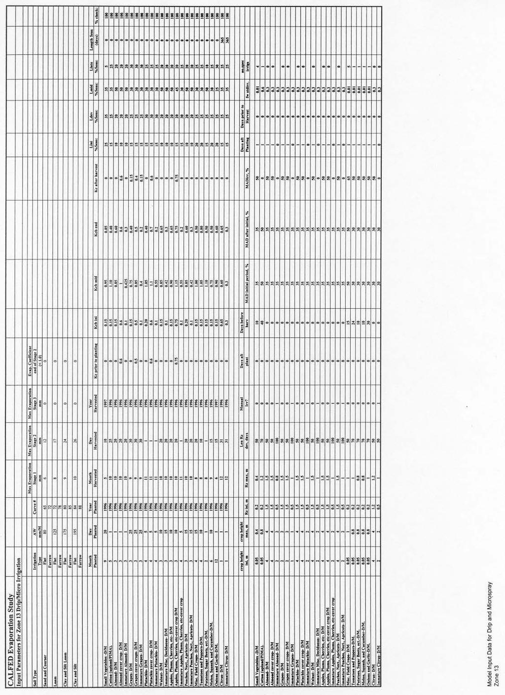
398

399

400

401

402

403

404

405

406

407

408

409

410

411

412

413

414

415

416

417

418

419

420

421

422

423

424

425

426

427

428

429 Appendix G. Bare Spots and Evaporation from Field Edges G-1 Reduction in Transpiration and Increase in Evaporation due to Bare Spots Throughout fields there are bare spots. These bare spots can be caused by many reasons including soil problems, weather, field slope and others. Because no field is perfect it is necessary to adjust evapotranspiration estimated by the FAO-56 Model based on these bare spots. A bare spot is classified in this study as a region within a field that is bare of plant life. Therefore there is no transpiration on this area, only evaporation. These bare spots do get irrigated at the same time as the crop on the field. It was necessary to estimate the evaporation from the bare soil based on irrigation scheduling for the crops. The FAO-56 Model schedules irrigation based on soil water depletion. In order to estimate evaporation from a bare surface within a cropped field it was necessary to schedule manual irrigations based what the program would have scheduled if a crop were using the water in the soil. If manual irrigations were not scheduled the program would have scheduled irrigations at a less frequent interval because the soil was bare of vegetation therefore using water at a lower rate. Five major crops in each of Zone 6 and 15 were chosen for this study. Zone 6 and 15 were chosen because they represent large areas and they are towards the extreme of each side of the ETo spectrum. The irrigation schedules for each crop-soil type category were obtained from the original FAO-56 Model program output file. These were applied to a new input file for the bare spots. The basal crop coefficients were set to 0. New FAO-56 Model runs were made for the bare soil based on each of the 5 crops irrigation schedules on the four soil type categories. Therefore a total of 20 runs were made for each zone. The input file for the bare soil runs was exactly the same as that for the crop except for setting Kcb = 0 (no transpiration) and the manual irrigation scheduling. CALFED/ARI Evaporation Study G-1 Irrigation Training & Research Center

430 G-1.1 Visual Analysis and Results from Previous Studies It is necessary to estimate how much land bare spots and decreased crop vigor effected. The ITRC has done studies in Imperial Irrigation District and Grasslands Region where individual fields were analyzed for bare spots and decreases in vigor. G Grasslands Region (West Side of the San Joaquin Valley) About 1800 slides of fields on the West Side of the San Joaquin Valley were examined and rated on the amount of bare spots observed in the summer of 1984 and Each slide was rated on the amount of bare soil surface (not including roads) and decreased vigor. It was estimated in the Grasslands Study that bare spots effected an average of 10% of the area and decreased vigor effected about 4-5% of the area. G Imperial Irrigation District A similar study was conducted in Imperial Irrigation District. In this study, 94 randomly selected 160 acre sections were analyzed. These fields were selected throughout the irrigation district and the analysis was done using aerial photos developed form multiple fly-overs of IID during a period of Feb. March of These areas were again rated based on the total amount of potentially cropped area that was without vegetation. The rest of the area was then rated on relative vigor. The results of this study estimated that 1.6% of the total potentially cropped area was bare of vegetation, and the average relative vigor rating was 0.88 (0 very poor vegetative uniformity, 1 very uniform vigor). The reduction in crop evapotranspiration (ETc) was estimated to be 6% for the IID study. This was determined based on a 1% decrease in vigor resulting in a 0.5% decrease in ETc. For this study it was assumed that 10% of the acreage in California was effected by bare spots and decreased vigor. CALFED/ARI Evaporation Study G-2 Irrigation Training & Research Center

431 G-1.2 Evaporation from Irrigated Agricultural Land in California Bare Spot Evaporation Extrapolation from Zone to Zone and Crop to Crop From the bottom 2 tables of Tables G-2 it can be seen that bare spots do not have a large impact on evaporation. Adjustments to evaporation were made based on these results for each zone and every crop in the study. Extrapolation to zones other than zone 6 and Zone 15 was necessary. Zones 1,3,4 and 8 adjustments resemble those of Zone 6 because of the similarities in weather. The other zones are similar to Zone 15 for the same reason. Minor adjustments were made based on rainfall. The more rainfall the more evaporation from precipitation and less irrigation needed, therefore the lower evaporation from irrigation water. It was assumed that crops not represented in Tables G-1 and G-2 would be adjusted based on the most similar crop that was represented. For example, corn was represented by cotton results, deciduous orchards were represented by the almond results. So from Tables G-2, Zone 15 almond annual total evaporation increases by inches per year. Therefore, it was assumed that apple, cherry, peach, nectarine, and all other orchard crops would also have an evaporation increase of inches per year. G-1.3 Adjustments Bare spots and decreased vigor cause a reduction in transpiration as well as an increase in evaporation. Total transpiration was reduced by 10%. Evaporation from irrigation water and precipitation as well as seasonal was increased by the amounts in the bottom tables of Tables G-2 depending on the zone and the crop. For example, if almonds in Zone 15 transpired 26 inches during the growing season and soil evaporation accounted for 8 inches, transpiration was reduced by 10% to 23.4 inches and evaporation was increased by 14.6% to 9.2 inches. The results in table G-2 were interpolated to crops within a zone by crop similarity and from zone to zone based on climate. These results are represented in results by irrigation system as well as the complete result tables. CALFED/ARI Evaporation Study G-3 Irrigation Training & Research Center

432 Tables G- 1. Results of the FAO-56 Model. The top 2 tables are the results of the evaporation from bare soil based on the crops typical year irrigation schedule. The bottom 2 tables are the results of the evaporation with for the non-bare soil. Cal-Fed Evaporation Study Bare Soil when Irrigated Zone 6 Bare Soil Zone 15 Bare Soil 1997 (Typical) 1997 (Typical) Evaporation Evap Irrig. Evap Precip Evaporation Evap Irrig. Evap Precip Annual Annual Annual Annual Annual Annual Crop inches inches inches inches inches inches Small Vegetables Almonds Cotton Grape Vines Grain and Grain Hay Original Evaporation with Crop Zone 6 Crop Zone 15 Crop 1997 (Typical) 1997 (Typical) Evaporation Evap Irrig. Evap Precip Evaporation Evap Irrig. Evap Precip Annual Annual Annual Annual Annual Annual Crop inches inches inches inches inches inches Small Vegetables Almonds Cotton Grape Vines Grain and Grain Hay CALFED/ARI Evaporation Study G-4 Irrigation Training & Research Center

433 Tables G- 2. The top 2 tables indicate the increase in annual evaporation for bare soil in comparison to annual evaporation. The bottom 2 tables represent the increase in evaporation, in inches, assuming that 10% of the land is effected. Cal-Fed Evaporation Study Increase in Evaporation for Bare Soil Zone 6 Bare Soil Zone 15 Bare Soil 1997 (Typical) 1997 (Typical) Evaporation Evap Irrig. Evap Precip Evaporation Evap Irrig. Evap Precip Annual Annual Annual Annual Annual Annual Crop Inches Inches Inches Inches Inches Inches Small Vegetables Almonds Cotton Grape Vines Grain and Grain Hay Assuming 10% of the acreage is effected [Inches of Evap increase from bare soil * % of land effected] = Total Inches of Evap increase Zone 6 Bare Soil Zone 15 Bare Soil 1997 (Typical) 1997 (Typical) Evaporation Evap Irrig. Evap Precip Evaporation Evap Irrig. Evap Precip Annual Annual Annual Annual Annual Annual Crop Inches Inches Inches Inches Inches Inches Small Vegetables Almonds Cotton Grape Vines Grain and Grain Hay CALFED/ARI Evaporation Study G-5 Irrigation Training & Research Center

434 G-2 Increases in Evaporation due to Edge Effects with Surface and Sprinkler Irrigation Adjustments were made to these tables that were not made on the regional summary tables by irrigation type. Adjustments for evaporation from field edges due to overspray from sprinkler irrigation and from open water surfaces in head ditches and tailwater ditches were accounted for in these results. The procedures used to estimate the magnitude of adjustments are laid out below. G Procedure for Calculating Field Edge Evaporation for Surface Irrigation Assumptions 1. Average field size is 80 acres 2. Wetted perimeter of head ditch is 7.04 ft 3. Wetted perimeter of tailwater ditch is 1.76 ft (Wetted perimeter values were obtained from Quinn, 1989) Figure G-1. Two scenarios for surface irrigation using head and tailwater ditches. The shaded area represents the ditches. Scenario 1 Scenario ' 2640' 80 acres 1320' 1.76' 7.04' acres 1320' 1.76' Scenario 1 Extra surface area wetted by the head ditch. Extra Acres Wetted per 80 acres = (7.04 *1320 )/(43560sqft/acre) = 0.231acres/ 80acres Extra surface area wetted by the tailwater ditch. Extra Acres Wetted per 80 acres = (1.76 *1320 )/(43560sqft/acre) = 0.053acres / 80acres CALFED/ARI Evaporation Study G-6 Irrigation Training & Research Center

435 Scenario 2 Extra surface area wetted by the head ditch. Extra Acres Wetted per 80 acres = (7.04 *2640 )/(43560sqft/acre) = 0.427acres/ 80acres Extra surface area wetted by the tailwater ditch. Extra Acres Wetted per 80 acres = (1.76 *2640 )/(43560sqft/acre) = 0.107acres / 80acres The two scenarios were averaged assuming that one scenarios use is the same as the other throughout California. The average extra acreage wetted per 80 acres, by a head ditch is 0.32acres/80acres and 0.08 acres/80acres by a tailwater ditch. The next set of assumptions was used to determine how much of the total surface irrigation is effected by extra evaporation due to open head and tailwater ditches. Not all surface irrigated area used open head ditches for delivery but can still have tailwater ditches and visa versa. These second set of assumptions are based on observations throughout California. These assumptions are; Field crops 1. 50% of the surface irrigation on field crops uses head ditches for delivery 70% of the 50% have tailwater ditches Therefore 35% of this acreage uses tailwater ditches 2. 50% of the surface irrigation on field crops uses gated pipe for delivery 50% of this 50% have tailwater ditches Therefore 25% of this acreage uses tailwater ditches 3. A total of 60% (35% + 25%) of surface irrigated field crops have tailwater ditches Tree and vine crops 1. 10% of the tree and vine crop surface irrigation acreage have tailwater ditches 2. 0% of the trees and vines throughout California use head ditches for water delivery. CALFED/ARI Evaporation Study G-7 Irrigation Training & Research Center

436 The evaporation increase will be proportional to the extra area wetted using open head ditches and tailwater ditches. Percentage of extra evaporation from open head ditches on field crop acreage = (50%/100)*(0.32acres/80acres) * 100 = 0.20% Percentage of extra evaporation from tailwater ditches on field crop acreage = (60%/100)*(0.08acres/80acres) * 100 = 0.05% Total percentage of extra area that has evaporation from field crop edges = (0.20% %) = 0.25% Total percentage of extra area that has evaporation from tree and vine crop edges = (10%/100)*(0.08acres/80acres) *100 = 0.01% Since the edge evaporation is not competing with transpiration from plants, this evaporation amount per unit area is greater than the evaporation from inside the field. An assumption will be made that evaporation from outside is 2 times more than the evaporation from the inside of the field. The total evaporation from irrigation water (Evap Irrig.), calculated by the FAO-56 Model, on field crops that were surface irrigate was increased by 0.5% (=0.25%*2) in these final results. Likewise, total evaporation from irrigation water on tree and vines crops that were surface irrigated was increased by 0.02% (=0.01%*2) in these final results. G Extra evaporation due to overspraying field edges during handmove and solid set sprinkler irrigation Assumptions CALFED/ARI Evaporation Study G-8 Irrigation Training & Research Center

437 1. The average field size is 80 acres 2. The extent of the overspray reaches 15 around the perimeter of the field 3. This overspray only occurs with handmove and solid set sprinkler irrigation, which accounts for approximately 80% of the sprinkler acreage Figure G- 1. The shaded area represents overspray around a handmove or solid set sprinkler irrigated field. 80 acre Field 15' 2640' 15' 1320' 15' 15' Extra acreage wetted by overspray Total acreage getting wet =[( )*( )]/(43560sqft/acre) = acres being wetted Extra acreage being wetted = 81.37acres 80acres = 1.37 acres/80acres being wetted by overspray Percentage of extra area that has evaporation due to overspray on sprinkler irrigated fields = (80%/100) * (1.37acres/80acres) = 1.4% It will be assumed again that 2 times more evaporation from irrigation water will occur on the edges of the field than will occur inside of the field. Therefore calculated evaporation from irrigation water on sprinkler irrigated fields was increased by 2.8% (=1.4%*2) to account for overspray. CALFED/ARI Evaporation Study G-9 Irrigation Training & Research Center

438 Sources of Information Evaporation from Irrigated Agricultural Land in California 1. Water Study Team. Imperial Irrigation District Water Use Assessment for the Years March Received via Freedom of Information Act. 2. ITRC. Grasslands Basin Irrigation and Drainage Study. May Ouinn, N.W.T., R.S. Smith, C.M. Burt, T.S. Slavin, S.W. Styles, A. Mansoubi Water seepage from unlined ditches and reservoirs. California Agriculture. v43, no. 6. CALFED/ARI Evaporation Study G-10 Irrigation Training & Research Center

439 APPENDIX H REALITY CHECK OF ET VALUES H-1 ETo Zone 15 Reality Check In order to assess the assumptions used in the evapotranspiration model, the annual crop evapotranspiration amounts calculated by the FAO 56 Model were compared to more detailed crop evapotranspiration numbers that had been developed by others for some crops in specific regions in California. Such a reality check is very necessary. There are major differences in published Kc values for a single crop (Kcb values are rarely published). The final computation of Kc values within the ITRC procedure depends upon assumptions based on published data related to frequency of irrigation, the existence of under-irrigation, and growing season lengths, but which may be incorrect. It is not unusual to find differences of 40-50% in published ET estimates for crops such as beans and melons in the same region. H-1.1 ETo Zone 15 Comparison ETo Zone 15 was used for one the comparisons. Modeled ETc values were compared to ETc (growing season) estimates from Westlands Water District (WWD), estimates previously made by ITRC for Panoche Water District, estimates of necessary delivered irrigation water made by Panoche WD farmers, and delivered irrigation water data from Broadview WD. This was an important region to check because the limited allocation of water may result in crop stress due to deficit irrigation (applying less water then the crop potentially would use). It would be an error if mistaken assumptions led to the model calculating more evapotranspiration than water even being supplied to the crop. Westlands Water District publishes information on crop evapotranspiration (ETc) during the growing season. The WWD values ignore evaporation and any weed transpiration during other periods of the year. The WWD values do not attempt to distinguish between irrigation water and rain water. The values were obtained from neutron probe readings taken within the active root system. For example, for drip irrigated almonds, the neutron probe site would be located within the wetted area supplied by an emitter. For drip irrigation of almonds (the majority of almonds in WWD), it was assumed that if the soil moisture content remained constant CALFED/ARI Evaporation Study H-1 Irrigation Training and Research Center

440 for a period of time, then the applied water equaled the ET. The theory behind this was that if the applied water was less than necessary, the neutron probes would measure a decline in moisture content, and if an excess amount was applied, the moisture content would increase. There are some potential weaknesses to this method, including: - Neutron probes cannot accurately measure moisture content changes that occur close to (within 6 of) the soil surface - a major area of interest for this study. - Consistent over-application of irrigation water will provide an appearance of consistent soil moisture content after a period of time. Twice weekly measurements of a neutron probe will not provide data that shows the deep percolation, whereas hourly readings by other devices, such as the Sentek soil moisture measurement unit, would show such deep percolation. - It is possible for the soil to stabilize at fairly dry moisture content with under-irrigation. - The neutron probes may not have been deep enough to notice all soil moisture changes. For example, the access tubes were generally limited in length to 6, but almond and cotton roots extend below 6 on many soils. In spite of these weaknesses, the WWD data is supported by internal (WWD) reality checks of applied irrigation water and effective rainfall depths. Therefore, the WWD is considered to be reasonably accurate - certainly not within 5% accurate, but nevertheless better than much other available data. The second source of evapotranspiration numbers compared against Zone 15 modeled evapotranspiration were related to Panoche WD (PWD). There are two sets of values for PWD - first, some ETc estimates from an earlier study done by ITRC, and second, applied water allocations for Panoche Water District (PWD). The applied water allocations for PWD are particularly important because those numbers have been developed by PWD in close cooperation with its farmers, who have relatively high on-farm irrigation efficiencies and who have good records of how much water they need to grow crops under different conditions. For example, in PWD the farmers clearly understand that areas with a high water table require less applied water than areas without a high water table; farmers who farm in both areas have a good sense for the relative difference in gross irrigation water requirements. Broadview WD also has excellent applied irrigation water data for its crops. This data was used as part of the reality check, as well. The reality check recognized that BWD has a high water table that may be due in part to water entering from upslope irrigators. The Panoche Water District ETc and the WWD ETc values are not directly comparable numbers because PWD ETc was based on an annual basis, while WWD ETc was based on the growing season. For this study comparison, ITRC computed PWD ETc values for both annual and growing periods using the FAO 56 Model. The annual ETc was compared to the Panoche Water District ETc and the growing period ETc was compared to CALFED/ARI Evaporation Study H-2 Irrigation Training and Research Center

441 the Westlands Water District ETc. Table H-1 shows the comparisons between Zone 15 Model ETc, Panoche ETc, and Westlands ETc. H-1.2 Discussion The first check was for surface irrigated almonds. The management allowable depletion used for irrigation scheduling was increased from 50% to 75% on average for all 4 soil types in order to decrease the crop seasonal evapotranspiration to match WWD ETc values. The annual ETc values from the model, once the MAD was increased, match well with the annual Panoche ETc values. This was the case for every crop that was checked. Table H-2 shows the new MAD used for each crop after the reality check was completed. Crops such as apples and citrus did not have comparison values because they are not major crops in that region. Tree and vine crops with cover crops were given the same MAD to schedule irrigation as the same crop grown without a cover crop. CALFED/ARI Evaporation Study H-3 Irrigation Training and Research Center

442 Table H-1. ETo Zone 15 Reality Check. Surface irrigation during a typical year. CALFED/ARI Evaporation Study H-4 Irrigation Training and Research Center

443 Table H-2. New MAD used to schedule irrigations with surface and sprinkler irrigation as a result of the reality checks in Zone 15. MAD used for Irrigation Scheduling Crops % Small Vegetables -Furrow- S 65 Alfalfa Hay mature-border-s 60 Cotton (upland/pima)-furrow.-s 65 Almond- Border-S 75 Almond cover crop- Border-S 75 Corn- Furrow-S 70 Grapes- Furrow-S 75 Grapes cover crops- Furrow-S 75 Pistachio- Border-S 70 Pistachio cover crop- Border-S 65 Misc. Decidous- Border-S 75 Apples, Plums, Cherries, etc- Border-S 75 Apples, Plums, Cherries, etc-cover crop Border-S 75 Peaches, Nect., Apricots- Border-S 70 Grain and Grain Hay Border.-S 70 Rice-S 50 Safflower and Sunflower-S 65 Misc. Field Crops- Furrow-S 70 Pasture-S 65 Tomatoes and Peppers-Furrow.-S 70 Potatoes, Sugar Beets, ect.-furrow.-s 65 Melon, Squash, and Cucumber-Furrow.-S 65 Onions and Garlic-Furrow.-S 70 Citrus- Border-S 65 Idle- Border-S 0 H-2 ETo Zone 18 Reality Check A very detailed crop evapotranspiration study was previously done for Imperial Irrigation District (IID) for the time period of The crop evapotranspiration values were rigorously obtained for the IID Study using the FAO 56 approach, with grower interviews to obtain good irrigation scheduling and cropping method information. Within the IID Study, multiple planting and harvest dates were modeled and crop rotations were taken into account. But the major factor which gives a high level of confidence to the earlier study results was that there was a very reliable reality check on the ETc values - the Imperial Valley is an excellent lysimeter. Therefore, the earlier study had excellent inflow and outflow measurements, which left ET as the remainder. As a result, the weather-based ET estimate (including all values of ET such as water surface E, crop ETc, etc.) CALFED/ARI Evaporation Study H-5 Irrigation Training and Research Center

444 could be fine-tuned to closely match a known true value. The quality of the estimated crop evapotranspiration in the IID Study is considered very high; therefore, it was used to check this Evaporation Study s ETc values. Direct comparisons were made between the annual IID Study values and the annual Evaporation Study values and can be seen in Table H-3. Adjustments were made to the management allowable depletion (MAD) that was used to schedule irrigations if the Evaporation Study values were higher than the IID Study values. The values were close and only a few adjustments had to be made. This was due to the fact that some of the IID Study input parameters were the same as the Evaporation Study input parameters to make the ITRC runs. The MAD s and average planting and harvest dates were obtained from the same sources of information as in the earlier study. Pasture and miscellaneous grasses was one category that was altered for the comparison. The MAD used to schedule irrigations was increased to about 70% to reduce the ETc value. The MAD values for grain and grain hay were increased to 65% to match the IID Study values. CALFED/ARI Evaporation Study H-6 Irrigation Training and Research Center

445 Table H-3. ETo Zone 18 Reality Check. Surface irrigation during a typical year. CALFED/ARI Evaporation Study H-7 Irrigation Training and Research Center

446 H-3 Sources of Information 1. Westlands Water District. 1999, Water Management Plan, pg ITRC Evapotranspiration Estimates for Firebaugh-Los Banos Area (Panoche Water District) 3. Broadview Water District. Total Applied Water values for major crops in the District Water Study Team. Imperial Irrigation District Water Use Assessment for the Years March Received via Freedom of Information Act. CALFED/ARI Evaporation Study H-8 Irrigation Training and Research Center

447 ITRC Report No APPENDIX I RESULTS BY IRRIGATION SYSTEMS I-1 Evapotranspiration Results by Irrigation System The FAO-56 Model was used to estimate the evapotranspiration from crops grown using three irrigation regimes: surface, sprinkler, and drip/micro. The acreage of each irrigation type per crop per soil type was estimated as described in Appendix D. The results presented in this Appendix were originally daily output from the FAO-56 Model. The following is a summary of how these numbers were generated. For more details on how the model generates these results, see Appendix B. 1. The FAO-56 Model Quick Basic program used a data input file. Different data input files were made up for every zone, for each of the 3 irrigation system categories. In each of these input files there was information on the cropping methods, irrigation methods and soil information (see Appendix F). Therefore, a total of 39 input files were used (13 zones x 3 irrigation categories). Each irrigation category was looked at separately. 2. Once the FAO-56 Model Quick basic program output one of the 39 output files, it was necessary to do several summaries. The results were first summed in a separate Quick Basic program by month and presented as the millimeters of water per crop-soil-irrigation system combination. 3. There are about 120 different crop-soil combinations, depending on the zone. With 3 irrigation categories, there are about 360 different crop-soil-irrigation combinations for each zone. This was brought into an Excel spreadsheet, where it was then summarized in millimeters on an annual basis using a pivot table report. This study covered 3 years: 1997, 1998, and The millimeters of annual water per crop-soil-irrigation combo was then converted to a depth in feet and multiplied by the estimated acreage with that combination. This delivered the acre-feet of water use by each crop on each soil for each irrigation category. 5. The volume of evapotranspiration from each of the 4 soil type categories for each crop were then added together, resulting in the acre-feet of water by crop-irrigation system combination. These are presented as the acre-feet tables for each zone and irrigation method attached to this appendix. CALFED/ARI Evaporation Study I-1 Irrigation Training and Research Center

448 ITRC Report No These acre-feet values were then divided by the number of acres that each combination covered in each zone (this acreage is the first column in each acre-ft table). This value was multiplied by 12 inches per foot, giving the second set of summary tables, which are in inches for each zone and irrigation method. I-1.1 Results for Surface Irrigation Surface irrigation includes furrow, borderstrip, basin, and combination sprinkler-furrow. The combination category was placed in the surface irrigation type because the sprinkler portion of the irrigation is generally done during the early part of the season and for pre-irrigation. For the majority of the season, furrow irrigation is used. One of the main reasons for having the sprinkler irrigation category is to estimate the amount of evaporation from the wet plant surface. If sprinklers are used during the early part of the growing season only, the evaporation from the wet plant surface is negligible because there is little or no plant surface for this potential evaporation. As for evaporation from the soil surface, it is handled the same for both furrow and sprinkler early in the season. Pre and early season irrigations generally wet the entire surface for both irrigation types. This is done for leaching or seed germination. Therefore, since early season irrigations are always set in the model to wet the entire surface, the model handles both irrigation types the same. The results for surface irrigation are in the first set of attached tables. The first 42 tables are in acre-ft and the second 39 are in inches. The first 3 tables are the total water use on surface irrigated land for 1997, 1998, and The rest of the tables are the results of each individual zone. I-1.2 Results for Sprinkler Irrigation Sprinkler irrigation includes handmove, solid set, center pivot, side-roll and linear move systems. Planting, leafout, and harvest dates, as well as soil properties, were assumed to be the same for sprinkler and surface irrigation. Evaporation from sprinkler irrigation in these results includes evaporation from a wet plant surface (see Attachment B) and evaporation from a fraction of wetted soil equal to 1.0. Attachment F identifies the fraction of soil wetted (fw) by different irrigation types for different crops. In this report it was assumed that sprinkler irrigation has a fw=1.0. The results of sprinkler irrigation runs are in the second set of tables. The first 42 are in acre-ft and the next 39 are represented in inches. The first 3 tables in this section are the total water use in acre-ft for sprinkler irrigated land in California. The rest of the tables are results by ETo Zone. I-1.3 Results for Drip/Micro Irrigation The major differences in drip/micro are the fraction of wetted area, assumed to be about 0.3, and lower MAD for more frequent irrigations. The amount applied per irrigation of course is smaller but the number of irrigations increases. For this report it was assumed that the amount of water stress did decrease with drip/micro, increasing the amount of evapotranspiration. The amount of stress was decreased and the number of irrigation increased by lowering the MAD s. One MAD is used to schedule irrigations based on soil water CALFED/ARI Evaporation Study I-2 Irrigation Training and Research Center

449 ITRC Report No content. The other MAD is used to determine at what magnitude water stress begins, in relation to root zone depletion. These were both lowered, although the MAD that schedules irrigations was lowered more. This resulted in less overall stress and more frequent irrigations. The results of drip/micro irrigation runs are in the third set of tables. The first 42 are in acre-ft and the next 39 are represented in inches. The first three tables in this section are total water use on drip/micro irrigated land in California as a whole. The rest of the tables are the results by zone. An explanation of these results can be found in Appendix J Sections J-1.2 J-1.7. Files: CALFED Surface Evap summary (acre-ft).xls CALFED Surface Evap summary (inches).xls CALFED Sprinkler Evap summary (acre-ft).xls CALFED Sprinkler Evap summary (inches).xls CALFED drip Evap summary (acre-ft).xls CALFED drip Evap summary (inches).xls (The excel spreadsheets will be available as part of an ITRC/CALFED report to the general public in Fall Following are 3 sample spreadsheets.) CALFED/ARI Evaporation Study I-3 Irrigation Training and Research Center

450 ITRC Report No

451 ITRC Report No

452 ITRC Report No

453 APPENDIX J ETC AND EVAPORATION FINAL RESULTS J-1 Summary Tables The first three tables attached to this appendix make up the overall evaporation and evapotranspiration summary table. The next 39 tables are the modeled evaporation volume summaries for the study zones. The last 39 tables are the summaries for the individual zones in acre-inches per acre (inches). The acre-feet results are the sum of the acre feet results for each irrigation type (surface, sprinkler and drip/micro) for each zone (from Appendix I). The results represented as inches are the average inches of water use within each zone. The inch results are calculated by dividing the total acre-feet of water use by the total acreage of that crop in each zone. The inches are therefore weighted based on the acreage of irrigation types for each crop. These final results have accounted for variations in soil type, irrigation regimes, weather, bare spots, crop stress, crop maturity, and as will be discussed below, evaporation from open head ditches, tailwater ditches, and sprinkler overspray for irrigated agriculture acreage throughout California. J-1.1 Irrigation Season Evapotranspiration These results represent the evaporation and transpiration throughout the growing season of the crop in question. The growing or irrigation season starts on the planting date and ends on the harvest date. J-1.2 Offseason Evapotranspiration The offseason is the period from harvest of one year to planting of the next year. It was assumed that for annual crops and deciduous perennial crops without a cover crop the offseason would consider evaporation from a bare soil. Trees with a cover crop consider cover crop transpiration and evaporation. Alfalfa and citrus irrigation (growing) seasons are considered to be 365 days per year. Therefore, they do not have an offseason. CALFED Evaporation Study J-1 Irrigation Training and Research Center

454 J-1.3 Evapotranspiration Without Stress There are two columns for annual evapotranspiration. The first is the crop's potential evapotranspiration, or the amount of evapotranspiration that would occur if the crop was irrigated on a perfect irrigation schedule not allowing crops stress. Mathematically it is calculated as: where, ETc w/o Stress = ETo*[Kcb + Ke] (See Appendix B) ETo Grass reference evapotranspiration Kcb Basal Crop Coefficient Ke Evaporation Coefficient J-1.4 Actual Annual Evapotranspiration Actual annual evapotranspiration (ETc Actual) is the evapotranspiration during the offseason plus the evapotranspiration of the irrigation season. This value includes the reduction in transpiration due to water stress. Water stress occurs when imperfect scheduling results in under-irrigation, and when there is deficit irrigation. It is literally impossible to schedule irrigations perfectly. Generally, there will either be overirrigation or under-irrigation. Deficit irrigation occurs because growers are not allotted as much water as is necessary to meet potential ETc. This is because, in many areas of California, water is in short supply (see Appendix H for more detailed discussion on how the amount of crop stress was derived). J-1.5 Amount of Irrigation Evapotranspiration and Precipitation Irrigations are scheduled in the model based on the management allowable depletion and the root zone depletion (see Appendix B). Therefore, the irrigation water applied represents the irrigation water used as evapotranspiration because it meets the root zone depletion exactly. It is assumed that the irrigation water applied by the program (This is not a gross irrigation amount and should not be assumed to be the amount of irrigation water that should be applied to a crop. There are many other factors including, but not limited to, application efficiency, leaching requirements and distribution uniformity) equals the amount of irrigation water evapotranspiration (Irrigation ET). Precipitation was obtained from CIMIS stations throughout California. The actual amount of precipitation used in each zone was the average of values from all stations within the zone. J-1.6 Evaporation from the Net Irrigation and Precipitation The total evaporation each day was partitioned into evaporation from irrigation water or from precipitation. The explanation of how evaporation from irrigation (Evap Irrig.) and precipitation (Evap Prec) was separated can be found in Appendix B. CALFED Evaporation Study J-2 Irrigation Training and Research Center

455 Files: CALFED Complete Evap Summary (Acre ft).xls CALFED Complete Evap Summary (Inches).xls (The excel spreadsheets will be available as part of an ITRC/CALFED report to the general public in Fall Following are 3 sample spreadsheets.) CALFED Evaporation Study J-3 Irrigation Training and Research Center

456

457

458