Conditional Random Fields, DNA Sequencing. Armin Pourshafeie. February 10, 2015

Transcription

1 Conditional Random Fields, DNA Sequencing Armin Pourshafeie February 10, 2015 CRF Continued HMMs represent a distribution for an observed sequence x and a parse P(x, ). However, usually we are interested in the parse that the sequence we have implies (P ( x)). We can model this probability using CRF s Definition P ( x) = exp(p i=1... x wt F ( i, i 1,x,i)) P exp(p i=1... x wt F ( i 0, 0 i 1,x,i)) where F : (state, state, observations, index)2 R n is called the local feature mapping. Note that this form is more general than HMM s. In particular, since we are looking at entirety of x we can model events that we couldn t using HMM s. w 2 R n is the parameter vector (a set of weights) Relationship to HMM s From the definition, we can notice that CRF s can model a greater set of systems. they can look at the entire set of emissions x. In particular any HMM can mapped to a CRF. For a HMM we have x X log P (x, ) = log P ( 0 )+ log P ( i i 1 ) + log P (x i i ) For a CRF, we can define weights x i=1 X = log a log a( i 1, i ) + log e i (x i ) i=1 1

2 and feature vector F ( i, i 0 1 log a 0 (1). log a 0 (K) log a 1 (1) w =. 2 R n log a K (K) log e 1 (b 1 ) B A log e K (b M ) 0 1 1{i =1, i 1 =1}. 1{i =1, i 1 = K} 1{ i 1 =1, i 1 =1} 1,x,i)=. 2 R n 1{ i 1 = K, i = K} 1{x i = b 1, i =1} B A 1{x i = b M, i = K} Where 1{x} is the indicator function for x. This gives log probability x X log P (x, ) = w T F ( i, i i=1 1,x,i) From which we can get the conditional probability P x P (x, ) exp i=1 P ( x) = = wt F ( i, i 1,x,i) P P (x, ) P exp P x i=1 wt F ( i, i 1,x,i) This shows: HMM ( CRF 0 s HMM parameter vectors have restrictions that are not present in CRF. for instance in an HMM P i a 0i = 1 (since this refers to probability of transition.) but in CRF parameter vectors only need to be positive. CRFs can have features that HMM s cannot have. 2

3 For an HMM the feature vector is F ( i, i 1,x i,i) HMM s can only generate each observation once whereas CRF s can have features dependent on x i 1,x i+1 We could in principle define a very large set of features but this will require a very large training data set. The down side is that CRF s don t model the observations. i.e. They are not generative models. CRF needs categorized data for learning. Basic questions for CRF s Just like HMM s, there are 3 important questions we would like to answer. Evaluation: Given a sequence of observations (x), andasequenceofstates ( ), what is P ( x)? Decoding: Given a sequence of observations (x) what is the maximum probability sequence of states = arg max P ( x) Learning: Given a CRF, compute the weights that maximize the likelihood of given x. w ML = arg max w P ( x, w) Decoding Decoding can be done with the Viterbi for CRF s Using P ( x) given earlier, we can write arg max P ( x) = arg max = arg max exp( X = arg max exp( P i=1... x wt F ( i, i P exp(p i=1... x wt F ( i 0, 0 i X i=1... x i=1... x w T F ( i, i w T F ( i, i 1,x,i) 1,x,i)) 1,x,i)) 1,x,i)) Where we have used monotonicity of exp to get from the second to the third line. Now, we can easily extend the Viterbi algorithm using V k (i) = max j w T F (k, j, x, i)+v j (i This is very similar to the Viterbi for HMM s however, there is no emission and transmission probabilities, and now we have a dot product of the weights with the feature vector. 1) 3

4 Figure 1: Note that the features in the CRF can depend on any position in x but DP depends only on the previous state. We could extend the forward/backward algorithm to compute the partition function. We can intuitively justify this algorithm. Even though the features could depend on any x, given that at time i we end up in state k, wecanseparately maximize the scores to the left and to the right. Since x is fixed, the parse to the left and to the right are do not effect each other except for the fact that they have to end/start at k. Learning Note that log P ( x, w) is both differentiable and convex. Therefore we can use gradient descent and be sure to find the global solution. (Contrast this with Baum-Welch which gives the local solution) In order to run gradient descent (ascent) we first compute the partial derivatives w.r.t w j log P ( x, w) =F j (x, ) E 0 p( 0 x,w)[f j (x, 0 )] Where E 0 p( 0 x,w)[f j (x, 0 )] is the expected value of jth feature given the current parameters and F j (x, ) is the value of the jth feature given the correct parameters. Notice that the if the true value of the jth feature is higher than the mean calculated by our parameters this derivative is positive, which will increase w j and if the case is reversed then the derivative is negative which will decrease w j upon iteration. 4

5 Figure 2: DNA Sequencing Background DNA sequencing allows us to determine the order of nucleotides in an individuals DNA. The DNA is consisted of about 3 billion base pairs. The Human Genome project started in 1990 and took more than 10 years (2001 for the first draft) and over $3 billion dollars to complete. During the 1990 s two separate programs attempted to sequence the human genome. The public effort (Human Genome Project) collected DNA from 12 anonymous regional individuals. The private effort by Celera Genomics attempted to sequence the DNA of the CEO Dr. Craig Venter. At the end of the day, any two individual s DNA sequence is more than 99.9 % similar so either sequence could be fairly representative of the Human population. Why is the Human genome so similar? On average, only 1 out of 1000 letters of two individuals is different. In contrast, in Ciona savignyi, two individuals may have up to 10% difference in their DNA. This low polymorphism rate is related to the population size. For most of human history, human population has been very small (~10,000 individuals living in Africa). At a certain choke point, the human population reduced to ~1000. This small population interbred with individuals with very similar genomes which reduced the genetic variation. With the expansion of human population in recent history, we are acquiring some rare mutations. In particular, we can compute the heterozygosity of a population using h = 4Nµ 1+4Nµ where N is the population size ( 104 for most of human history) and µ mutation rate (10 8 ). Polymorphism comes in many forms. The most common is Single Nucleotide Polymorphism (SNP) which is when a single base pair is different among two individuals. Another kind of polymorphism is copy number variation (CNV) which is referred to the case where a large region of DNA is duplicated more or 5

6 less than usual. Cost While the Human Genome Project cost 3 Billion dollars for a single sequence, the cost has been dropping sharply. With about $1000 per sequence in This is good news as it opens up the possibility of sequencing different species, different people or even different tissues of the same person. Sequencing Old technology, Sanger vectors This method was developed by the biochemist Frederick Sanger, who won two Nobel prizes for his work in DNA sequencing. This method was the dominant technology for ~25 years after it s invention in 1977 and has more recently been replaced by Next-Generation sequencing. In this method: 1. We break the DNA into fragments of different sizes by sonication, (each fragment is a few thousands base pairs). 2. Each small fragment then is copied many times. In order to copy the fragments, each piece is inserted into a known region of a circular, self-replicating piece of genome known as cloning vector (bacterium, plasmid). After insertion, the cloning vector is replicated many times using cellular DNA-replication machinery. Since the location of the DNA fragment is known, we can cot it from the cloning vector. 3. Next we determine the ordering of nucleotides within the copied pieces. In order to do this the DNA is placed in a solution so it can replicate however, the solution will have small concentration of base pairs similar to ACGT which are 6

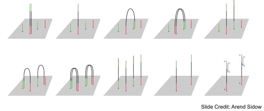
7 Figure 3: fluorescent and terminate the copying process. This produces many substrings of the original DNA each starting from the beginning but ending at different points with a fluorescent base-pair. These subcopies are then organized based on length using electrophoreses and the base pairs can be read using the fluorescent base-pairs at the end. Illumina In this method, 1. The DNA is fragmented and tagged with a different adaptor at each end. 2. Each fragment is then amplified in a flow cell. The flow cell contains receptors that are complementary to the tags on the DNA. The DNA fragment will attach to these tags. Then a complement of the fragment is produced and the original fragment is washed away. The complementary fragment then clones itself through bridge amplification. In this method, the fragment bridges so the other end tag is connected to the other type of receptor. Then the fragment is cloned and the two clones are separated so that one version of the clone is on each receptor. This process is then repeated many times. At the end, the reverse strands are washed off. 3. Finally, the DNA is sequenced using Sequencing by Synthesis. In this method, the complement of the DNA is made one base at a time. Each base has a fluorescent tag and can be read after it is attached. This entire sequencing process is done in a massively parallel way. Assembly After sequencing, the reads need to be assembled into a DNA sequence. There are two types of assembly problems 1. De Novo Assembly 2. Resequencing 7

8 Figure 4: Figure 5: 8

9 Figure 6: Clustering De Novo Assembly Figure 7: Linking De Novo Assembly refers to the problem of assembling from scratch. For example, assembling the first human DNA. In this method, we try to cover each region with high redundancy, then we will overlap and extend each read. Here, coverage is defined as the expected number of reads per region and is given by: C = NL/G Where N: is the number of reads, L is the length of reads and G is the length of the genome. Repeat problem One major problem with the sequence reconstruction is the problem of repeats. While repeats are not common in lower organisms (~5% for bacteria) in mammals they are very common (~50%) repeats are dangerous because they could cause two faraway parts of the DNA to concatenate. Of course, repeats that are shorter than the length of a read, are not a problem. There are two usual methods to deal with the repeat problem: 1. Clustering the reads: Clustering the reads to different regions will reduce the chance of having long repeats in each cluster. (Figure 6) 2. Linking the reads (Figure 7) 9