CHAPTER 6. Genetic Linkage and Mapping in Eukaryotes. (Brooker Genetics 5 th ed) 염색체의위의모든유전자는연관되어있다 멘델의유전법칙에위배되는결과도출

Transcription

1 CHAPTER 6 Genetic Linkage and Mapping in Eukaryotes (Brooker Genetics 5 th ed) 염색체의위의모든유전자는연관되어있다 멘델의유전법칙에위배되는결과도출 유전자지도작성? -F1 heterozygote 의 testcross - 교차에의한염색체교환 -Nonparental type recombinant 자손생성 -Recombinant type 의개체수측정 -RF(recombination frequency) 측정 - 두유전자간의거리계산 ( 추정 ) 1

2 2

3 INTRODUCTION Each species of organism must contain hundreds to thousands of genes Yet most species have at most a few dozen chromosomes Therefore, each chromosome is likely to carry many hundred or even thousands of different genes ( 수백 - 수천개의유전자가한개의염색체라는한배를타기때문에감수분열동안동행할것이므로독립의법칙을거스르게된다.) The transmission of such genes will violate Mendel s law of independent assortment 6.1 LINKAGE AND CROSSING OVER In eukaryotic species, each linear chromosome contains a long piece of DNA A typical chromosome contains many hundred or even a few thousand different genes The term synteny means two or more genes are located on the same chromosome and are physically linked The term linkage has two related meanings 1. Two or more genes can be located on the same chromosome 2. Genes that are close together tend to be transmitted as a unit 3

4 Chromosomes are called linkage groups They contain a group of genes that are linked together The number of linkage groups is the number of types of chromosomes of the species For example, in humans 22 autosomal linkage groups An X chromosome linkage group A Y chromosome linkage group Q: 동일염색체위의유전자는 linked 되어있는데도불구하고생식세포 (germ cells) 의감수분열때어떻게독립적으로배우자세포 (gamete) 속으로분리되어이동할있을까? Copyright The McGraw-Hill Companies, Inc. Permission required for reproduction or display 4

5 Bateson and Punnett Discovered Two Traits That Did Not Assort Independently In 1905, William Bateson and Reginald Punnett conducted a cross in sweet pea involving two different traits Flower color and pollen shape This is a dihybrid cross that is expected to yield a 9:3:3:1 phenotypic ratio in the F 2 generation However, Bateson and Punnett obtained surprising results Refer to Figure 6.1 Figure 6.1 The data showed that independent assortment does not always occur 5

6 Q: How to interpret their data by Bateson and Punnett? They suggested that the transmission of the two traits from the parents was somehow coupled The two traits are not easily assorted in an independent manner ( 두형질은어떤이유에든연결되어있어독립적인방식으로쉽게분리되지못하는것으로추정함 ) However, they did not realize that the coupling is due to the linkage of the two genes on the same chromosome Copyright The McGraw-Hill Companies, Inc. Permission required for reproduction or display 6

7 Relationship between linkage and crossing over Crossing Over May Produce Recombinant Phenotypes In diploid eukaryotic species, linkage can be altered during meiosis as a result of crossing over Crossing over Occurs during prophase I of meiosis at the bivalent stage Non-sister chromatids of homologous chromosomes exchange DNA segments Figure 6.2 illustrates the consequences of crossing over during meiosis Figure 6.2 Copyright The McGraw-Hill Companies, Inc. Permission required for reproduction or display 7

8 These are termed parental or nonrecombinant cells These haploid cells contain a combination of alleles NOT found in the original chromosomes This new combination of alleles is a result of genetic recombination These are termed nonparental or recombinant cells Figure 6.2 8

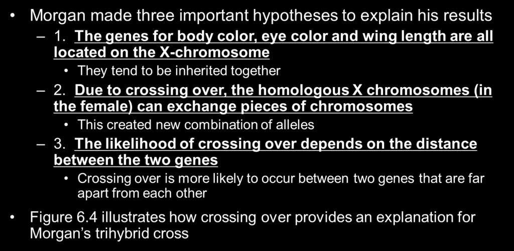
9 Morgan Provided Evidence for the Linkage of Several X-linked Genes The first direct evidence of linkage came from studies of Thomas Hunt Morgan Morgan investigated several traits that followed an X-linked pattern of inheritance Figure 6.3 illustrates an experiment involving three traits Body color Eye color Wing length Copyright The McGraw-Hill Companies, Inc. Permission required for reproduction or display 9

10 Figure 6.3: Morgan s trihybrid cross involving three X-linked traits in flies 10

11 However, Morgan still had to interpret two key observations 1. Why did the F 2 generation have a significant number of nonparental combinations? 2. Why was there a quantitative difference between the various nonparental combinations? 11

12 Figure 6.5 (Different proportions of recombinant offspring) 12

13 Figure 6.5 (a) No crossing over, parental offspring These parental phenotypes are the most common offspring (b) Crossover between eye color and wing length genes, fairly common These recombinant offspring are not uncommon (fairly common) because the genes are far apart 13

14 Figure 6.5 (c) Crossover between body color and eye color genes, uncommon These recombinant offspring are fairly uncommon because the genes are very close together (d) Double crossover, very uncommon These double recombinant offspring are very unlikely, 1 out of 2,205 14

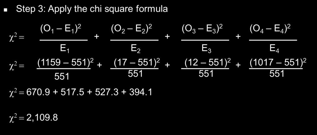
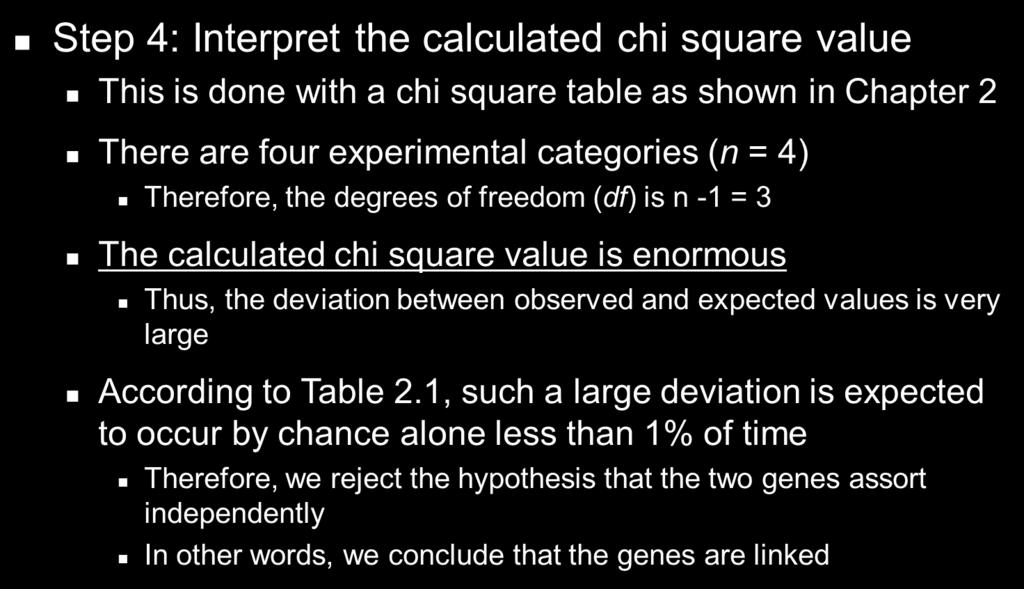
15 Chi Square Analysis This method is frequently used to determine if the outcome of a dihybrid cross is consistent with linkage or independent assortment Let s consider the data concerning body color and eye color An example of a chi square approach to determine linkage is shown next 15

16 Cross: (X y+w+ X yw ) X (X yw Y) The probability of each phenotype is equal as ¼ since the cross is testcross 16

17 17

18 헉!!! 2,

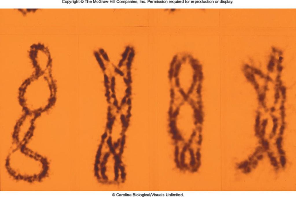
19 Creighton and McClintock Experiment To obtain direct evidence that genetic recombination is due to crossing over, Harriet Creighton and Barbara McClintock used the following strategy 1. They made crosses involving two linked genes These crosses yielded parental and recombinant offspring 2. They observed microscopically the chromosomes in the parents and offspring The parental chromosomes had some unusual structural features (See Figure 6.6) They wanted to see if there was a correlation between The occurrence of recombinant offspring with Microscopically observable exchanges in segments of homologous chromosomes Copyright The McGraw-Hill Companies, Inc. Permission required for reproduction or display 19

20 Creighton and McClintock focused on the pattern of inheritance for traits in corn In previous cytological examinations of corn, they found a chromosome number 9 that had two abnormalities 20

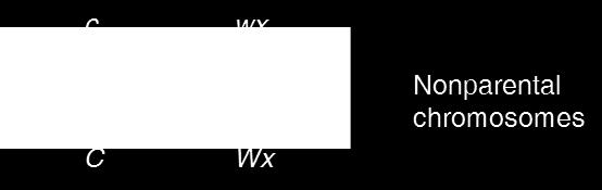
21 Creighton and McClintock reasoned that a crossover involving a normal and an abnormal chromosome 9 would yield A chromosome that had either a knob or a translocation, but not both These chromosomes are distinguishable from the parental chromosomes Colorless Starchy Colored Waxy c C Wx wx Parental chromosomes Crossing over Colorless Waxy Colored Starchy Figure 6.6 c C wx Wx Nonparental chromosomes (b) Crossing over between normal and abnormal chromosome 9 21

22 The Hypothesis Offspring with nonparental phenotypes are the product of a cross-over This cross over created nonparental chromosomes via an exchange of segments between homologous chromosomes Testing the Hypothesis Refer to Figure 6.7 Copyright The McGraw-Hill Companies, Inc. Permission required for reproduction or display 22

23 23

24 (Parental type) (Parental type) (Nonparental type) (Nonparental type) (Nonparental type) 24

25 Interpreting the Data Creighton and McClintock were interested in whether crossing over occurred in parent A It was the one heterozygous for both genes (CcWxwx) The number of gametes produced by the parents is as follows Parent A C wx (nonrecombinant) c Wx (nonrecombinant) C Wx (recombinant) c wx (recombinant) Parent B C Wx c wx (cc Wxwx) By combining these gametes into a Punnett square, the following types of offspring can be produced Copyright The McGraw-Hill Companies, Inc. Permission required for reproduction or display 25

26 Parental type gametes C wx c Wx Cc Wxwx Colored, starchy Parent B c wx Cc wxwx Colored, waxy Parent types: CcWxwx (Colored, starchy) and ccwxwx (colorless, starchy) Nonrecombinant Ambiguous phenotypes that could be produced whether or not recombination occurred in parent A (Parent A 에서재조합여부와관계없이동일한표현형이나오므로실험목적과부합되지않음 ) c Wx cc WxWx Colorless, starchy cc Wxwx Colorless, starchy Nonrecombinant C Wx Cc WxWx Colored, starchy Cc Wxwx Colored, starchy Recombinant So let s start by considering the unambiguous phenotypes c wx cc Wxwx Colorless, starchy cc wxwx Colorless, waxy Recombinant 26

27 The colored, waxy phenotype (Cc wxwx) can occur only if Genetic Recombination did not occur between C and wx in parent A If there was also no physical exchange, then parent A would pass the knobbed, translocated chromosome to its offspring The physical markers are both retained, as shown in the data table below 27

28 The colorless, waxy phenotype (cc wxwx) can occur only if genetic recombination did occur in parent A between C and wx giving us c with wx in the gamete If there was also a physical exchange, then parent A would pass a chromosome 9 that had a translocation but was knobless This was the case, as shown in the data table below Copyright The McGraw-Hill Companies, Inc. Permission required for reproduction or display 28

29 These observations were consistent with the idea that a cross over occurred between the C and wx genes Indeed, the results supported the view that genetic recombination involves a physical exchange of segments between homologous chromosomes As stated by Creighton and McClintock: Pairing chromosomes, heteromorphic in two regions, have been shown to exchange parts at the same time they exchange genes assigned to these regions. 29

30 6.3 GENETIC MAPPING IN PLANTS AND ANIMALS Genetic mapping is also known as gene mapping or chromosome mapping Its purpose is to determine the linear order of linked genes along the same chromosome Figure 6.8 illustrates a simplified genetic linkage map of Drosophila melanogaster 30

31 Genetic maps are useful in many ways 1. They allow us to understand the overall complexity and genetic organization of a particular species 2. They improve our understanding of the evolutionary relationships among different species 3. They can be used to diagnose, and perhaps, someday to treat inherited human diseases 4. They can help in predicting the likelihood that a couple will produce children with certain inherited diseases 5. They provide helpful information for improving agriculturally important strains through selective breeding programs Copyright The McGraw-Hill Companies, Inc. Permission required for reproduction or display 31

32 Genetic maps allow us to estimate the relative distances between linked genes, based on the likelihood that a crossover will occur between them Experimentally, the percentage of recombinant offspring is correlated with the distance between the two genes If the genes are far apart many recombinant offspring If the genes are close very few recombinant offspring Map distance = Number of recombinant offspring Total number of offspring X 100 The units of distance are called map units (mu) They are also referred to as centimorgans (cm) One map unit is equivalent to 1% recombination frequency Copyright The McGraw-Hill Companies, Inc. Permission required for reproduction or display 32

33 Genetic mapping experiments are typically accomplished by carrying out a testcross A mating between an individual that is heterozygous for two or more genes and one that is homozygous recessive for the same genes Figure 6.9 provides an example of a testcross This cross concerns two linked genes affecting bristle length and body color in fruit flies s = short bristles s + = normal bristles e = ebony body color e + = gray body color One parent displays both recessive traits It is homozygous recessive for the two genes (ss ee) The other parent is heterozygous for the two genes The s and e alleles are linked on one chromosome The s+ and e+ alleles are linked on the homologous chromosome Copyright The McGraw-Hill Companies, Inc. Permission required for reproduction or display 33

34 Copyright The McGraw-Hill Compaies, Inc. Permission required for reproduction or display. s + s e + e Gametogenesis s + e + s e s e s e s s e e Chromosomes are the product of a crossover during meiosis in the heterozygous parent Parent x Parent s + s s s s + s s s e + s + s e + e e e s s e e e e s + s e e e e + s s e + e e Recombinant offspring are fewer in number than nonrecombinant offspring Long bristles Gray body Nonrecombinant Short bristles Ebony body Nonrecombinant Long bristles Ebony body Recombinant Short bristles Gray body Recombinant Total: Figure 6.9: Use of testcross to distinguish between recombinant and nonrecombinant offspring 34

35 The data at the bottom of Figure 6.9 can be used to estimate the distance between the two genes Map distance = = Number of recombinant offspring Total number of offspring X 100 X 100 = 12.3 map units Therefore, the s and e genes are 12.3 map units apart from each other along the same chromosome Copyright The McGraw-Hill Companies, Inc. Permission required for reproduction or display 35

36 Why a quantitative limit on the relationship between map distance and the percentage of recombinant offspring? When the distance between two genes is large The likelihood of multiple crossovers increases Even numbers of crossover won t be seen as recombination So the observed number of recombinant offspring tends to underestimate the actual distance between the genes As the percentage of recombinant offspring approaches 50%, map distances become progressively more inaccurate Figure

37 Multiple crossovers set a quantitative limit on measurable recombination frequencies as the physical distance increases A testcross is expected to yield a maximum of only 50% recombinant offspring Q: What accounts for this 50% limit? Related to the patterns of multiple crossovers (see Problem S5 or Fig. 6.14c) -A double crossover between two genes: involve four, three, or two chromatids, which yield 100%, 50%, 0% recombinants, respectively. The average equals 50% When two different genes are more than 50 mu apart, they follow the law of independent assortment in a testcross an only 50% recombinants are observed 37

38 Figure 6.14c Outcome from Double crossovers 100% recombinants 50% recombinants 50% recombinants 0% recombinants 38

39 Trihybrid Crosses Data from trihybrid crosses can also yield information about map distance and gene order between linked genes The following experiment outlines a common strategy for using trihybrid crosses to map genes In this example, we will consider fruit flies that differ in body color, eye color and wing shape b = black body color b + = gray body color pr = purple eye color pr + = red eye color vg = vestigial wings vg + = normal wings Copyright The McGraw-Hill Companies, Inc. Permission required for reproduction or display 39

40 Step 1: Cross two true-breeding strains that differ with regard to three alleles. The goal in this step is to obtain F1 individuals that are heterozygous for all three genes Copyright The McGraw-Hill Companies, Inc. Permission required for reproduction or display 40

41 Step 2: Perform a testcross by mating F 1 female heterozygotes to male flies that are homozygous recessive for all three alleles During gametogenesis in the heterozygous female F 1 flies, crossovers may produce new combinations of the 3 alleles Copyright The McGraw-Hill Companies, Inc. Permission required for reproduction or display 41

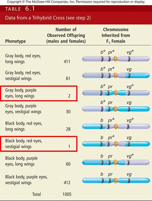
42 Step 3: Collect data for the F 2 generation 42

43 Analysis of the F 2 generation flies will allow us to map the three genes The three genes exist as two alleles each Therefore, there are 2 3 = 8 possible combinations of offspring If the genes assorted independently, all eight combinations would occur in equal proportions ( 즉, 1:1:1:1:1:1:1:1) It is obvious that they are far from equal In the offspring of crosses involving linked genes, Parental phenotypes occur most frequently Double crossover phenotypes occur least frequently Single crossover phenotypes occur with intermediate frequency Copyright The McGraw-Hill Companies, Inc. Permission required for reproduction or display 43

44 The combination of traits in the double crossover tells us which gene is in the middle A double crossover separates the gene in the middle from the other two genes at either end In the double crossover categories (F2 개체수가제일적은군 ), the recessive purple eye color is separated from the other two recessive alleles (Gray/purple/Long 또는 black/red/vestigial) Thus, the gene for eye color lies between the genes for body color and wing shape 44

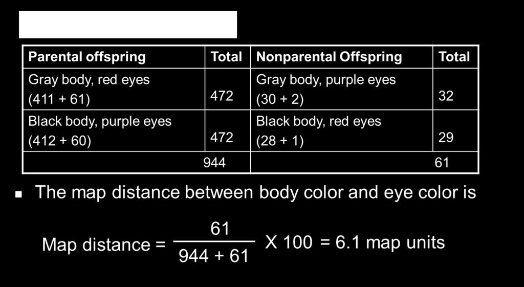
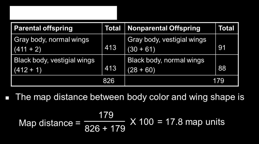
45 Step 4: Calculate the map distance between pairs of genes To do this, one strategy is to regroup the data according to pairs of genes From the parental generation, we know that the dominant alleles are linked, as are the recessive alleles This allows us to group pairs of genes into parental and nonparental combinations Parentals have a pair of dominant or a pair of recessive alleles Nonparentals have one dominant and one recessive allele The regrouped data will allow us to calculate the map distance between the two genes Copyright The McGraw-Hill Companies, Inc. Permission required for reproduction or display 45

46 46

47 Step 5: Construct the map Based on the map unit calculation the body color and wing shape genes are farthest apart The eye color gene is in the middle The data is also consistent with the map being drawn as vg pr b (from left to right) In detailed genetic maps, the locations of genes are mapped relative to the centromere Copyright The McGraw-Hill Companies, Inc. Permission required for reproduction or display 47

48 Interference The product rule allows us to predict the likelihood of a double crossover from the individual probabilities of each single crossover P (double crossover) = P (single crossover between b and pr) X P (single crossover between pr and vg) = X = Based on a total of 1,005 offspring The expected number of double crossover offspring is = 1,005 X = 7.5 Copyright The McGraw-Hill Companies, Inc. Permission required for reproduction or display 48

49 Interference Therefore, we would expect seven or eight offspring to be produced as a result of a double crossover However, the observed number was only three! Two with gray bodies, purple eyes, and normal sings One with black body, red eyes, and vestigial wings This lower-than-expected value is due to a common genetic phenomenon, termed positive interference The first crossover decreases the probability that a second crossover will occur nearby Copyright The McGraw-Hill Companies, Inc. Permission required for reproduction or display 49

50 Interference (I) is expressed as I = 1 C where C is the coefficient of coincidence C = Observed number of double crossovers Expected number of double crossovers C = = 0.40 I = 1 C = = 0.6 or 60% This means that 60% of the expected number of crossovers did not occur Copyright The McGraw-Hill Companies, Inc. Permission required for reproduction or display 50

51 Since I is positive, this interference is positive interference Rarely, the outcome of a testcross yields a negative value for interference This suggests that a first crossover enhances the rate of a second crossover The molecular mechanisms that cause interference are not completely understood However, most organisms regulate the number of crossovers so that very few occur per chromosome Copyright The McGraw-Hill Companies, Inc. Permission required for reproduction or display 51

52 6.4 GENETIC MAPPING IN HAPLOID EUKARYOTES Much of our earliest understanding of genetic recombination came from the genetic analyses of fungi Fungi may be unicellular or multicellular organisms They are typically haploid (1n) Haploid cells reproduce asexually Two haploid cells can fuse to form a diploid zygote (2n) which goes through meiosis to produce haploid spores The sac fungi (ascomycetes) have been particularly useful to geneticists because of their unique style of sexual reproduction Refer to Figure 6.11 Copyright The McGraw-Hill Companies, Inc. Permission required for reproduction or display 52

53 Figure

54 The cells of a tetrad or octad are contained within a sac In other words, the products of a single meiotic division are contained within one sac This is a key feature that dramatically differs from sexual reproduction in animals and plants In animals, for example Oogenesis only produces a single functional egg Spermatogenesis produces sperm that are mixed with millions of other sperm Using a microscope, researchers can dissect asci and study the traits of each haploid spore The analysis of these asci can be used to map genes Copyright The McGraw-Hill Companies, Inc. Permission required for reproduction or display 54

55 Types of Tetrads or Octads The arrangement of spores within an ascus varies from species to species Unordered tetrads or octads Ascus provides enough space for the spores to randomly mix together Ordered tetrads or octads Ascus is very tight, thereby preventing spores from randomly moving around Refer to Figure 6.12 Figure

56 Supplement Ordered Tetrad Analysis Ordered tetrads or octads have the following key feature The position and order of spores within the ascus is determined by the divisions of meiosis and mitosis This idea is schematically shown in Figure 6.S1 The example depicts ordered octad formation in Neurospora crassa Spores that carry the A allele show orange pigmentation Spores that carry the a (albino) allele are white Copyright The McGraw-Hill Companies, Inc. Permission required for reproduction or display 56

57 Supplement Figure 6.S1 57

58 Supplement The genetic content of spores in ordered tetrads can be determined This allows experimenters to map the distance between a single gene and the centromere The logic of this mapping technique is based on the following features of meiosis Centromeres of homologous chromosomes separate during meiosis I Centromeres of sister chromatids separate during meiosis II Refer to Figure 6.S2 Copyright The McGraw-Hill Companies, Inc. Permission required for reproduction or display 58

59 Supplement This 4:4 arrangement of spores within the ascus is termed a first-division segregation (FDS) or an M1 pattern Octad contains a linear arrangement of 4 haploid cells with the A allele which are adjacent to 4 with the a allele Because the A and a alleles have segregated from each other after meiosis I (a) First-division segregation (FDS) No crossing over produces a 4:4 arrangement. Figure 6.S2 (a) No crossing over Copyright The McGraw-Hill Companies, Inc. Permission required for reproduction or display 59

60 (b) Second-division segregation (SDS) A single crossover can produce a 2:2:2:2 or 2:4:2 arrangement. Supplement These arrangement of spores are termed a second-division segregation (SDS) or M2 patterns The A and a alleles do not segregate until meiosis II Figure 6.S2 (b) Single crossing over 60

61 Supplement Q: 왜 M2 asci 의퍼센트값은동원체와분석대상유전자간의거리를계산하는데만이용되는가? The percentage of M2 asci can be used to calculate the map distance between the centromere and the gene of interest -Crossover site 와 centromere 간의상호관계에대한이해가필요 The logic is that a gene is separated from its original centromere only after a crossover in the region between the gene and the centromere Figure 6.S3: The relationship between a crossover site and the separation of an allele from its original centromere 61

62 Supplement Therefore the chances of getting a 2:2:2:2 or 2:4:2 pattern depend on the distance between the gene of interest and the centromere To calculate this distance, the experimenter must count the number of SDS asci, as well as the total number of asci In SDS asci, only half of the spores are actually the product of a crossover (see Fig. 6-S2b) Therefore Map distance = (1/2) (Number of SDS asci) Total number of asci X 100 (spores 의개수를기준으로계산할수도있지만 asci 개수로하는것이편리함 ) Copyright The McGraw-Hill Companies, Inc. Permission required for reproduction or display 62

63 A numerical example of genetic mapping by ordered tetrad analysis (P generation: thr + arg + X thr arg) Supplement 63

64 Q1: Calculate the distance between the each gene and the centromere (1)The centromere thr distance -Draw an imaginary line via the middle of tetrads -Find groups with SDS pattern for thr : BDEG -Thus, percentage of SDS patterns = [(1/2)( )/105] X 100 = 10 m.u. (2) The centromere arg distance -Draw an imaginary line via the middle of tetrads -Find groups with SDS pattern for arg : CDEG -Thus, percentage of SDS patterns = [(1/2)( )/105] X 100 = 7.6 m.u. Supplement 64

65 Unordered Tetrad Analysis Unordered tetrads contain randomly arranged groups of spores An experimenter can do a dihybrid cross and then determine the phenotypes of the spores Such an analysis can determine if two genes are linked or assort independently It can also be used to compute distance between two linked genes Copyright The McGraw-Hill Companies, Inc. Permission required for reproduction or display 65

66 Unordered Tetrad Analysis Consider a diploid yeast zygote with the genotype ura + ura-2 arg + arg-3 ura + and arg + = Normal alleles required for uracil and arginine biosynthesis, respectively ura-2 and arg-3 = Defective alleles Result in strains that require uracil and arginine in their growth medium Figure 6.13 illustrates the assortment of the two genes in the unordered tetrad Copyright The McGraw-Hill Companies, Inc. Permission required for reproduction or display 66

67 Figure 6.13 PD Parental Ditype T Tetratype NPD Nonparental Ditype PD ascus: contains 100% parental cells T ascus: contains 50% parental cells and 50% recombinant cells NPD ascus: contains 100% recombinant cells 67

68 If the two genes assort independently The number of asci with a parental ditype is expected to equal the number with a nonparental ditype Thus, 50% recombinant spores are produced ( 멘델의유전법칙!) 68

69 If the two genes are linked The type of crossover between them determines what type of ascus is produced No crossovers yield the parental ditype Single crossovers produce the tetratype Double crossovers can yield any of the three types The actual type produced depends on the combination of chromatids that are involved Refer to Figure 6.14: crossing over 와 PD, NPD, T types 의생성과정의상호관계를알아보자 Copyright The McGraw-Hill Companies, Inc. Permission required for reproduction or display 69

70 Figure 6.14 No crossing over A single crossover Recombinant chromosomes Copyright The McGraw-Hill Companies, Inc. Permission required for reproduction or display 70

71 Figure 6.14c Double crossovers 71

72 As in conventional mapping, the map distance is calculated as the % of offspring that carry recombinant chromosomes Map distance = NPD + (1/2) (T) Total number of asci X 100 This calculation is fairly reliable over a short distance However, over long distances it is not Because it does not adequately account for double crossovers A more precise way to calculate map distance Map distance = Single crossover tetrads + (2) (Double crossover tetrads) Total number of asci Total number of crossovers X 0.5 X 100 Crossover tetrads also contain 50% nonrecombinant chromosomes (Why?) Copyright The McGraw-Hill Companies, Inc. Permission required for reproduction or display See Fig 6.14c 72

73 For the equation to be useful, it needs to be related to the number of various types obtained by experimentation So let s take another look at Figure 6.14 The parental ditype (PD) and tetratype (T) are ambiguous They can each be derived in two different ways (either single or double crossover) The nonparental ditype (NPD), however, is unambiguous It can only be produced from a double crossover (DCO) 1/4 of all the double crossovers are nonparental ditypes Therefore, DCO = 4 X NPD But what about single crossovers (SCO)? Notice that T asci can result from SCO or DCO T = SCO + DCO Since there are two kinds of T that are due to DCO The actual number of T arising from DCO is 2NPD So, T = SCO + 2NPD Therefore, SCO = T 2NPD 73

74 Now we have accurate measures of both SCO and DCO SCO = T 2NPD and DCO = 4NPD So, let s substitute these values into our previous equation Map distance = Single crossover tetrads + (2) (Double crossover tetrads) Total number of asci X 0.5 X 100 Map distance = (T 2NPD) + (2) (4NPD) Total number of asci X 0.5 X 100 Map distance = T + 6NPD Total number of asci X 0.5 X 100 A more accurate measure of map distance because the equation considers both single- and double-crossovers 74

75 A numerical example of genetic mapping by ordered tetrad analysis (P generation: thr + arg + X thr arg) PD types: AG NPD types: EF (3) T types: BCD (29) 75

76 Q2: Calculate the distance between the thr and arg The thr arg distance -To assure if the two genes are linked, we need to see if the tetrads in that group are PD, NPD, or T. -Ask PD >> NPD If so, they are linked. -Draw an imaginary line via the middle of tetrads -Find groups with PD or NPD or T -Thus, [{3+(1/2)( )}/105] X 100 = 16.7 m.u. (vs m.u. from the following equation) PD types: AG NPD types: EF (3) T types: BCD (29) 76

77 6.4 Mitotic Recombination Mitosis does not involve the homologous pairing of chromosomes to form bivalents Therefore crossing over in mitosis is expected to be much less likely than during meiosis Nevertheless, crossing over does occur on rare occasions In these cases, it may produce a pair of recombinant chromosomes that have a new combination of alleles This is known as mitotic recombination Crossing Over Occasionally Occurs During Mitosis 77

78 Stern was working with strains carrying X-linked genes affecting body color and bristle morphology y = yellow body color y + = gray body color sn = short body bristles (singed) sn + = normal body bristles Females that are y + y sn + sn are expected to have gray body and normal bristles However, when he microscopically observed these flies, he noticed places in which two adjacent regions were different from the rest of the body and from each other This is called a twin spot Stern proposed that twin spots are due to a single mitotic recombination within one cell during embryonic development Refer to Figure 6.15 Copyright The McGraw-Hill Companies, Inc. Permission required for reproduction or display 78

79 Figure

80 Figure

81 Chapter 07 Genetic transfer and mapping in bacteria and bacteriophages So far we focused on genetics of eukaryotes. Now we turn our attention to the genetic analysis of bacteria 81

82 INTRODUCTION Bacteria and viruses account for a quarter to a third of human deaths worldwide. Their impact on health is a major reason for studying them. Like eukaryotes, bacteria often possess allelic differences that affect their cellular traits However, these allelic differences (such as different sensitivity to antibiotics) are between different strains of bacteria because Bacteria are usually haploid This fact makes it easier to identify loss-of-function mutations in bacteria than in eukaryotes These usually recessive mutations are not masked by dominant genes in haploid species Bacteria reproduce asexually Therefore crosses are not used in the genetic analysis of bacterial species Rather, researchers rely on a similar phenomenon called genetic transfer In this process, a segment of bacterial DNA is transferred from one bacterium to another 82

83 7.1 GENETIC TRANSFER AND MAPPING IN BACTERIA Like sexual reproduction in eukaryotes, genetic transfer in bacteria enhances genetic diversity Transfer of genetic material from one bacterium to another can occur in three ways: Conjugation Involves direct physical contact Transduction Involves viruses Transformation Involves uptake from the environment See Table 7.1 Copyright The McGraw-Hill Companies, Inc. Permission required for reproduction or display 83

84 Table

85 Conjugation Genetic transfer in bacteria was discovered in 1946 by Joshua Lederberg and Edward Tatum They were studying strains of Escherichia coli that had different nutritional growth requirements Auxotrophs cannot synthesize a needed nutrient Prototrophs make all their nutrients from basic components One auxotroph strain was designated bio met phe + thr + It required one vitamin (biotin) and one amino acid (methionine) It could produce the amino acids phenylalanine and threonine The other strain was designated bio + met + phe thr Had the opposite requirements for growth Their experiment is described in Figure 7.1 Copyright The McGraw-Hill Companies, Inc. Permission required for reproduction or display 85

86 + : wild type functional gene copy - : mutant gene copy Figure 7.1: Experiment of Lederberg & Tatum demonstrating genetic transfer during conjugation 86

87 Bernard Davis later showed that the bacterial strains must make physical contact for transfer to occur using U-tube Figure 7.2 Thus, without physical contact, the two bacterial strains did not transfer genetic material to one another 87

88 The term conjugation now refers to the transfer of DNA from one bacterium to another following direct cell-to cell contact Many, but not all, species of bacteria can conjugate Moreover, only certain strains of a bacterium can act as donor cells Those strains contains a small circular piece of DNA termed the F factor (for Fertility factor) Strains containing the F factor are designated F + Those lacking it are F Plasmid is the general term used to describe extra-chromosomal DNA Figure

89 The first step in conjugation is the contact between donor and recipient cells This is mediated by sex pili (or F pili) which are made only by F + strains These pili act as attachment sites for the F bacteria Composed of pilin protein encoded by traa gene Refer to Figure 7.4b Once contact is made, the pili shorten Donor and recipient cell are drawn closer together A conjugation bridge is formed between the two cells This bridge provides a passageway for DNA transfer The successful contact stimulates the donor cells to begin the transfer process Refer to Figure 7.4a for the molecular details of conjugation Copyright The McGraw-Hill Companies, Inc. Permission required for reproduction or display 89

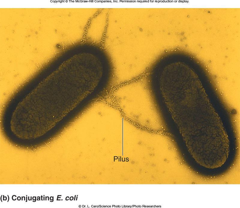
90 Cover image Fig

91 a complex of proteins encoded by the F factor that span both inner and outer membranes Together, these form the conjugation bridge Relaxosome recognizes a DNA sequence known as the origin of transfer. from its complementary strand Protein complex encoded by the F factor Accessory proteins of the relaxosome are released. One protein, relaxase, remains bound to the end of the T-DNA to form the complex called nucleoprotein between T DNA and relaxase Transferred DNA 2 nd step is the export of the nucleoprotein from donor to recipient. Figure 7.4a 91

92 Recipient receives single strand of the F factor DNA. Finally, the result of conjugation is that the recipient acquired an F factor, converting it from F- to F+ cell. Figure 7.4 Copyright The McGraw-Hill Companies, Inc. Permission required for reproduction or display 92

93 The result of conjugation is that the recipient cell has acquired an F factor Thus, it is converted from an F to an F + cell The F + cell remains unchanged In some cases, the F factor may carry genes that were once found on the bacterial chromosome These types of F factors are called F factors F factors can be transferred through conjugation This may introduce new genes into the recipient and thereby alter its genotype Copyright The McGraw-Hill Companies, Inc. Permission required for reproduction or display 93

94 Hfr Strains In the 1950s, Luca Cavalli-Sforza discovered a strain of E. coli that was very efficient at transferring chromosomal genes He designated this strain as Hfr (for High frequency of recombination) Hfr strains are derived from F + strains An episome is a segment of DNA that can exist as a plasmid and integrate into the chromosome Figure 7.5a Q: How to integrate into the host chromosome? See next slide. 94

95 F Plasmid Recombines into Genomic DNA by a single crossover 95 Figure Hyde genetics

96 In some cases, the integrated F factor is excised in an imprecise fashion may carry genes that were once found on the bacterial chromosome These types of F factors are called F factors F factors can be transferred through conjugation This may introduce new genes into the recipient cell and thereby alter its genotype William Hayes demonstrated that conjugation between an Hfr and an F strain involves the transfer of a portion of the Hfr bacterial chromosome The origin of transfer of the integrated F factor determines the starting point and direction of the transfer process One of the DNA strands is cut at the origin of transfer The cut, or nicked site is the starting point that will enter the F cell Then, a strand of Hfr bacterial DNA begins to enter into F- cell in a linear manner Copyright The McGraw-Hill Companies, Inc. Permission required for reproduction or display 96

97 It generally takes about hours for the entire Hfr chromosome to be passed into the F cell Most matings do not last that long Only a portion of the Hfr chromosome gets into the F cell Since the nick is internal to the integrated F factor, only part of the plasmid is transferred and the F cells does not become F + The F cell does pick up chromosomal DNA This DNA can recombine with the homologous region on the chromosome of the recipient cell via homologous recombination How does this process affect the recipient cell? This recombination may provide the recipient cell with new combination of alleles The recipient was originally lac - & pro -. Finally, F- cell becomes lac + & pro + depending on duration of mating time Refer to Figure 7.6 Copyright The McGraw-Hill Companies, Inc. Permission required for reproduction or display 97

98 lac + Ability to metabolize lactose lac Inability pro + Ability to synthesize proline pro Inability F cell received short segment of the Hfr chromosome It has become lac + but remains pro Copyright The McGraw-Hill Companies, Inc. Permission required for reproduction or display. pro + pro Hfr cell F cell Short time lac + lac + pro + lac + pro lac Transfer of Hfr chromosome pro + lac + pro lac Hfr cell F recipient cell lac + pro + Origin of transfer (toward lac + ) Therefore, the order of transfer is lac + pro + Figure 7.6 Longer time Has specific orientation and may be located in different regions of the chromosome. Thus the order of gene transfer depends on the location and orientation of the origin of transfer F cell received longer segment of the Hfr chromosome It has become lac + AND pro + How? Copyright The McGraw-Hill Companies, Inc. Permission required for reproduction or display pro + lac + pro + lac + 98

99 Crossover Events in Bacterial Transformation or conjugation Eukaryotes: A single co b/w two linear nonsister chromatids produces two recombinant linear chromatids Bacteria: A single co b/w a linear DNA molecule and the circular E. coli chromosome produces a recombinant linear DNA that cannot properly replicate Bacteria: A double co b/w a linear DNA molecule and the circular E. coli chromosome produces a circular recombinant DNA that can properly replicate Figure Hyde genetics 99

100 Hfr Transfer by bacterial conjugation (Hfr X F - matings) Figure

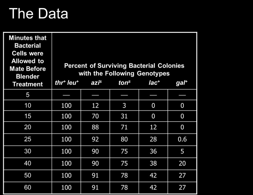
101 Experiment 7A: Interrupted Mating Technique At that time, not much information was known about the organization of bacterial genes along the chromosome Elie Wollman and F. Jacob realize that the process of gene transfer could be used to map the order of genes in E. coli This technique was developed by them in the 1950s The rationale behind this mapping strategy A blender treatment could be used to separate bacterial cells undergoing conjugation without killing them (called Interrupted mating) The time it takes genes to enter the recipient cell is directly related to their order along the bacterial chromosome The Hfr chromosome is transferred linearly to the F recipient cell Therefore, interrupted mating at different times would lead to various lengths being transferred The order of genes along the chromosome can be deduced by determining the genes transferred during short matings vs. those transferred during long matings 101

102 Wollman and Jacob started the experiment with two E. coli strains The donor (Hfr) strain had the following genetic composition thr + : Able to synthesize the essential amino acid threonine leu + : Able to synthesize the essential amino acid leucine azi s : Sensitive to killing by azide (a toxic chemical) ton s : Sensitive to infection by T1 (a bacterial virus) lac + : Able to metabolize lactose and use it for growth gal + : Able to metabolize galactose and use it for growth str s : Sensitive to killing by streptomycin (an antibiotic) The recipient (F ) strain had the opposite genotype thr leu azi r ton r lac gal str r r = resistant Copyright The McGraw-Hill Companies, Inc. Permission required for reproduction or display 102

103 Wollman and Jacob already knew that The thr + and leu + genes were transferred first, in that order Both were transferred within 5-10 minutes of mating Therefore their main goal was to determine the times at which genes azi s, ton s, lac +, and gal + were transferred The transfer of the str s was not examined Streptomycin was used to kill the donor (Hfr) cell following conjugation The recipient (F cell) is streptomycin resistant The Hypothesis The chromosome of the donor strain in an Hfr mating is transferred in a linear manner to the recipient strain The order of genes along the chromosome can be deduced by determining the time various genes take to enter the recipient cell Testing the Hypothesis (Figure 7.7) Copyright The McGraw-Hill Companies, Inc. Permission required for reproduction or display 103

104 Copyright The McGraw-Hill Companies, Inc. Permission required for reproduction or display. Experimental level Conceptual level 1. Mix together a large number of Hfr donor and F recipient cells. Hfr F Flask with bacteria lac + str s lac str r azi s azi r 2. After different periods of time, take a sample of cells and interrupt conjugation in a blender. lac + str s azi s lac str r azi r thr Separate by blending; donor DNA recombines with recipient cell chromosome. Figure Plate the cells on growth media lacking threonine and leucine but containing streptomycin. Note: The general methods for growing bacteria in a laboratory are described in the Appendix. 4. Pick each surviving colony, which would have to be thr + leu + str r, and test to see if It is sensitive to killing by azide, sensitive to infection by T1 bacteriophage, and able to metabolize lactose or galactose. Surviving colonies Bacterial growth Solid growth medium and streptomycin No growth +Azide +Lactose Overnight growth Sterile loop No growth Plaques +T1 phage +Galactose In this conceptual example, the cells have been incubated about 20 minutes. str s azi s Cannot survive on plates with streptomycin Additional tests str r Can survive on plates with streptomycin The conclusion is that the colony that was picked contained cells with a genotype of thr + leu + azi s ton s lac + gal str r. lac + azi s 104

105 105

106 Copyright The McGraw-Hill Companies, Inc. Permission required for reproduction or display 106

107 From these data, Wollman and Jacob constructed the following genetic map: They also identified various Hfr strains in which the origin of transfer had been integrated at different places in the chromosome (see next slides for details) Comparison of the order of genes among these strains, demonstrated the idea that the E. coli chromosome is circular Q: E.coli chromosome: circular or linear? Copyright The McGraw-Hill Companies, Inc. Permission required for reproduction or display 107

108 Hypothesis: Is the E.coli chromosome circular or linear? Linear: (1) azi lac gal (2) gal lac azi (3) lac azi (4) lac gal (5) azi gal lac (6) gal azi lac Circular: azi lac gal azi gal lac lac azi gal gal lac azi gal azi lac Note: 염색체가 Linear 인상태이면 Interrupted mapping 결과 gal azi 또는반대의순서로나올수없을것이다. 두유전자는연결되어있지않으므로! Q: 세균의염색체가 linear 상태라면 interrupted mating 실험결과나올수없는것에해당하는것은? 108

109 Supplement: Hyde genetics Mapping Genes by Time of Transfer during Conjugation 109

110 Supplement: Hyde genetics Generating a Map in E. Coli Using Information from Different Hfr Strains Figure Hyde genetics 110

111 Conjugation experiments have been used to map more than 1,000 genes on the E. coli chromosome The E. coli genetic map is 100 minutes long (Refer to Figure 7.8) Approximately the time it takes to transfer the complete chromosome in an Hfr mating The E. coli Chromosome Copyright The McGraw-Hill Companies, Inc. Permission required for reproduction or display 111

112 The distance between genes is determined by comparing their times of entry during an interrupted mating experiment The approximate time of entry is computed by extrapolating the time back to the origin Figure 7.9 Therefore these two genes are approximately 9 minutes apart along the E. coli chromosome Question From the Fig. 7.9, the lacz gene is located at 16 min on the chromosome map, and gale is found at 25 min. Deduce the location of the starting point (origin of transfer) on the chromosome map shown in Fig Note: The lacz gene is located at 7 min and the gale found at 16 min on the chromosome map 112

113 Supplement: Hyde genetics Mapping Genes in Conjugation by Recombination Stable expression of transferred alleles requires recombination into the E. coli chromosome Two crossover events required to recombine linear DNA into E. coli chromosome Order genes by looking at most and least frequent recombinants in recipient cell 113

114 Recombination mapping of linked genes after conjugation between Hfr Transferred Sequence and E. coli Chromosome Selection for this last gene Compare quadruple vs double crossovers : 가장표현형빈도가낮은종류가가장많은 crossovers 을통해생성된다. 따라서이종류에서세개유전자중가운데위치하는것을확인할수있음 (transfer time 만으로는서로매우가까운두유전자간의차이를구별할수없다 ) Figure

115 Transfer time of tyra and glya Supplement: Hyde genetics Figure min 차이 : interrupted mating 실험으로는구분하기어려움 115

116 An example of data analysis Supplement: Hyde genetics Hfr (str s, cysc +, tyra -, glya + ) X F- (str r, cysc -, tyra +, glya - ) We already know: cysc + allele was the last gene to enter Selection of str r, cysc + recombinants & replica plating str r, cysc +, tyra +, glya - : 30 str r, cysc +, tyra -, glya - : 2 str r, cysc +, tyra -, glya + : 78 str r, cysc +, tyra +, glya + : 0 (the quadruple crossover) tyra gene must be in the middle How to calculate the map distance between cysc and tyra : the percentage of all of the crossover events b/w two genes : (30/110)x(100%)=27.3 m.u. 116

117 Transduction is the transfer of DNA from one bacterium to another via a bacteriophage Transduction A bacteriophage is a virus that specifically attacks bacterial cells It is composed of genetic material surrounded by a protein coat It can undergo two types of life cycles Lytic : kill host Lysogenic: not harmful to host Figure Refer to Figure

118 Transduction Phages that can transfer bacterial DNA include P22, which infects Salmonella typhimurium P1, which infects Escherichia coli Both are temperate phages Figure 7.10 illustrates the process of transduction Figure

119 Transduction was discovered in 1952 by Joshua Lederberg and Norton Zinder They used an experimental strategy similar to that of Figure 7.1 They used two strains of the bacterium Salmonella typhimurium One strain, designated LA-22, was phe trp met + his + Unable to synthesize phenylalanine or tryptophan Able to synthesize methionine and histidine The other strain, designated LA-2, was phe + trp + met his Able to synthesize phenylalanine and tryptophan Unable to synthesize methionine or histidine Their experiment is described next Copyright The McGraw-Hill Companies, Inc. Permission required for reproduction or display 119

120 However, Lederberg and Zinder obtained novel results when repeating the experiment using the U-tube apparatus 120

121 Therefore, some agent was being transferred from LA-2 to LA-22 through the filter Norton and Zinder conducted the same experiment with filters of different pore sizes They found out that the filterable agent was less then 0.1mm in diameter They correctly concluded that the filterable agent was a bacteriophage In this case, the LA-2 strain contained a prophage (such as P22) The prophage switched to the lytic cycle Packaged a segment of DNA containing the phe + and trp + genes Passed through the filter and injected the DNA into the LA-22 strain Copyright The McGraw-Hill Companies, Inc. Permission required for reproduction or display 121

122 Cotransduction Mapping There is a maximum size to the DNA that can be packaged by bacteriophages during transduction P1 can pack up to 2-2.5% of the E. coli chromosome P22 can pack up to 1% of the S. typhimurium chromosome Cotransduction refers to the packaging and transfer of two closely-linked genes It is used to determine the order and distance between genes that lie fairly close together Copyright The McGraw-Hill Companies, Inc. Permission required for reproduction or display 122

123 Cotransduction Mapping (Two-factor transduction) Researchers select for the transduction of one gene They then monitor whether a second gene is cotransduced Consider for example the following two E. coli strains The donor strain with genotype arg + met + str s The recipient strain with genotype arg met str r The steps in a cotransduction experiment are presented in Figure 7.11 Figure

124 These colonies must be met + To determine whether they are also arg + streak onto plate that lacks both amino acids 21/50 124

125 (selection of met + ) Figure 7.11 met+ 인표현형의 colony 중 arg+ 인것의개수를확인해서테스트한전체 colony 수로나눈값이 cotransduction freq 임 이값은 met+ 와 arg+ 유전자가같이 transduction 될확률을의미함 125

126 T. T. Wu derived a relationship between cotransduction frequency and map distances obtained from conjugation experiments Cotransduction frequency = (1 d/l) 3 where Cotransduction Mapping d = distance between two genes in minutes L = the size of the transduced DNA (in minutes)» For P1 transduction, this size is ~ 2% of the E. coli chromosome, which equals about 2 minutes Let s use the equation in our example (arg + -met + ), Therefore, the distance between the met + and arg + genes is approximately 0.5 minutes Transduction experiments can provide very accurate mapping data for genes that are fairly close together Conjugation experiments, on the other hand, are usually used for genes that are far apart on the chromosome 126

127 Mapping with Cotransduction Supplement: Hyde genetics Three-factor transduction This method allows us to simultaneously establish gene order and relative distance ex: Infection of a - b - c - strain with a + b + c + phage Initial selection for first locus (selected locus) Replica plating for detecting other two loci Using the number of four classes transductants, calculate and compare cotransduction frequency of two genes Determine the rarest class(quadruple crossover) to identify the middle locus (see fig & 15.35) Higher percentage of cotransductants represents genes that are closer together 127

128 Mapping with Cotransduction Supplement: Hyde genetics 128

129 Mapping with Cotransduction Supplement: Hyde genetics Fig The rarest class: the middle gene is b - 129

130 Mapping with Cotransduction Supplement: Hyde genetics Figure

131 An example of data analysis How to calculate the cotransduction frequency of a+ and b+ : a+b+c+ (50) & a+b+c- (75), total (426) (100%)x(50+75)/426=29.3% Cotransduction freq. of a+ and c+: a+b+c+ (50) & a+b-c+ (1), total (426) (100%)x(50+1)/426=12.0% Supplement: Hyde genetics Gene order : a-b-c Relative distance: a-b 사이의거리는 a-c 보다가깝다 131

132 Distinguishing between mapping via conjugation and transduction Conjugation -Interrupted mapping 을통해 transfer time 을기준으로맨마지막으로전해진유전자에대한 recombinants 을선별함 ( 유전자들은 linear arrangement 로전달 ) -3 종류의유전자를가정할때나머지두개유전자는당연히 recipient cell 에전달되었을것이기때문에두유전자간의재조합빈도 (recombination frequency) 계산을통해 recombination distance 를추정하게됨 Supplement: Hyde genetics Cotransduction -Prototrophic bacteria 에 phage 를감염시킨후새로운 phage progeny 를확보해서 auxotrophic recipient cell 에감염시켜 3 개유전자중하나에대해선별한다 ( 이를통해무작위로절단된 DNA 조각이전달됨 ) -transduction 은도입순서는중요하지않고 recipient genome 으로함께 recombined 된두개유전자의 frequency 를계산한다 ( 전달된 DNA 조각에함께존재하는유전자만확인가능함 ) - 즉, 첫번째선별된유전자가 a + 이면 cotransduction frequency 는 a + -b + 또는 a + -c + 에대해계산한다. - 따라서 cotransduction frequency 가높아질수록두유전자의거리는가까운것임 132

133 Differences between conjugation and cotransduction mapping Box Figure 15a (hyde genetics chapter 15) 133

134 Let s now turn our attention to viruses Plaque formation and Intergenic complementation IN BACTERIOPHAGES Viruses are not living However, they have unique biological structures and functions, and therefore have traits We will focus our attention on bacteriophage T4 Its genetic material contains several dozen genes These genes encode a variety of proteins needed for the viral cycle : synthesis of new viruses (viral coat proteins) and lysis of the host cell Refer to Figure 7.13 for the T4 structure Figure

135 T4 phage as an experimental system T4 phage is DNA virus that can infect bacteria Can examine a large number of progeny to detect rare mutation events Could allow only recombinant phage to proliferate while parental phages died (can select only recombinant phage with combined genotype and altered traits) Plaques: one of phages traits A plaque is a clear area on an otherwise opaque bacterial lawn on the agar surface of a petri dish It is caused by the lysis of bacterial cells as a result of the growth and reproduction of phages The area of cell lysis creates a clear zone known as a viral plaque Figure

136 Working with T4 phage T4 phage (100,000X): Space ship! Life cycle of T4 phage Opaque lawn formed by uninfected bacterial cells A clear plaque containing millions of phages genetically identical (lysis of infected bacteria) 136

137 Some mutations in the phage s genetic material can alter the ability of the phage to produce plaques Thus, plaques can be viewed as traits of bacteriophages Plaques are visible with the naked eye So mutations affecting them lend (=provide) themselves to easier genetic analysis An example is a rapid-lysis mutant of bacteriophage T4, which forms unusually large plaques Refer to Figure 7.15 (Next slide) This mutant lyses bacterial cells more rapidly than do the wild-type phages Rapid-lysis mutant forms large, clearly defined plaques Wild-type phages produce smaller, fuzzy-edged plaques 137

138 Figure 7.15: Comparison of plaques produced by the wild-type T4 bacteriophage and a rapid-lysis mutant Figure

139 Benzer studied one category of T4 phage mutant, designated rii - (r stands for rapid lysis) He found phage yield in E. coli B was very low. He want to obtain large quantities of phages. So he tested other bacterial strains (E. coli K12S & K12 (λ)). Although wild-type phage could infect all three strains, rii - mutant behaved differently in three different strains of E. coli In E. coli B rii - phages produced unusually large plaques that had poor yields of bacteriophages The bacterium lyses so quickly that it does not have time to produce many new phages In E. coli K12S rii - phages produced normal plaques that gave good yields of phages In E. coli K12(l) (has phage lambda DNA integrated into its chromosome) Surprisingly, rii - phages were not able to produce plaques at all This lucky observation was critical feature that allowed intragenic mapping Copyright The McGraw-Hill Companies, Inc. Permission required for reproduction or display 139

140 Complementation Tests Can reveal if mutations are in the same gene or in different gene Benzer collected many rii mutant strains that can form large plaques in E. coli B and none in E. coli K12(l) (total 1612) Two genes (A and B) within rii locus are required for normal function For gene mapping, he needed to know if the mutations are in the same gene or in different genes? To answer this question, he conducted complementation experiments 140

141 Figure 7.16 shows the possible outcomes of complementation experiments involving plaque formation mutants Four different T4 phage strains (designated 1-4) carrying rii mutations were coinfected into E. coli K12(lamda) If two rii strains possess mutations in the same gene, noncomplementation occurs due to the absence of functional gene product A If the rii mutations are in different genes (such as gene A and gene B), a coinfected cell will have two mutant genes but also two wild type genes These cells can produce new phages and form plaques due to the presence of wild type copy of each gene The result is called complementation because the defective genes in each rii strain are complemented by the corresponding wild type genes Figure

142 Benzer carefully considered the pattern of complementation and noncomplementation He found out that the rii mutations occurred in two different genes, which were termed riia and riib This identification of two distinct genes affecting plaque formation was a key step for his intragenic mapping analysis Benzer coined (made) the term cistron to refer to the smallest genetic unit that gives a negative result of complementation test (noncomplementation) Since his studies, researchers have learned that a cistron is equivalent to a gene Although the term cistron is not popular at this time, the term polycistronic is still used to describe bacterial mrnas carrying two or more gene sequences So, if two mutations occur in the same cistron, they cannot complement each other Copyright The McGraw-Hill Companies, Inc. Permission required for reproduction or display 142

143 INTRAGENIC MAPPING IN BACTERIOPHAGES The study of viral genes provided insights into our basic understanding of how the genetic material works In the 1950s, Seymour Benzer embarked on a ten-year study focusing on the function of the T4 genes He conducted a detailed type of genetic mapping known as intragenic or fine structure mapping The difference between intragenic and intergenic mapping is: 143

144 Intragenic maps were conducted by analyzing recombination between mutants within the rii region At an extremely low rate, two noncomplementing strains of viruses can produce an occasional viral plaque, if intragenic recombination has occurred Figure

145 Figure 7.18 describes the general strategy for intragenic mapping of rii phage mutations Copyright The McGraw-Hill Companies, Inc. Permission required for reproduction or display 145

146 Take some of the phage preparation, dilute it greatly (10-8 ) and infect E. coli B Take some of the phage preparation, dilute it somewhat (10-6 ) and infect E. coli K12(l) (no infection by rii-) Both rii mutants and wild-type phages can infect this strain Phage E. coli K12(λ) rii mutants cannot infect this strain Total number of phages Number of wild-type phages produced by intragenic recombination 66 plaques 11 plaques 146