Human Genetics and Gene Mapping of Complex Traits
|
|
|
- Gabriella Davis
- 5 years ago
- Views:
Transcription
1 Human Genetics and Gene Mapping of Complex Traits Advanced Genetics, Spring 2018 Human Genetics Series Thursday 4/5/18 Nancy L. Saccone, Ph.D. Dept of Genetics /
2 What is different about Human Genetics (recall from Cristina Strong's lectures) Imprinting uniquely mammalian Trinucleotide repeat diseases "anticipation" Can study complex behaviors and cognition (neurogenetics) Extensive sequence variation leads to common/complex disease 1. Common disease, common variant hypothesis 2. Large # of small-effect variants 3. Large # of large-effect rare variants 4. Combo of genotypic, environmental, epigenetic interactions Greg Gibson, Nature Rev Genet 2012
3 Mapping disease genes Linkage quantify co-segregation of trait and genotype in families LOD score traditionally used to measure statistical evidence for linkage Association Common design: case-control sample, analyzed for allele frequency differences AC AC AC AA AC AA AC AA AC AA cases CC AC CC CC AC CC CC AC AA controls
4 Comparing Linkage and Association Linkage mapping: Requires family data Disease travels with marker allele within families (close genetic distance between disease locus and marker) Relationship between same allele and trait need not exist across the full sample (e.g. across different families) robust to allelic heterogeneity: if different mutations occur within the same gene/locus, the method works signals for complex traits tend to be broad (~20 Mb) Association mapping: Unrelated cases/controls OR Case/parents OR family design Disease is associated with marker allele that may be either causative or in linkage disequilibrium with causal variant Works only if association exists at the population level not robust to allelic heterogeneity association signals generally not as broad
5 Human DNA sequence variation Single nucleotide polymorphisms (SNPs) Strand 1: A A C C A T A T C... C G A T T... Strand 2: A A C C A T A T C... C A A T T... Strand 3: A A C C C T A T C... C G A T T... Provide biallelic markers Coding SNPs may directly affect protein products of genes Non-coding SNPs still may affect gene regulation or expression Low-error, high-throughput technology Common in genome
6 Number of SNPs in dbsnp over time solid: cumulative # of non-redundant SNPs. dotted: validated. dashed: double-hit from: The Intl HapMap Consortium Nature 2005, 437:
7 Number of SNPs in dbsnp over time dotted: validated From: Fernald et al., Bioinformatics challenges for personalized medicine, Bioinformatics 27:
8 Number of SNPs over time From: D. Koboldt s blog, Sept (
9 Questions that we can answer with SNPs: Which genetic loci influence risk for common human diseases/traits? (Disease gene mapping studies, including GWAS genome-wide association studies) Which genetic loci influence efficacy/safety of drug therapies? (Pharmacogenetics) Population genetics questions evidence of selection identification of recombination hotspots
10 Part I: Human linkage studies Need to track co-segregation of trait and markers (number of recombination events among observed meioses) General linkage screen" approach: Recruit families Genotype individuals at marker loci along the genome If a marker locus is "near" the trait-influencing locus, the parental alleles from the same grandparent at these two loci "tend to be inherited together" (recombination between the two loci is rare) = the probability of recombination between 2 given loci Defn: max LOD score = ˆ log 10 [ L( ˆ) / L( 1/ 2)] ( is the maximum likelihood estimate of theta)
11 Example of autosomal dominant (fully penetrant, no phenocopies) General hallmarks: All affected have at least one affected parent, so the disease occurs in all generations above the latest observed case. The disease does not appear in descendants of two unaffecteds. Possible molecular explanation: disease allele codes for a functioning protein that causes harm/dysfunction. Figure from Strachan and Read, Human Molecular Genetics
12 Example of autosomal recessive (fully penetrant, no phenocopies). General hallmarks: Many/most affecteds have two unaffected parents, so the disease appears to skip generations. On average, 1/4 of (carrier x carrier) offspring are affected. (Affected x unaffected) offspring are usually unaffected (but carriers) (Affected x affected) offspring are all affected. Figure from Strachan and Read, Human Molecular Genetics
13 Figure from Strachan and Read, Human Molecular Genetics Example of autosomal recessive (fully penetrant, no phenocopies). Possible molecular explanation: disease allele codes for a nonfunctional protein or lack of a protein, and one copy of the wild-type allele produces enough protein for normal function.
14 Classic models of disease Classical autosomal dominant inheritance (no phenocopies, fully penetrant). Penetrance table: f ++ f +d f dd Often the dominant allele is rare, so that probability of homozygous dd individuals occurring is negligible. Classical autosomal recessive inheritance (no phenocopies, fully penetrant). Penetrance table: f ++ f +d f dd 0 0 1
15 Genetic models of disease Other examples of penetrance tables (locus-specific): f ++ f +d f dd Incomplete/reduced penetrance: when the risk genotype's effect on phenotype is not always expressed/observed. (e.g. due to environmental interaction, modifier genes) Phenocopy: individual who develops the disease/phenotype in the absence of "the" risk genotype (e.g. through environmental effects, heterogeneity of genetic effects)
16 Part II: Genetic Association Testing Typical statistical analysis models: Quantitative continuous trait: linear regression Dichotomous trait e.g. case/control: logistic regression - more flexible than chi-square / Fisher s exact test - can include covariates - provides estimate of odds ratio
17 Let y = quantitative trait value ŷ OR ŷ = + b Linear regression y = + b1x1 b2x2... bnx 1x1 b2x2... bnxn predicted quantitative trait value error x 1 = SNP genotype (e.g. # copies of designated allele: 0,1,2) x 2,, x n are covariate values (e.g. age, sex) n a.k.a. residual Null hypothesis H 0 : b 1 = 0. The SNP effect size is represented by b 1, the coefficient of x 1. Is there significant evidence that b 1 is non-zero?
18 Least squares linear regression: general example y = + b x y Fitted line, Slope = b Residual deviations x The least squares solution finds and b that minimize the sum of the squared residuals.
19 Least squares linear regression: general example y = + b x y Fitted line, Slope = b Residual deviations Would NOT minimize the sum of squared residuals x The least squares solution finds and b that minimize the sum of the squared residuals.
20 SNP Marker Additive Coding: Genotype x 1 1/1 0 1/2 1 2/2 2 Codes number of 2 alleles
21 y = + b x Least squares linear regression b = slope of Fitted line x-axis: number of alleles
22 y = + b x Phenotypic variance explained b = slope of Fitted line x-axis: number of alleles r 2 = squared correlation coefficient Indicates proportion of phenotypic variance in y that s explained by x
23 Another use of linear regression: Traditional sib pair linkage analysis Model-free / non-parametric Idea: if two sibs are alike in phenotype, they should be alike in genotype near a trait-influencing locus. to measure "alike in genotype" : Identity by descent (IBD). Not the same as identity by state IBS=1 IBD=0 IBS=1 IBD=1
24 Sib pair linkage analysis of quantitative traits Haseman-Elston regression: Compare IBD sharing to the squared trait difference of each sib pair. (trait difference) IBD
25 Example sib-pair based LOD score plot., from Saccone et al., 2000
26 Logistic regression for dichotomous traits Let y = 1 if case, 0 if control (2 values) Let P = probability that y = 1 (case) Let x 1 = genotype (additive coding) Why? logit(p) ln P 1- P = + b 1x1 b2x 2... bnx n
27 Logit function Usual regression expects a dependent variable that can take on any value, (-,) A probability is in [0,1], so not a good dependent variable Odds = p/(1-p) is in [0,) Logit = ln(odds) is in (-,)
28 Think of the shapes of the graphs y = x/(1-x) (x in place of P) As x varies from 0 to 1, y varies from 0 to 1 y=ln(x) varies from - to
29 Logistic regression Let y = 1 if case, 0 if control (2 values) Let P = probability that y = 1 (case) logit(p) ln P 1- P = + b 1x1 b2x 2... bnx n Note that can exponentiate both sides to get odds = P / (1-P): Odds P 1- P = e + b1x1b2x 2... bnx n e What about the effect size? It s the odds ratio, and it is still related to b 1!
30 Odds ratio The number e (=2.718 ) is the base of natural logarithms e 0 1 e b 1 is the odds ratio; if b 1 =0 then odds ratio is 1
31 To get odds ratio per copy of the allele ( effect size ) Full model: Odds when x 1 = 1 (1 copy of the allele) Odds when x 1 = 0 (0 copies of the allele) Odds Ratio: ]... [ nx n x e P P b b ]... [ 0 ]... [ ) 1 /( n n n n x x x x x e e P P b b b b ]... [ 1 ]... [ 1 1 ) /(1 b b b b b n n n n x x x x x e e P P 1 n n n n 2 2 ] x... x + [ ] x... x + [ = 1 1 b b b b b b e e e ) P /( P P ) P /(
32 Logistic regression summary Let y = 1 if case, 0 if control (2 values) Let P = probability that y = 1 (case), ranges from 0 to 1 Then logit(p) ranges from - to logit(p) ln P 1- P = + b 1x1 b2x 2... bnx n Odds ratio e b 1 Similar to case of linear regression, can compute an analog to variance explained, usually also called r 2
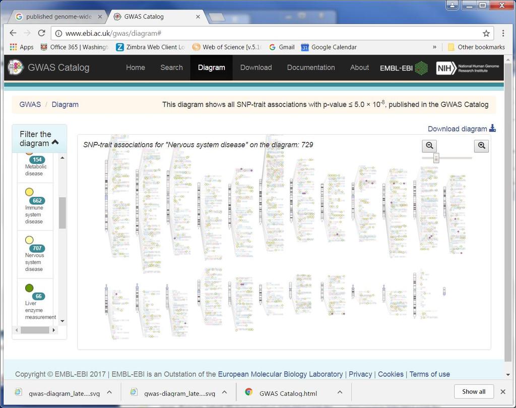
 http://www.ebi.ac.")
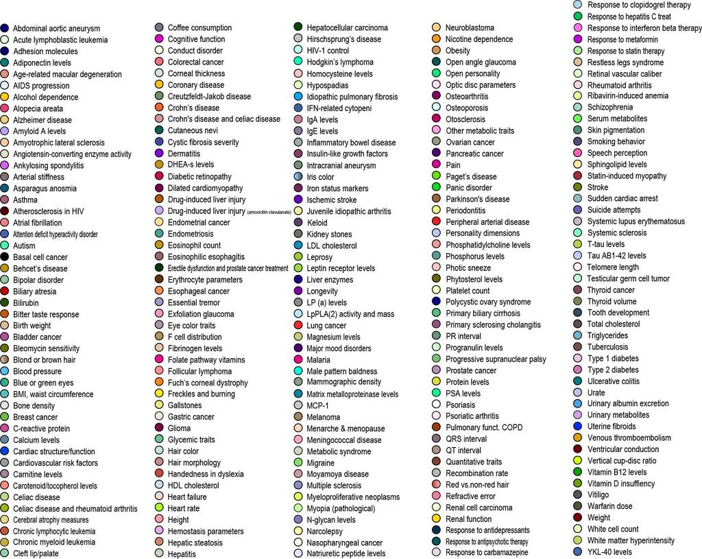
33 Published Genome-Wide Associations (p 5x10⁻⁸ )
34
35
36 Displaying GWAS results Manhattan plot x-axis: chromosomal position y-axis: -log 10 (p-value) p = 1x10⁻⁸ is plotted at y=8, p = 5x10⁻⁸ is plotted at y = 7.3 Q-Q plot Quantile-Quantile plot Idea: Rank tested SNPs by association evidence; compare number of observed vs expected associations under the null at a given significance level Bloom et al., Ann Am Thorac Soc 2014
37 Displaying GWAS results Q-Q plot : Quantile-quantile plot Idea: Rank tested SNPs by association evidence; compare number of observed vs expected associations under the null at a given significance level Helps detect systematic bias in data: Most datapoints should be close to the y=x line Exception: signals (lowest, most significant p-values)
38 Displaying GWAS results Q-Q plot : Quantile-quantile plot JAMA 299: (2008)
39 Successful by several metrics: GWAS Identifying genetic variants underlying complex diseases Highlighting novel genes, pathways, biology Motivating functional followup, collaborative meta-analyses Less successful by other metrics: "Top" associated SNPs explain limited phenotypic variance (typical odds ratios ~ 1.3, variance explained ~ 1%) But even by that metric, there's good news: As a whole, the variation assayed by GWAS may be able to explain even more of the phenotypic variance (work of Peter Visscher et al.) GWASes rely on linkage disequilibrium (LD) to "tag" variation, and thus must be interpreted in the context of LD: the signal SNP may be different from the causal SNP.
40 Interpretation of GWAS results must account for LD Suppose a SNP is significantly associated with a disease Other SNPs correlated (high r 2 ) with that SNP are additional, potentially causative variants Example: CHRNA5-CHRNA3-CHRNB4 on chromosome 15q25 Nicotinic receptor gene cluster CHRNA5-CHRNA3-CHRNB4 rs D398N in CHRNA5 Saccone SF et al., 2007
41 Example: CHRNA5-CHRNA3-CHRNB4 and rs Associated with nicotine dependence, smoking, lung cancer, COPD. CHRNA5-CHRNA3-CHRNB4 Hap Map CEU r Also others rs Hung et al., 2008 Amos et al., 2008 Pillai et al., 2009 rs Saccone SF et al., 2007 Bierut et al., 2008 Stevens et al., 2008 Sherva et al., 2008 Chen et al., 2009 Weiss et al., 2009 Liu et al, 2008 Young et al., 2008 rs Berrettini et al., 2008 rs Saccone SF et al., 2007 Thorgeirsson et al., 2008 Caporaso et al., 2009 Hung et al., 2008 Amos et al., 2008 Pillai et al., 2009
42 ancestral chromosome present day chromosomes: LD and Human Sequence Variation alleles on the preserved "ancestral background" tend to be in linkage disequilibrium (LD)
43 Linkage Disequilibrium Potential sources of LD : 1. Genetic linkage between loci 2. Random drift 3. Founder effect 4. Mutation 5. Selection 6. Population admixture / stratification
44 Linkage Disequilibrium (LD) involves haplotype frequencies. Focus on pair-wise LD, SNP markers Genotypes do not necessarily determine haplotypes: Consider 2-locus genotype A 1 A 2 B 1 B 2. Two possible phases :
45 Linkage Disequilibrium (LD) involves haplotype frequencies Focus on pair-wise LD, SNP markers Genotypes do not necessarily determine haplotypes: Consider 2-locus genotype A 1 A 2 B 1 B 2. Two possible phases : A 1 A 2 A 1 A 2 B 1 B 2 B 2 B 1
46 Linkage Disequilibrium Linkage Disequilibrium (LD), aka allelic association: For two loci A and B: LD is said to exist when alleles at A and B tend to cooccur on haplotypes in proportions different than would be expected under statistical independence.
47 Linkage Disequilibrium Example: Consider 2 SNPs: SNP 1: A 50% C 50% SNP 2: A 50% G 50% snp1 snp2 expected freq 4 possible haplotypes: A A 0.5 * 0.5 A G 0.5 * 0.5 C A 0.5 * 0.5 C G 0.5 * 0.5 But perhaps in your sample you observe only the following: A A C C A T A T C... C G A T T... and A A C C C T A T C... C A A T T...
48 Linkage Disequilibrium How to formally measure LD between alleles at 2 loci?
49 To measure LD between alleles at 2 biallelic loci Locus A Locus B B 1 B 2 A 1, A 2 B 1, B 2 Given 2N haplotypes: Haplotype freq for A i B j is A 1 A 2 n11 n21 n12 n22 Compare h ij to the frequency expected under no association: 2N Define the disequilibrium coefficient:
50 Disequilibrium coefficient: Common LD measures D = h 11 - p A 1 p B1 Normalized disequilibrium coefficient: D' = D / D max, where Range of D' is [-1,1] Squared correlation coefficient: r 2 = D 2 / ( p A 1 p A2 p B1 p B2 )
51 Measuring LD Example: B 1 B 2 B 1 B 2 Only observe 2 haplotypes: A 1 B 1 and A 2 B 2 A A A 2 A observed expected D = h 11 p A1 p B1 = (0.5) (0.5)(0.5) = = 0.25 D max = min(p A1 p B2, p A2 p B1 ) = min(0.25,0.25) = 0.25 D' = 1, r 2 = 1
52 Measuring LD Example: B 1 B 2 B 1 B 2 Only observe 2 haplotypes: A 1 B 1 and A 2 B 2 A A A 2 A observed expected To measure significance: c 2 (1 df): Chi-sqr = 100, r 2 = 1, D' = 1