Dan Geiger. Many slides were prepared by Ma ayan Fishelson, some are due to Nir Friedman, and some are mine. I have slightly edited many slides.

Transcription

1 Dan Geiger Many slides were prepared by Ma ayan Fishelson, some are due to Nir Friedman, and some are mine. I have slightly edited many slides.

2 Genetic Linkage Analysis A statistical method that is used to associate functionality of disease genes to their approximate location on the chromosome using pedigree data of affected families. Main idea: genes and markers that reside in vicinity on the chromosome have a tendency to stick together when passed on to offsprings. Some disease is often passed to offsprings along with specific markers the gene responsible for the disease is located close on the chromosome to these markers. 2

3 Outline Part I: Reminder about genetics Part II: mathematics/algorithms Part III: Software description Part IV: Software demonstration online (by Gideon Greenspan) 3

4 Genetic Information Gene basic unit of genetic information. They determine the inherited characters. Genome the collection of genetic information. Chromosomes storage units of genes. 4

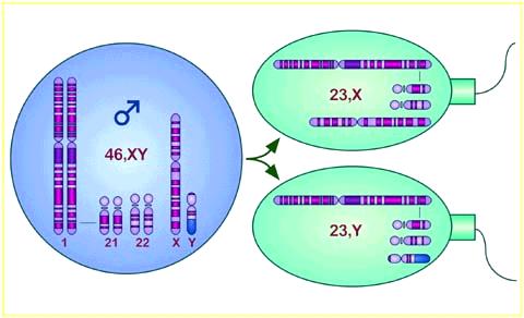
5 Human Genome Most human cells contain 46 chromosomes: 2 sex chromosomes (X,Y): XY in males. XX in females. 22 pairs of chromosomes named autosomes. 5

6 Chromosome Structure Locus the location of genes on the chromosome. Allele one variant form (or state) of a gene at a particular locus. Locus1 Possible Alleles: A1,A2 Locus2 Possible Alleles: B1,B2,B3 6

7 Alleles genotype phenotype E b - dominant allele. E w - recessive allele. 7

8 Genotypes versus Phenotypes At each locus (except for sex chromosomes) there are 2 genes. These constitute the individual s genotype at the locus. The expression of a genotype is termed a phenotype. For example, hair color, weight, or the presence or absence of a disease. Also measured unordered pairs of genes are now considered phenotype (at least mathematically). 8

9 Sexual Reproduction egg sperm zygote gametes 9

10 Recombination Phenomenon I. The exchange of pieces of homologous chromosomes during formation of gametes. II. A recombination between 2 genes occurred if the haplotype of the individual contains 2 alleles that resided in different haplotypes in the individual's parent. (Haplotype the alleles at different loci that are received by an individual from one parent). 10

11 Two Loci Inheritance A A B B 1 2 a a b b A a B b 3 4 a a b b Recombinant 5 A a b b 6 A a B b 11

12 An example - the ABO locus. The ABO locus determines detectable antigens on the surface of red blood cells. The 3 major alleles (A,B,O) interact to determine the various ABO blood types. O is recessive to A and B. Alleles A and B are codominant. Phenotype A B AB O Genotype A/A, A/O B/B, B/O A/B O/O Note that the listed genotypes are unordered (we don t know which allele is from the father and which one is from the mother). 12

13 Example: ABO, AK1 on Chromosome 9 A A 1 /A O A 2 /A 2 O O A 2 A 2 A A A O 3 4 A O A 1 A 2 A 1 /A 2 A 2 /A 2 A 2 A 2 Recombinant O O A 1 A 2 O A 1 /A 2 5 Male recombination fraction 0.12 and female

14 Comments about the example Often: Pedigrees are larger and more complex. Not every individual is typed. Recombinants cannot always be determined for certain. There are more markers and they are polymorphic (not di-allelic). 14

15 Part II: Relevant Mathematics 15

16 Probabilistic model for inheritance I Each node represents a random variable that has a finite number of states. The states for L 11m, L 11f, L 13m are the possible alleles at locus 1. The states of X 11 are the possible unordered allele-pairs at locus 1. The states of S 13m are 0 or 1 depending whose allele is transmitted to the offspring. Each node is associated with a conditional probability table. 16

17 Probabilistic model for inheritance II 17

18 Probabilistic model for inheritance III 18

19 19

20 Probabilistic model for Recombination P( s 23t s 13t ) 1 θ = θ 2 2 θ 2 1 θ 2 where t {m,f} θ 20

21 Recombination Fraction The recombination fraction between two loci is a monotone, nonlinear function of the physical distance separating between the loci. It is measured in terms of centi-morgans. One centimorgan means one recombination every 100 meiosis. Recombination fraction can change between males and females. So in the previous slide we might want to have: P( s 23m s 13m 1 θ ) = θ 2m 2m θ 2m 1 θ 2m P( s 23 f s 13 f 1 θ ) = θ2 f 2 f θ 2 f 1 θ 2 f ( Linkage) 0 < θ P(Recombination) 0.5 (No Linkage) 21

22 Having a disease Locus P( s 23t s 13t' ) = 1 θ θ 2 2 θ 2 1 θ 2 θ 22

23 Maximum Likelihood Approach θ θ θ θ 23

24 24 Generalization: Bayesian Network Bayesian network = Directed Acyclic Graph (DAG), annotated with conditional probability distributions. ), ( ) ( ), ( ) ( ) ( ) ( ) ( ) ( ),,,,,,, ( b a d P a x P l t a P s b P s l P v t P s P v P d x a b l t s v P = p(t v) p(x a) p(d a,b) p(a t,l) p(b s) p(l s) p(s) p(v)

25 The Visit-to-Asia Example 25

26 Local distributions p(a T,L) Table: p(a=y L=n, T=n) = 0.02 p(a=y L=n, T=y) = 0.60 p(a=y L=y, T=n) = 0.99 p(a=y L=y, T=y) =

27 Exact Inference: Variable Elimination General idea: Write a query in the form P( data) = L x x x k k m 3 1 i= 1 P( x i pa i ) Iteratively Move all irrelevant terms outside of innermost sum Perform innermost sum, getting a new term Insert the new term into the product 27

28 We want to compute Need to eliminate: Initial factors 28

29 We want to compute Need to eliminate: Initial factors Eliminate: Compute: = Note: In general, as we will see, the result of elimination is not necessarily a probability distribution. 29

30 We want to compute Need to eliminate: Initial factors Eliminate: Compute: = Summing on results in a factor with two arguments In general, the result of elimination may be a function of several variables. 30

31 We want to compute Need to eliminate: Initial factors Eliminate: Compute: = Note: for all values of 31

32 We want to compute Need to eliminate: Initial factors Eliminate: Compute: = 32

33 We want to compute Need to eliminate: Initial factors Eliminate: Compute: = 33

34 We want to compute Need to eliminate: a, Initial factors Eliminate: Compute: = = 34

35 Comments on Variable Elimination Actual computation is done in the elimination step. Computation depends on the order of elimination as in computing products of matrices. 35

36 Summation order in GeneHunter 36

37 GeneHunter summation order defines a Hidden Markov Model (HMM) 37

38 Hidden Markov Model (HMM) 38

39 Part III: Software for Genetic Analysis Fastlink v4.1 (Our students have contributed) Vitesse v1, v2 GeneHunter Scores of other packages SuperLink (Temporary name, being developed here) See 39

40 Existing Programs for Genetic Linkage Analysis 40

41 The future: SUPERLINK Stage 1: each pedigree is translated into a Bayesian network. Stage 2: value elimination is performed on each pedigree (i.e., some of the impossible values of the variables of the network are eliminated). Stage 3: an elimination order for the variables is determined, according to some heuristic. Stage 4: the likelihood of the pedigrees given the theta values is calculated. This is done by by performing variable elimination according to the elimination order determined in stage 3. 41

42 Special Features 42

43 Value Elimination & Allele Exclusion A preprocessing step that reduces the range of feasible values for the variables of the Bayesian network given the data. Results in major savings in the time and memory requirements of the likelihood calculations. 43

44 Time-Space Tradeoff For many data sets, the use of variable elimination alone isn t enough, due to the large memory overhead. Superlink combines variable elimination with conditioning to achieve the best time-space tradeoff given the available memory. Conditioning is performed only after some steps of variable elimination, when the memory requirements are about to exceed the limitations. 44

45 Probability Table Representation All probability tables are defined in a flexible size which depends on viable variable combinations. Each table is represented by a onedimensional array of double-precision numbers. In addition, the number of possible values for each variable is stored. A special indexing method allows for quick access to the entrances of the table. 45

46 Experiment A Same topology (57 people, no loops) Increasing number of loci (each one with 4-5 alleles) Run time is in seconds. Files No. of Run Time Run Time Run Time Run Time Loci Superlink Fastlink Vitesse Genehunter A A A A A A A A A A A A11 40 over 100 hours Out-of-memory Pedigree size Too big for Genehunter. 46

47 Experiment B Same topology (100 people, with loops) Increasing number of loci (each one with 5-10 alleles) Run time is in seconds. Files No. of Run Time Run Time Run Time Run Time Loci Superlink Fastlink Vitesse Genehunter B B B B B B B B B B B B Out-of-memory Vitesse doesn t handle looped Pedigrees. Pedigree size Too big for Genehunter. 47

48 Experiment C Same topology (5 people, no loops) Increasing number of loci (each one with 3-6 alleles) Run time is in seconds. Files No. of Run Time Run Time Run Time Run Time Loci Superlink Fastlink Vitesse Genehunter D (2 l.e.) 0.41 (99 l.e.) D (2 l.e.) 0.45 (109 l.e.) D (2 l.e.) 0.48 (119 l.e.) D (2 l.e.) 0.49 (129 l.e.) D (2 l.e.) 0.51 (139 l.e.) D (2 l.e.) 0.53 (149 l.e.) D (2 l.e.) 0.54 (159 l.e.) D (2 l.e.) 0.6 (169 l.e.) D (2 l.e.) 0.59 (179 l.e.) D (2 l.e.) 0.61 (189 l.e.) D (2 l.e.) 0.66 (199 l.e) D (2 l.e.) 0.67 (209 l.e) Bus error Out-of-memory 48

49 Partial References Kenneth Lange Mathematical and Statistical Methods for Genetic Analysis Jurg Ott Analysis of Human Genetic Linkage