Monday, November 8 Shantz 242 E (the usual place) 5:00-7:00 PM

Transcription

1 Review Session Monday, November 8 Shantz 242 E (the usual place) 5:00-7:00 PM I ll answer questions on my material, then Chad will answer questions on his material.

2 Test Information Today s notes, the review questions and a separate list of study questions will be posted on the website tomorrow (Friday). If you re just dying to have them this afternoon, send me an and I ll send them to you. I will be down in the lab (Forbes 113) this morning during office hours. I can answer questions, but it may take a few minutes for me to get to you.

3 Quantitative Genetics

4 Polygenic Inheritance In previous lectures, we ve examined traits in which the phenotypic variation can be distinctly classified (offspring either like a parent or intermediate between the two). This is referred to as discontinuous variation. continuous Many other traits demonstrate continuous variation, and are characterized by a range of phenotypes in the offspring.

5 Polygenic Inheritance You should note that polygenic inheritance can only be studied in populations because there are multiple genes and multiple alleles being studied. Two individuals cannot account for all the alleles controlling the phenotype. In order to assess the influence of all the alleles available, multiple individuals must be studied to observe all the phenotypes resulting from the different genotypes.

6 Polygenic Inheritance Traits exhibiting continuous variation are usually controlled by two or more genes. All of the genes influencing the phenotype have an additive effect on the phenotype: each gene adds to the phenotype. This effect can be quantified.

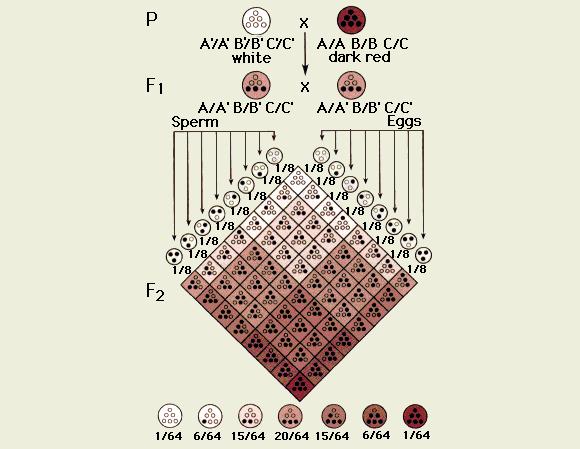
7 Polygenic Inheritance An example: wheat berry color. Cross true-breeding plants with white berries to truebreeding plants with dark red berries. The resulting F 1 all exhibit an intermediate color. When the F 1 s are crossed, the result is a range of color.

8

9 This is called a bell curve, and demonstrates a normal distribution

10 Polygenic Inheritance When individual plants from the F2 are selected and mated, the phenotype of the resulting offspring also produces a range of phenotypes and a similarly shaped curve: There is a range of phenotypes, but most of the offspring are similar in color to the parents.

11 Early Experiments The fact that offspring of later crosses could be segregated into distinct phenotypic classes allowed researchers to propose that multiple factors were responsible for the phenotypes, and that these factors all contributed to the appearance.

12 The Basis of Additive Inheritance 1. Characteristics can be quantified (measured, counted, weighed, etc.) 2. Two or more genes, at different places in the genome, influence the phenotype in an additive way (polygenic). 3. Each locus may be occupied by an additive allele that does contribute to the phenotype, or a nonadditive allele, which does not contribute.

13 The Basis of Additive Inheritance 4. The total effect of each allele on the phenotype, while small, is roughly equal to the effects of other additive alleles at other gene sites. 5. Together, the genes controlling a single character produce substantial variation in phenotype. 6. Analysis of polygenic traits requires the study of large numbers of progeny from a population of organisms.

14 Back to the First Example

15 Determining the Number of Genes The number of genes may be calculated if --the proportion of F2 individuals expressing either of the two most extreme (i.e. parental) phenotypes can be determined according to the following formula: 1/4 n =proportion of offspring either red or white

16 Determining the Number of Genes In our previous example, 1/64 of the F2 wheat berries were either red or white. 1 = 1 4 n 64 Then, solve for n, which in this case, is 3.

17 Another Method to Determine the Number of Genes: The (2n + 1) Rule If n = the number of gene pairs, then (2n + 1) will determine the total number of categories of phenotypes. In our example, there were 7 phenotype classes: (2n + 1) = 7 (7-1) = 6 = 3 2 2

18 Significance of Polygenic Control Most traits in animal breeding and agriculture are under polygenic control: Height, weight, stature, muscle composition, milk and egg production, speed, etc.

19 Genotype Plus Environment Note that genotype (fixed at fertilization) establishes the range in which a phenotype may fall, but environment influences how much genetic potential will be realized. (So far, we have assumed no influence of environment on the cross examples used)

20 Biometry Biometry is the quantitative study of biology and utilizes statistical inference to analyze traits exhibiting continuous variation. While the observations of an experiment are hoped to represent the population at large, there may be random influences affecting samples that adds to variation in the study population. Statistical analysis allows researchers to predict the sources of variation and the relative influence of each source.

21 Purposes of Statistical Analysis 1. Data can be analyzed mathematically and reduced to a summary description. 2. Data from a small but representative and random sample can be used to infer information about groups larger than the study population (statistical inference). 3. Two or more sets of experimental data can be compared to determine if they represent different populations of measurements.

22 Mean: The distribution of two sets of phenotypic measurements cluster around a central value. The mean is the arithmetic average of the set of measurements, the sum of all of the individuals divided by the number of individuals. Statistical Terms

23 Mean The mean is arithmetically calculated as Mean = X i /n Where X i is the sum of all the individual values and n is the number of individual values

24 Mean Observed values for eight samples {2,2,4,4,5,6,6,8} X i is 38 38/8 = 4.75 Therefore, the mean for this sample is 4.75

25 Median If the data are arranged from smallest to largest value, the median value is the central number. {2,2,4,4,5,6,6,7,8} So the median value for this data set is 5.

26 Range Range is the distance between the smallest value in a set and the largest value in a set. {2,2,4,4,5,6,6,7,8} The range for this set is 2 to 8.

27 Frequency Distribution Median and range give information about the frequency distribution, or shape of the curve. The values of two different data sets may have the same mean, but be distributed around that mean differently.

28 Variance Variance is a value that describes the degree to which the values in a data set diverge from the mean. The variance within the data set is used to make inferences or estimate the variation in the population as a whole.

29 Calculate Variance (s 2 ) s 2 = (X i -mean) 2 /n -1