Long-term dynamics of CA1 hippocampal place codes

Transcription

1 Long-term dynamics of CA1 hippocampal place codes Yaniv Ziv, Laurie D. Burns, Eric D. Cocker, Elizabeth O. Hamel, Kunal K. Ghosh, Lacey J. Kitch, Abbas El Gamal, and Mark J. Schnitzer Supplementary Fig. 1 Ca 2+ dynamics of CA1 pyramidal cells visualized during active mouse behavior. (a, b) We extracted the spatial locations, (a) (perimeters encircled in color), and time traces of Ca 2+ activity of 289 CA1 pyramidal neurons from this example mouse. Time traces for 35 of these cells (highlighted with brightly colored outlines in a) are shown in b. The frame acquisition rate for Ca 2+ -imaging was 20 Hz and the illumination power at the specimen plane was 220 µw. Cell perimeters in a are superimposed on a mean fluorescence image of CA1. Blood vessels appear as dark shadows. Scale bar is 100 µm.

2 Supplementary Fig. 2 Fluorescence imaging with the integrated microscope caused no photobleaching or evident deterioration in neuronal health. (a) Nearly all CA1 pyramidal neurons retained a healthy cellular appearance over a 40-day protocol of behavioral and imaging sessions using the integrated microscope. Paired images of mouse CA1 pyramidal neurons, acquired by two-photon microscopy before (Day 1) and after

3 (Day 40) the experiment show virtually no increase in nuclear filling, a commonly used marker of GCaMP3-induced morbidity 11. Scale bar is 50 µm. (b) Fluorescence illumination ( mw) caused virtually no photobleaching over the course of an imaging session. Mean fluorescence signals (red bars; mean ± s.d), as determined after successive behavioral trials (typically 3 min in duration), were constant to within ~1% of the signal level measured in the session s first trial (blue bar). (c) GCaMP3 median expression levels gradually rose ~9% over 45 days. Mean fluorescence signals displayed a slight rise after normalizing for variations in illumination intensity and gain of the camera. The fluorescence levels on each day (red bars; mean ± s.e.m.; n = 4 mice) are expressed as a percentage of the mean value on day 5 (blue bar). (d) Amplitudes of CA1 neuronal Ca 2+ -transients increased ~10% over 30 days. We determined Ca 2+ -transient amplitudes during periods when the mouse was resting; for each cell we normalized these amplitudes from an individual imaging session to the mean amplitude for that same cell in an earlier imaging session. The data points represent the median value of the normalized amplitude across all cells, as a function of the elapsed time interval between the pair of imaging sessions. Error bars indicate the 33% confidence interval around the median.

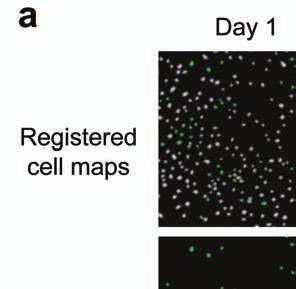
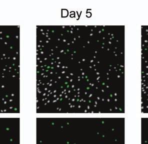
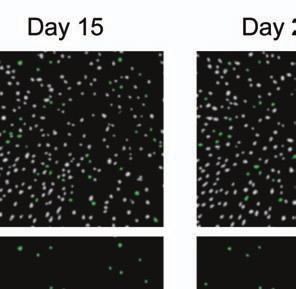
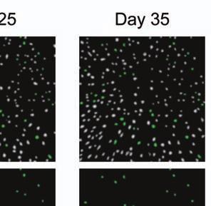
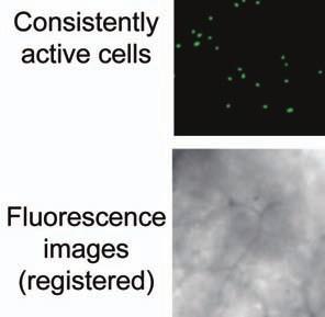
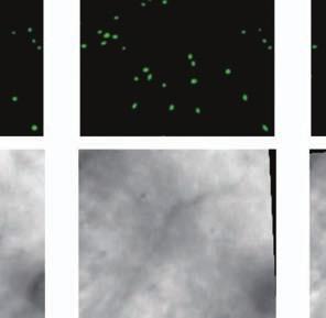
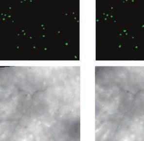
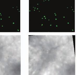
4 Supplementary Fig. 3 Image registration had 1-µm accuracy and enabled identification of the same CA1 neurons for over a month. (a) Image registration permitted repeated detection of the same individual cells despite substantial turnover in the population of detected cells between sessions. For each imaging

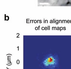
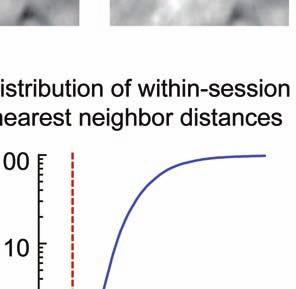
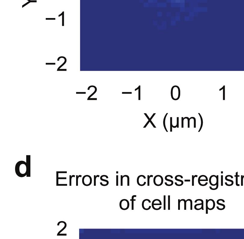
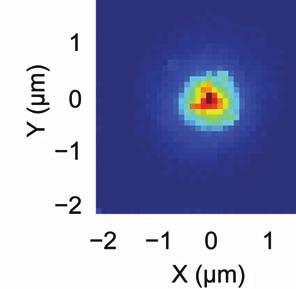
5 session, we created an initial map containing all cells found in that session (Online Methods). We used standard image alignment methods to cross-register these maps to each other (top row), using the map from a single day (usually day 15) as a reference. A subset of cells was repeatedly detected in every session (green cells in top row and middle row). The realigned fluorescence images (bottom row), attained by using the same coordinate transformations as for the cell map cross-registrations, gave visual confirmation of the alignments. Scale bar is 100 µm. (b, c) Errors in alignment of the individual cell maps to the reference map were nearly always <1 µm. We estimated the variance in alignment results by using a bootstrap analysis of nine cell maps and one reference map obtained from an individual mouse over ten imaging sessions. For each of the nine cell maps we performed the alignment procedure 1000 times using a distinct, randomly chosen 50% of the cells each time. The histogram, (b), and cumulative distribution, (c), of the differences in the alignment results revealed that the standard deviation of the alignment was sub-micrometer in magnitude. (d, e) Errors in the cross-registration of the cell maps from different imaging sessions were nearly always <1 µm. We estimated the variance in cross-registration by changing the session that provided the reference map. After re-doing the cross-registration ten times, with each of the ten days serving once as the reference, we tabulated the differences in the centroid coordinates for all n = 10,039 cells observed across 4 mice and 10 imaging sessions. This yielded n = 90,351 pairs of x-y coordinate displacements. The histogram, (d), and cumulative distribution, (e), of these displacements revealed that the standard deviation of the cross-registration was submicrometer in magnitude. (f) Cumulative distribution of nearest-neighbor distances within individual imaging sessions revealed that centroids of CA1 pyramidal cell bodies were always separated by 6 µm (red

6 dotted line). Thus, given that the errors in our alignment and cross-registration procedures were nearly always at the sub-micrometer scale, we assigned the same identity to those cells from two or more distinct imaging sessions with <6 µm between their centroids.

7 Supplementary Fig. 4 Activity-related parameters predict neither the re-appearance of neurons across imaging sessions nor the odds that CA1 neurons retain place fields. (a, b) Neither the mean frequency, (a), nor the mean amplitude, (b), of Ca 2+ activation predicted the number of imaging sessions in which CA1 neurons would actively appear (Pearson's r values of 0.00, and 0.28, respectively). Each data point represents an individual cell, which is marked with the same color in panels c and d. We extracted mean rates and amplitudes of Ca 2+ activation from periods when the mouse actively walked or ran along the track. (c, d) Among those sessions in which a cell was detected, neither the mean frequency, (c), nor the mean amplitude, (d), of Ca 2+ activation predicted the fraction of sessions in which the cell s Ca 2+ activation activity encoded a statistically significant place field (r values of 0.17, and 0.18, respectively). Each data point represents an individual cell, with the color indicating the number of sessions in which the cell had detectable activity.

8 Supplementary Fig. 5 The coding properties of cells with especially stable place fields in individual imaging sessions evolve similarly over the long-term as other place cells. To check whether our basic results about place cell turnover might depend on the degree to which cells coding properties were stable within individual sessions, we identified subsets of cells whose place fields met especially strict stability criteria. We used the same computational procedures that we had used to identify statistically significant place fields (Online Methods), except that we applied these procedures separately to the first and second halves of the mouse s time spent moving within a session. We required the place field to be statistically significant within each half of the data (20,000 temporal shuffles for each half) and that the place fields centroids in each half of the data were within 7 cm of each other. Restriction of the main analyses to the subset of cells that passed these stricter criteria did not alter our core findings. (a) If a cell displayed Ca 2+ activity in one imaging session, the odds that this cell also had Ca 2+ activity in a subsequent session declined with the temporal interval between the two. The data points marked by solid blue circles are identical to those of Fig. 3c and express mean ± s.e.m. values determined from all cells in the experiment. The open circles denote mean values computed over a subset (~30%) of the cells that had especially stable place field attributes within the first of the two days being considered. The close similarity of the two curves indicates that

9 cells with especially stable place coding attributes within an imaging session show nearly the same odds of having detectable Ca 2+ activity in subsequent sessions as do the cells without these initial attributes. (b) If a cell had a statistically significant place field in one imaging session, the odds that this cell had a statistically significant place field in a subsequent session also declined with time. Solid red data points are for all cells in the experiment and are identical to those in Fig. 3c. Open red data points are for the ~30% subset of cells that met the same within-session stability criterion used in panel a. (c) If they reappeared, the subset of cells with especially stable place coding within individual sessions did not shift their centroid locations between imaging sessions, regardless of the temporal interval between the two sessions. The distributions of shifts (colored according to the interval between sessions) for this subset of cells were thus statistically indistinguishable (Kolmogorov-Smirnov test; P = ) from those for all cells with statistically significant place fields (Fig. 3d). Black data points are the expected shifts based on the null hypothesis that place fields locations would randomly relocate. Inset: Cumulative histograms of the magnitudes of centroid displacements.

10 Supplementary Fig. 6 The long-term evolution of place-coding properties is robust to changes in the threshold used for cell identification. The long-term dynamics of whether cells retained place coding attributes were impervious to increases in the stringency for extracting cells from the Ca 2+ imaging video data. As a control, we ran the cell sorting procedure ten separate times, with a different random seed each time for the independent components analysis (ICA). 90% of all cells were identified at least nine of ten times, indicating that very few if any cells are of marginal quality. When we restricted subsequent analyses to the 70% of cells that were present in all ten rounds of cell identification, the probabilities of a cell reappearing within the active and place-coding ensembles were unchanged. Blue and red data points (mean ± s.e.m.) are the same as those in Fig. 3c for the full data set and are nearly indistinguishable from the data (black points) for the cells found in all ten iterations of ICA.

11 Supplementary Fig. 7 Inclusion of the amplitudes of Ca 2+ -activation in the data analyses did not alter conclusions regarding the time-evolution of neural coding. (a g). We calculated additional versions of the plots of Figs. 2f h and 3d g in which we weighted each Ca 2+ transient in proportion to its amplitude. The graphs were hardly changed from the un-weighted versions and the conclusions were unaltered.

12 Supplementary Fig. 8 Bayesian decoding of place cells Ca 2+ dynamics permits accurate reconstruction of the mouse s trajectory. We used conventional Bayesian methods 27,28 to estimate the mouse s most likely present location given the most recent 800 ms (16 time bins) of neuronal Ca 2+ activity. Our formulation had the simplifying assumption that the probabilities of finding a Ca 2+ transient for any of the N cells

13 within any of the 16 time bins were independent of one another. (In principle, a decoder that did not assume this form of independence could provide superior reconstructions of the mouse s position, but the amount of Ca 2+ -imaging data required to properly train the decoder rises approximately exponentially with the number of statistically interdependent cells). We thus estimated the position, ŷ, of the mouse at time t using ŷ(t) = arg max y N 15 i=1 j=0 ( ) p y p( x ij (t)) p x ij (t) y ( ), where y denotes the position on the linear track, binned in 3.5-cm increments but excluding the last 7 cm at each end. Here x ij (t) is a binarized indicator of the activity of cell i at time t-j, where 1 indicates the presence of a Ca 2+ transient and 0 indicates the lack thereof. p(y) and p(x ij ) denote unconditional probabilities, as estimated from the data used to train the decoder. p(x ij y) is the conditional probability that cell i had activity level x ij whenever the mouse was at position y. To convert the continuous traces of Ca 2+ activity into binary form, we set x ij to 1 if cell i had a Ca 2+ transient in the time interval [t-j-f b r, t+j+f a r], where r is the rise time of the transient and f a and f b are fractions (range: ). We separately optimized and fixed f a and f b for each mouse, although the sensitivity of decoding performance to these two parameters was low. To train a decoder, we used two trials of data (3 min each) taken from the same mouse and imaging session. From these two trials we empirically determined the probabilities p(y), p(x ij y), and p(x ij ) by counting the respective occurrence frequencies. To test the ability of the resulting decoder to estimate the mouse s location, we used a separate data trial from either the same or a different experimental session. In the latter case we used only the cells that had statistically significant place fields on both days.

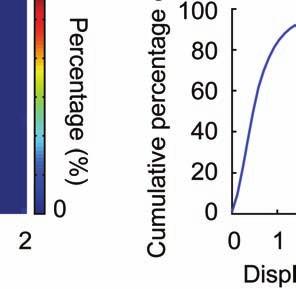
14 (a) Bayesian decoding of neural traces of [Ca 2+ ]-sensitive fluorescence enabled reconstructions of the mouse s trajectory. We first converted the neurons dynamical traces to a binary format with a time step, Δt, of 50 ms. 0 s indicated quiescence and 1 s marked the rising portion of a Ca 2+ -transient. To determine the mouse s position at time t, the decoder used the entries of the neurons binary traces at t, as well as those at t-δt, t-2δt, t-3δt, t-15δt. (The diagram schematizes this only up to two previous time bins). Using a filter previously optimized on separate data, the decoder estimated the mouse s location as the most likely position on the track (binned in 3.5-cm increments) given the cells binarized [Ca 2+ ] data. (b) Example reconstructions of the mouse s position as a function of time (red curves) plotted atop the mouse s actual position (black curves). The four examples are from three different mice, studied on four different days. We trained each decoder on separate trials from those used for testing its reconstruction capabilities but acquired on the same day. (c, d) We assessed each decoder s performance on a trial-by-trial basis via determination of the median error over all time points in the reconstruction of the mouse s position. The error was defined as the absolute value of the difference between the actual and estimated location of the mouse. To assess the statistical significance of decoders performance, we applied the same decoding procedures on temporally shuffled data sets in which Ca 2+ transients were randomly assigned within the data segments used for reconstruction. Median errors in reconstruction of the mouse s position are usually <7 cm, i.e. <9% of the track s total length. (c) Cumulative distributions of the magnitude of reconstruction errors in the estimation of the mouse s position. The blue curves show the cumulative distributions for individual behavioral trials on the running track. The red curve shows the mean over all trials (mean ± s.e.m.; n = 63 trials for n=3 mice). The gray line shows the cumulative distribution of reconstruction errors for shuffled versions of

15 the data, in which the times of all Ca 2+ bursts for each cell were uniformly randomized (mean ± s.e.m.; n = 63 trials with 10,000 shuffles each). (d) Histogram of the median reconstruction error (blue bars) reveals decoding is much more accurate for the real Ca 2+ -imaging data than the shuffled data (gray bars) and shows only a small minority of trials have a median error >7 cm. To benchmark the time-lapse decoders (Fig. 3h-j), we paired each time-lapse decoder with a same-day decoder trained on data from the identical day as the test data. We chose cells for this same-day decoder by rank ordering cells according to the mutual information between their Ca 2+ excitation events and the mouse s location. We took cells from the top of this list until the total selected equaled the number of cells in the time-lapse decoder. This permitted fair comparisons between each time-lapse decoder and an optimally constructed, same-day decoder with the same number of cells. We verified that selecting cells by their mutual information scores provided a reasonable approximation of optimality, for we achieved similar decoding performance by examining 10,000 random subsets of cells and taking the subset with the lowest decoding error.