Analysis of Genome-wide association studies (GWAS)

Transcription

1 Basic skills for genetics research - 19 th January, 2017 Analysis of Genome-wide association studies (GWAS) Clara Tang Department of Surgery Faculty of Medicine Dr Li Dak-Sum Research Centre

2 Genetic variation and disease The differences in DNA sequence between 2 individuals may be highly relevant to phenotypic differences differences in anatomy, physiology, psychology and diseasepredisposition What creates genetic variation? Mutation : introduces novel variant into the population Recombination/crossing over : re-shuffles the existing patterns of variation The fate of new mutations is affected by genetic drift, nature selection and population history

3 Common variation Rare variation Abundance ~ ? Selection Unlikely Possible Population specific? No Often Best technology SNP array genotyping Sequencing

4 time Consequences of mutation & recombination Genetic variants are correlated because they share a history of inheritance Without recombination, this correlation would extend a great distance along chromosomes Mutation causal to disease A Recombination breaks down this correlation over successive generations, leaving a narrower window of correlation Linkage disequilibrium (LD) Polymorphism (e.g. SNP)

5 LD and indirect association LD is defined as the association between alleles at closely linked loci Causal variant This SNP is highly correlated or in linkage disequilibrium with the causal variant Due to incorrect association, this SNP is also associated with disease A

6 Haploview Plot Red: high LD between SNPs Recombination hotspots Nature 526, (2015) LD decays by genetic distance as chance of recombination increases Nature 437, (2005)

7 Quantifying LD

8 Quantifying LD Tagged markers that can be pairwise tagged in a specified population at r 2 0.8

9 Applying HapMap LD pattern in GWAS design Barrett and Cardon, Nat Genet, 2006 Nature (2005)

10 Common variation Rare variation Abundance ~ ? Selection Unlikely Possible Population specific? No Often Correlation High Low Best technology SNP array genotyping Sequencing

11 SNP array Genotyping by SNP array Genome-Wide Association Study and copy number analysis Genetic study of mostly common DNA variations OmniZhongHua/ Multi-ethnic Illumina exome/coreexome chip Affymetrix Axiom Exome

12 Low frequency variants with intermediate effect Common variants with small effect GWAS Adapted from Manolio et. al. (2009) and Zemunik et. al. (2011)

13 Genome-wide association analysis (GWAS) Association analysis compares frequency of alleles or genotypes of a variant between cases and controls/across quantitative traits GWAS is an unbiased approach to detect association of variants in LD with the causal variants Mathew. Nat Rev Genet 9, 9-14 (2008); Hirschhorn & Daly. Nat Rev Genet 6, (2005)

14 Factors affecting success of GWAS Genetic architecture Genotyping platform Ascertainment of samples Power Power Nβp(1-p)r 2 N = sample size β = effect size (beta estimate/odds ratio) p = frequency r 2 = correlation (LD) to causal variant

15 GPC Genetic Power Calculator: design of linkage and association genetic mapping studies of complex traits Purcell, Cherny and Sham (Bioinformatics, 2003) ~purcell/gpc/

16

17

18 GWAS : statistical analysis Family-based GWAS Transmission disequilibrium test (TDT) Mixed-model association analysis Case-control analysis Controls Cases Population-based GWAS Testing of association in unrelated individuals Binary trait: Case-control association analysis Allele-based test Genotypic test Logistic regression (with/without covariates) Quantitative trait: Quantitative trait locus (QTL) association analysis Linear regression T/T T/T T/TT/G T/T T/T T/G QTL analysis Positive association No association G/T G/G T/G T/G T/G G/G T/G Allele G is associated with disease Negative association

19 A GWAS dataset Summary statistics and quality control Assessment of population stratification Whole genome SNP-based association Whole genome haplotype-based association Visualization Further exploration of hits Follow-up

20 Recombination rate (cm/mb) GWAS : PLINK / PLINK2 Locuszoom Regional plot r log 10(p value) HMGCR rs P TC = FAM169A ANKRD31 HMGCR POLK POC5 GCNT4 COL4A3BP ANKDD1B Position on chr5 (Mb) QQ (quantilequantile) plot Manhattan plot Purcell, Sham et al. AJHG 81(3): (2007); Tang et al. Nat Commun (2015)

21 PLINK genotype files plink --file text_fileset --out binary_fileset Text fileset (--file :.ped +.map files Binary filesset (--bfile :.bed +.bim +.fam files).fam.ped.map.bim 1) FID : family ID 2) IID : Individual ID 3) Paternal ID 4) Maternal ID 5) Sex (1 Male; 2: Female) 6) Phenotype Only for.ped 7- SNP genotypes 1) Chromosome 2) SNP id 3) Genetic distance (morgans) 4) Base-pair position (bp) For.bim 5) A1: minor allele 6) A2: major allele

22 People SNPs Genotypes Data management SNPs P1 A A A C C G T T A A T T P2 A C A A C G G T A C T T P3 C C A C G G T T A A T T P4 C C A A G G G T A A T T People S1 A A A C C C C C S2 A C A A A C A A S3 C G C G G G G G S4 T T C G T T G T S5 A A G T A A A A S6 T T A C T T T T P1 S1 A A P1 S2 A C P1 S3 C G P2 S4 A C P2 S5 C C S1 S2 S3 S4 P P2 0 NA 0 2 P P Numeric coding S1 A/A P1 P2 P7 P8 S1 A/C P3 P4 S1 C/C P5 S2 G/T P5 S2 G/G P1 P2 P3 P4 List by genotype Compact binary format Recode dataset (A,C,G,T 1,2) Reorder, reformat dataset Flip DNA strand Extract/remove individuals/snps Swap in new phenotypes, covariates Filter on covariates Merge 2 or more filesets P1 S1 A 2 C 0 P1 S2 A 1 C 1 P1 S3 C 0 G 1 P2 S4 A 3 C 1 P2 S5 C 2 C 2 SNPs in CNPs

23 Summary statistics Filters and reports for standard metrics Missing rate (by variant/individual) Hardy-Weinberg Mendel errors Allele frequency Tests of non-random missingness by phenotype and by (unobserved) genotype Individual homozygosity estimates Check/impute sex based on X chromosome

24 One of the most famous GWAS GWAS study of exceptional longevity (EL) 1) Large effect size for the significant SNPs 2) Abnormal Manhattan Plot Science centenarians and 1267 controls A genetic model that includes 150 single nucleotide polymorphisms (SNPs) was built, which could predict EL with 77% accuracy in an independent set of centenarians and controls.

25 Science Nature 447,

26 Adapted from Dr Jeff Barrett, at IBG 2015, Boulder

27 PLoS One. 2012

28 Quality control : we need clean data! Variant-based QC Call rate / missingness Hardy Weinberg equilibrium

29 Genotyping rate plink --file mygene --missing Per-individual genotyping/missing rate, plink.imiss FID IID MISS_PHENO N_MISS N_GENO F_MISS per0 per0 N per1 per1 N per2 per2 N per3 per3 N per4 per4 N per5 per5 N per6 per6 N per7 per7 N Per-marker (locus) genotyping/ missing rate, plink.lmiss CHR SNP N_MISS N_GENO F_MISS 1 rs rs rs rs rs rs rs rs plink --file mygene --mind geno 0.05

30 Quality control : we need clean data! Hardy Weinberg equilibrium For large population under random mating Allele frequencies for allele A and a in the offspring, denoted as p and q, are the same as those in the parental generation Genotype frequencies in the offspring will follow the ratios p 2 :2pq:q 2 for Aa:Aa:aa Alleles A a A p2 pq p a pq q2 q p q

31 Hardy-Weinberg disequilibrium plink --file mygene --hardy Output file plink.frq CHR SNP TEST A1 A2 GENO O(HET) E(HET) P 1 rs00001 ALL G C 44/463/ rs00001 AFF G C 17/219/ rs00001 UNAFF G C 27/244/ rs00002 ALL C A 34/509/ rs00002 AFF C A 17/257/ rs00002 UNAFF C A 17/252/ rs00003 ALL A T 415/772/ rs00003 AFF A T 215/474/ rs00003 UNAFF A T 200/298/ rs00004 ALL G C 363/952/ rs00004 AFF G C 178/485/ rs00004 UNAFF G C 185/467/ rs00013 ALL G A 567/512/ e-96 1 rs00013 AFF G A 277/0/ e rs00013 UNAFF G A 290/512/ plink --file mygene --hwe 1e-4

32 Quality control : we need clean data! LD pruning --indep-pairwise Individual-based QC (after --extract plink.pruned.in ) Call rate / missingness --missing Biological relationship Heterozygosity Sex check --mendel / --genome Relationship IBD2 IBD1 IBD0 PI-hat MZ/Duplicate Parent-Offspring Full sibling/dz 1/4 1/2 1/4 0.5 Half sibling/uncle-nephew 0 1/2 1/ First cousin 0 1/4 3/ Unrelated het --check-sex

33 Quality control : we need clean data! Sample-based QC 4 Low quality DNA samples 4 Unexpected relatives / incorrect biological relationship 4 Duplicates 4 Sample mix-ups 4 Gender mismatch 4 Samples with different ancestry

34 Quality control : we need clean data! Sample with different ancestry SNP 1 Chinese European Freq A =60% Freq a =40% A a Freq A =20% Freq a =80% A a McCarthy et al. (2008) Nature Genetics Alleles Chinese European Count of A Count of a Case = = 120 Controls = = 160 False positive due to population stratification Odds ratio=2.69; Chi-square P=2.1x10-5

35 Quantile-quantile (QQ) plot McCarthy et al. (2008) Nat Genet Genomic control (λ)=1.00 λ=1.15 λ=1.15 λ=1.02 Little evidence of association Population stratification Cryptic relatedness Very polygenic vs polygenic Excess of strong associations Genomic control (λ) mean (chi-square statistics) median (chi-square statistics) / Genomic control (λ) close to 1 implies no/little population stratification

36 Quantile-quantile (QQ) plot McCarthy et al. (2008) Nat Genet Genomic control (λ)=1.00 λ=1.15 λ=1.15 λ=1.02 Little evidence of association Population stratification Cryptic relatedness Very polygenic vs polygenic Excess of strong associations Plots observed log(p) or chisq statistics, ranked in magnitude, against their expected values according to the null hypothesis If the null hypothesis is true for all SNPs (Fig a) and the tests are behaving appropriately, then the plot should follow the line of equality Deviations from the null line may suggest Misbehaviour of statistical tests, e.g. population stratification (Fig b) The presence of true associations (Fig c and d)

37 Principal Components Analysis (PCA) Principal Components Analysis (PCA) is applied to genotype data to infer continuous axes of genetic variation E.g. EIGENSTRAT Each axis explains as much of the genetic variance in the data as possible and each component is orthogonal to the preceding components The top principal components (PCs) tend to infer population structure We can include PCs as covariates in regression analysis to correct for the effects of population stratification

38 Second Principal Component Novembre et al, Nature (2008) First Principal Component

39 Am J Hum Genet Dec 11; 85(6):

40 Association analysis (allelic) plink --file mygene --assoc Output file plink.assoc CHR SNP BP A1 F_A F_U A2 CHISQ P OR 1 rs G C rs C A rs G C rs C T rs T A rs G A rs T G rs T C rs A C rs C G 8.647e rs C T rs A G rs A C

41 Corrections for multiple testing plink --file mygene --assoc --adjust Output file plink.assoc.adjust: rs00008 is significant after Bonferroni correction CHR SNP UNADJ GC BONF HOLM SIDAK_SS SIDAK_SD FDR_BH FDR_BY 1 rs rs rs rs rs rs rs rs rs rs rs rs rs

42 Tests of association at rs00008 plink --file mygene --snp rs model Calculates allelic, trend, genotypic, dominant and recessive tests: plink.model Reports results in plink.assoc.logistic CHR SNP A1 A2 TEST AFF UNAFF CHISQ DF P 1 rs00008 T G GENO 19/235/728 14/172/ rs00008 T G TREND 273/ / rs00008 T G ALLELIC 273/ / rs00008 T G DOM 254/ / rs00008 T G REC 19/963 14/ plink --file mygene --snp rs logistic --interaction --sex Reports results in plink.assoc.logistic Or test SNP-by-sex interaction, using logistic model CHR SNP BP A1 TEST NMISS OR STAT P 1 rs T ADD rs T SEX rs T ADDxSEX

43 Both rs00008 and rs00009 are associated P<0.01 and are also in moderately high LD with each other. Are these two associations independent? plink --file mygene --logistic --condition rs00008 Includes genotype at rs00008 as a covariate; results in plink.assoc.logistic CHR SNP BP A1 TEST NMISS OR STAT P 1 rs G ADD rs G rs rs C ADD rs C rs Often desirable to extract out only the terms for the SNP (ADD) grep -w ADD plink.assoc.logistic 1 rs G ADD rs C ADD rs G ADD rs C ADD rs T ADD rs G ADD rs T ADD 1968 NA NA NA 1 rs T ADD rs A ADD rs C ADD rs C ADD rs A ADD rs A ADD

44 Determine pattern of linkage disequilibrium in the region plink --file mygene --r2 Calculates pairwise LD (r 2 ) between all SNPs; by default, only output only pairs with r 2 > 0.2, to file plink.ld CHR_A BP_A SNP_A CHR_B BP_B SNP_B R rs rs rs rs plink --file mygene --ld rs00008 rs00009 LD information for SNP pair [ rs rs ] R-sq = D' = Haplotype Frequency Expectation under LE GC AC GT AT In phase alleles are GT/AC

45 Recombination rate (cm/mb) Visualization of association analysis result Manhattan plot GWAS significance threshold P<5x10-8 based on multiple testing QQ (quantilequantile) plot - log 10 (p value) r Regional plot HMGCR rs P TC = FAM169A ANKRD31 HMGCR POLK POC5 GCNT4 COL4A3BP ANKDD1B Position on chr5 (Mb)

46 Manhattan plots GWAS significant Nature 511, (24 July 2014) GWAS significance threshold P<5x10-8 based on estimated number of ~1million independent tests across the genome

47 - log10(p value) Combined P=2.6x10-77 RET rs P = MIR5100 RET RASGEF1A CSGALNACT2 Tang et al. HMG (in press) - log10(p value) ZNF33B LOC BMS1 MIR5100 RET RASGEF1A FXYD4 CSGALNACT2 ZNF239 HNRNPF Position on chr10 (Mb) r European RET rs P = ZNF33B LOC BMS1 MIR5100 RET RASGEF1A FXYD4 CSGALNACT2 ZNF Position on chr10 (Mb) ZNF239 HNRNPF ZNF Position on chr10 (Mb) 44 Recombination rate (cm/mb) 40 Asian RET rs P = Recombination rate (cm/mb) 50 r2 - log10(p value) Recombination rate (cm/mb) Regional plots (Locuszoom plots) r2

48 Replication Replicating the genotype-phenotype association on independent sample is the gold standard for proving an association is genuine The replicated signal should be in the same direction Preferably using independent platform and samples of similar or independent population Most loci underlying complex diseases will be of small to moderate effect Two-stage design 1 st discovery stage : more SNPs but less samples 2 nd replication stage : top SNPs (n<100) but more samples Joint analysis can be more powerful, i.e. a lower p-value, than the original report

49 Progress of genetic studies of complex diseases Number of loci reaching genomewide significance seems to increase at least linearly with increasing sample size Multiple GWAS using different genotyping platforms, of different ethnic groups can be metaanalyzed to increase power for detection of association DIAGRAM, CARDIoGRAM, MAGIC, GIANT Visscher et al., AJHG (2012)

50 Meta-analysis of GWAS Combine data from multiple studies to increase statistical power obtain more precise effect size estimates Combine summary statistics, rather than raw genotype, from each study Fixed-effect Inverse variance approach Assumption : one underlying true effect that all observed differences in effects are by chance Random-effect approach Assumption: true effect size might differ from study to study software : METAL, METASOFT, GWAMA

51 Inverse variance weighted method Computing pooled effect: Pooled effect= Sum (weights * effect estimates) Sum (weights) b pooled = N å i = 1 ( w * b N å i = 1 i ( w i ) i ) w i = var( 1 b i ) var( b ) = se ( b i i se ( b ) = i SD n i i ) 2 i=1 N samples M. de Moor, Boulder March 2009

52 Inverse variance weighted method Computing pooled standard error: 1 Pooled standard error = Square root( ) Sum (weights) se pooled = N å i = 1 1 ( w i ) w i var( = var( 1 b b ) = se ( b i i i ) ) 2 M. de Moor, Boulder March 2009

53 Inverse variance weighted method Computing test statistic: c 2 df b pooled = = = 1 2 se pooled 2 N å ( w * b i = 1 N å i i = 1 w i i ) 2 z = b se pooled pooled = N å i = 1 w N å i i = 1 * b w i i M. de Moor, Boulder March 2009

54 Do assumptions of fixed-effect model hold? Test of homogeneity Cochran s Q statistic Q = N å i = 1 w i ( b - b i pooled ) 2 χ 2 -distributed with df=k-1 k=number of samples I 2 statistic measures the percentage of the variability in effect estimates that is due to heterogeneity I 2 = Q - ( k Q - 1) * 100 Range 0-100% I 2 > 50%: Large heterogeneity I 2 > 75%: Very large heterogeneity M. de Moor, Boulder March 2009

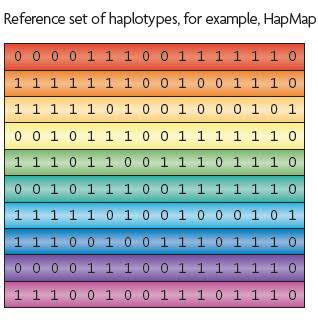
55 Imputation Reference panel e.g. HapMap, 1000 Genomes Marchini & Howie (2010)

56 The 1000 Genomes Project The goal of the project was to find most genetic variants with frequencies >=1% in the populations studied It is now a catalog of ~2500 genomes With its introduction, HapMap becomes less frequently used and eventually retired on 16 June, 2016

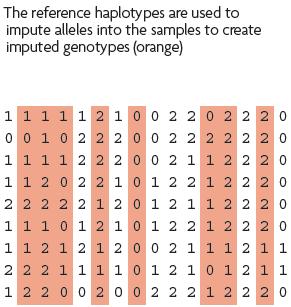
57 Imputation Why do we need imputation? o Most commonly used for Combining data from different chips Meta-analysis Fine Mapping o Less commonly used for imputation of missing genotypes correction of genotyping errors imputation of non-snp variation (e.g. indels)

58 Imputation

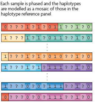
59 Imputation (Pre-)Phasing - haplotype estimation Use genotype data to reconstruct the best-guess haplotypes Can use reference data and its haplotype frequency to improve accuracy Imputation Compute the genotype probabilities for missing SNPs Software Mach + minimac SHAPEIT2 + IMPUTE2 Beagle

60 The Haplotype Reference Consortium

61 The Haplotype Reference Consortium Free imputation and phasing servers to use the full haplotype reference panel to impute missing genotypes in their data Imputation servers Users can upload genotype data to the server Imputed data can be downloaded after the imputation Phasing server for phasing high coverage sequenced samples A subset of the full haplotype panel is now available through EGA

62 Post-GWAS analysis Set-based (Gene-based/Pathway-based) tests Prioritization of causal genes DEPICT : prioritizes the most likely causal genes at associated loci, highlights enriched pathways, and identifies tissues/cell types where genes from associated loci are highly expressed PrediXcan : estimates the component of gene expression determined by an individual's genetic profile and correlates 'imputed' gene expression with disease traits Heritability/Phenotypic variance explained by GWAS GCTA, LD score regression Mendelian randomization

63 Challenges to GWAS Unmatched controls / population structure Data quality control Sample/effect size too small to detect effects Meta-analysis to leverage power SNP chips don t cover enough of the genome Genotype imputation to recover missing variants No common, single SNP main effects o Effect of rare variants or through interaction o Next generation sequencing (NGS)