Genome Wide Association Study for Binomially Distributed Traits: A Case Study for Stalk Lodging in Maize

Transcription

1 Genome Wide Association Study for Binomially Distributed Traits: A Case Study for Stalk Lodging in Maize Esperanza Shenstone and Alexander E. Lipka Department of Crop Sciences University of Illinois at Urbana-Champaign

2 Unified Mixed Linear Model (MLM) in GWAS Grand Mean Marker effect Random effects: account for familial relatedness Phenotype of i th individual Fixed effects: account for population structure Observed SNP alleles of i th individual Random error term Measures relatedness between individuals Adapted from A. Lipka Yu et al. (2006) 2

3 Assumptions of the Unified MLM What do we do if these assumptions cannot be met? (Example: Binomially distributed data) Adapted from A. Lipka Yu et al. (2006) 3

4 Binomial Distribution: # Successes in n Independent Success/Failure Trials Mixed Logistic Regression does not require normality or equal variances Problem: Fitting this model is extremely Conduct GWAS by fitting a logistic regression model at each SNP computationally intensive!!! Logit Link function: The natural log-odds of a mean success The grand

5 Purpose Develop a multi-model GWAS approach that will allow mixed model GWAS to be conducted on binomially distributed traits 5

6 Stalk Lodging In Maize Stalk Strength Disease/Pests Environmental Factors 5-20% yield losses worldwide Flint-Garcia et al.,

7 Data Collection Two Reps of the Goodman-Buckler diversity panel were planted using incomplete block design The entire experiment was inoculated with Goss s wilt In this experiment there was no correlation between disease and lodging The Jamann Lab at UIUC 7

8 Lodging Phenotyping Standcount Number of Plants Lodged Number of plants Not lodged Lodging Score (Percent Lodged) % End Beginning of growing of season Growing Season Above: Diagram depicting one plot (rep) of one taxa in the field 8

9 Treat Lodging Data as a Binomial Setup of Binomial The experiment consists of n repeated trials Each trial has two outcomes: success or failure The probability of success, π, is the same on every trial The trials are independent Why we think binomial is an appropriate approximation for lodging Within each plot, each plant is a trial Success: plant has lodged Failure: Plant has not lodged The probability of a plant lodging, π, is the same within a plot One plant lodging will not change the likelihood of another plant lodging 9

10 Multi-Model Approach Model 1 Fit Logistic Regression Model Controls for population structure only Identify peak SNPs Model 3 Fit Mixed Logistic Regression Model Using Peak SNPs from Model 1 and Model 2 Model 2 Fit a Mixed Linear Model Controls for population structure and relatedness Identify peak SNPs 10

11 Logistic Regression Identified ~50% of Markers to be Significant Peak SNP Possible SNPs of interest The top 2,796 SNPs from this model were subset RStudio Chromosome Motivation: mixed logistic regression model can fit 2,796 models in < 1 day 11

12 Unified MLM Identified No Significant Signals GAPIT Lipka et al., 2012 Chromosome 12

13 Mixed Logistic Regression Identifies 68% of SNPs Identified in Logistic Regression to Be Significant Accounting for familial relatedness helped refine location of putative genomic regions SAS 9.4 PROC GLIMMIX Chromosome Signals coincide with those previously identified for traits related to lodging 13

14 Simulation Study in Goodman- Buckler Diversity panel: Determine which parameters of the binomial distribution contribute the most to identification of genomic signals 14

15 Proposed Methodology for Simulation Study Assign SNP from 4K Set to be QTN Simulate binomial distributed trait QTN Effect size Stand count per plot Grand mean For each trait in each setting: Simulate Data~100 Traits Assessed genomic positions of top 100 markers with strongest associations Fit logistic regression model at each of 55K SNPs 15

16 How does the total number of plants in a plot affect QTN detection? Stand Count: 10 Top 100 SNPs from each trait used to create this figure Proportion of times detected: 1.0 Model 1

17 How does the total number of plants in a plot affect QTN detection? Stand Count: 15 Top 100 SNPs from each trait used to create this figure Proportion of times detected: 1.0 Model 1

18 How does the total number of plants in a plot affect QTN detection? Stand Count: 20 Top 100 SNPs from each trait used to create this figure Proportion of times detected: 1.0 Model 1

19 How does the total number of plants in a plot affect QTN detection? Stand Count: 25 Top 100 SNPs from each trait used to create this figure Proportion of times detected: 1.0 Model 1 Stand count does not appear to affect our ability to detect QTN

20 Top 100 SNPs from each trait used to create this figure How does grand mean affect QTN detection? Grand Mean = 0 ; P{Success} = 0.5 Proportion of times detected: 1.0 Model 1

21 Top 100 SNPs from each trait used to create this figure How does grand mean affect QTN detection? Grand Mean = 1; P{Success} = 0.73 Proportion of times detected: 1.0 Model 1

22 How does grand mean affect QTN detection? Grand Mean = 3; P{Success} = 0.95 Top 100 SNPs from each trait used to create this figure Proportion of times detected: 0.82 Model 1

23 How does grand mean affect QTN detection? Grand Mean = 5; P{Success} = 0.99 Top 100 SNPs from each trait used to create this figure Proportion of times detected: 0.10 Model 1 Grand mean values affects our ability to detect QTN

24 Future Directions Any phenotype that measures # successes in a plot of n plants could theoretically use these approaches - Try to design experiments that result in a baseline probability of success of 0.5 How can we fit mixed linear models in a computationally efficient manner on a Windows/Mac computer? - Temporary solution: multi-model approach is reasonable - Try to strive for: write software that uses the score test 24

25 Acknowledgements Committee Members Dr. Alexander E. Lipka Dr. Tiffany Jamann Dr. Martin Bohn Dr. Pat Brown The Jamann Lab Julian Cooper Graduate Students Amanda Owings Department of Crop Sciences at UIUC The Lipka Lab Brian Rice Angela Chen 25

26 Model 1 vs. Model 2 Comparison

27 Varying Additive Effect Sizes (Same Assigned QTN) Additive effect size 0.5 on chromosome 8 Proportion time detected: 0.93 Additive effect size 0.1 on chromosome 8 Proportion of times detected:0.07

28 Summary of Results Able to identify two significant SNPs in the BP region of Maize Stalk Strength QTL Li et al., 2014, Flint-Garcia et al., 2003, Hu et al., 2012 Peak SNPs on Chromosome 7 were in the same location as the most robust marker association with RPR Pieffer et al., 2013 A significant SNP on Chromosome 1 was in the same region as a candidate gene for Mediterranean Corn Borer stalk destruction susceptibility Samayoa et al.,

29 High LD Decay Observed AroundPeak SNP on Chromosome Seven 29

30 Limiting Factors of This Study Stalk lodging is a putatively low heritability trait No repeatability across replications Only one year of data included in this analysis Only one environment Missing data Various factors contributed 30

31 Summary of Project Logistic Regression is computationally intensive Approximately 30 seconds to run 1 SNP in SAS ~17.36 days to run 50,000 SNPs Model 1 and Model 2 are used to identify which SNPs are fit using the complete logistic regression model (Model 3) The number of SNPs to include is dependent on computational power available Stalk Lodging data was used to test this approach Some Peak SNPs identified are in the same region as QTL associated with stalk strength, and a candidate gene for MCB Stalk Damage 31

32 Data Collection Reps of the 282 diversity panel were planted using incomplete block design The entire experiment was inoculated with Goss s wilt In this experiment there was no correlation between disease and lodging The Jamann Lab 32

33 Observed Lodging in the Field Taxa classified as non stiff stalk were lodged more often Taxa classified as stiff stalk were lodged the less often All plots represented in this graph had at least 10 plants lodged 33

34 Lodging Score Residuals Follow a Non-Normal Distribution The Box-Cox procedure was implemented, and λ=-0.6 was the suggested transformation Transformation was unsuccessful Frequency Distribution of Lodging Scores 352 plots had no lodging Lodging Score 34

35 Genome-Wide Association Study (GWAS) Search the genome for genetic markers significantly associated with your trait of interest Allows for the identification of QTLs region of the genome associated with the trait / Single Nucleotide Polymorphism (SNP): A type of genetic marker 35

36 282 Diversity Panel ~75% of all allelic diversity in Maize Romay et al., 2013 Adapted from Flint-Garcia et al.,

37 Outline Introduction Genome-Wide Association on Stalk Lodging in Maize Simulation Study Conclusions 37

38 Unified Mixed Linear Model Controls for False Positives Flowering time of Maize (High population structure) Simple Ear Diameter of Maize (Low Population Structure) Simple Yu et al.,

39 Stalk Lodging in Maize Predicting lodging is challenging Most methods are destructive and/or use other traits as proxies Stanger and Lauer, 2006 Can phenotyping lodging still yield interesting results? 39

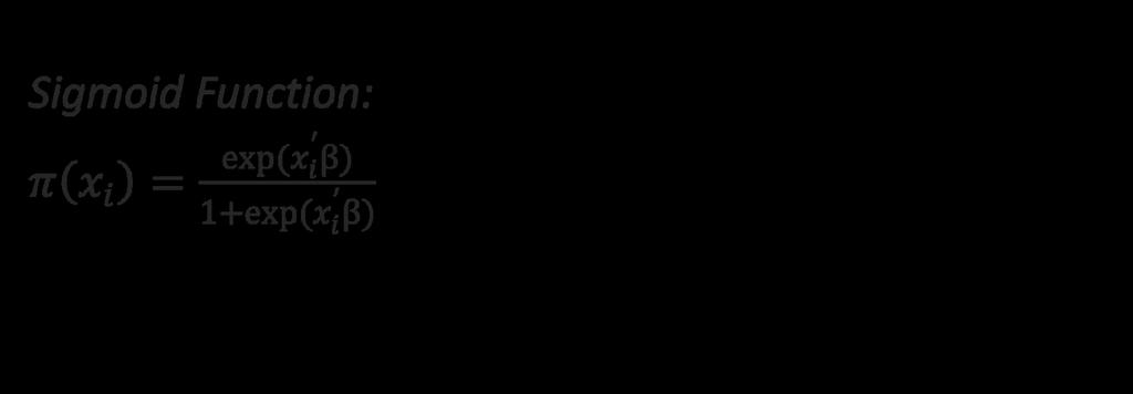
40 Binomial Data Allows for Logistic Regression 40

41 Methods One SNPs from 4K marker set was assigned to be QTN Taxa from the 282 diversity panel were simulated to experience lodging The 55K marker set was used to genotype the taxa used in the simulation 41

42 Objectives Evaluate the efficacy of the three model approach to mixed logistic regression Evaluate the use of the diversity panel for use in logistic regression GWAS Examine how variables within the data set effect the ability to detect a QTN 42

43 Simulation Study Settings Setting Grand Mean Stand Count Additive effect size

44 Model 1 identifies Peak SNPs While Accounting for Population Structure 44

45 45

46 What does changing the intercept do to our data?

47 Model 3 Failed to Converge in SAS Proc GLIMMIX Possible reasons for this failure: there was not enough variation in the response to attribute any variation to the random effect Estimated G matrix is not positive definite: procedure converged to a solutions where the variance of the random effect is 0 Alternative Solution: Use the GMMAT package (Chen et al. 2015) (Only runs on UNIX OS) 47

48 Model 2 Model 2 may have had enough power to successfully detect QTN despite model assumptions being violated Previous studies have shown that linear models can sometimes be approximated by logistic regression models 48

49 Conclusion Traditional GWAS requires normal data Logistic regression has the potential to analyze non-normally distributed traits The biggest limitation of using logistic regression is the computational power required Simulation Study show the need for increased variability of phenotypic data- this is especially hard to achieve in a binary trait 49

50 Model 1 identifies Peak SNPs While Accounting for Population Structure 50

51 Binomial Data Allows for Logistic Regression Logistic Regression does not require normality or equal variances Conduct GWAS by fitting a logistic regression model at each SNP Logit Link function: The natural log-odds of a plant is lodged or not lodged The grand mean

52 Model 2 Identifies Peak SNPs While Controlling for Population Structure and Relatedness Grand Mean Marker effect Random effects: account for familial relatedness Phenotype of i th individual Fixed effects: account for population structure Observed SNP alleles of i th individual Random error term Measures relatedness between individuals Yu et al. (2006) Adapted from A. Lipka 52

53 Model 3 is Fit Using Subset of Peak SNPs Model 3 is fit using top SNPs from Model 1 SAS 9.4 PROC GLIMMIX Recommendation: Number of SNPs that can be run in approximately 24 hours 53

54 Results of Simulation Study in Context of Stalk Lodging Data It is possible that our model s ability to accurately detect QTL was compromised because of an observed low rate of lodging Can we control If this baseline probability occurs, then the inability of our model to detect QTL may have been exacerbated by an intercept value that is far removed 0. 54

55 Peak SNPs that Coincide with Signals Associated with Related Traits Type of Region identified Chr Location in Literature Location in Model 3 Notes Marker Mb Mb Mb Mb Three most significant SNPs on Chr 7 qrpr2 QTL Mb Mb 14 th most significant SNP on Chr 2 qrpr3-1 QTL Mb Mb Mb 92 nd and 98 th most significant SNP On Chr 3 55