Insights into the Response of Rock Tunnels to Seismicity

Transcription

1 Master Thesis in Geosciences Insights into the Response of Rock Tunnels to Seismicity Mostafa Abokhalil

2

3 Insights into the Response of Rock Tunnels to Seismicity Mostafa Abokhalil Master Thesis in Geosciences Discipline: Environmental Geology and Geohazards Department of Geosciences Faculty of Mathematics and Natural Sciences UNIVERSITY OF OSLO [December 2007]

4 iv Mostafa Abokhalil, 2007 Tutor(s): kaare Høeg and Rajinder Kumar Bhasin This work is published digitally through DUO Digitale Utgivelser ved UiO It is also catalogued in BIBSYS ( All rights reserved. No part of this publication may be reproduced or transmitted, in any form or by any means, without permission. Cover photo: From the Norwegian newspaper VG ( )

5 v

6 vi Acknowledgment I would like to express my gratitude to Professor Kaare Høeg for being an outstanding advisor and excellent professor. I am indebted to Rajinder Kumar Bhasin for his supervision and his very useful and swift responds especially during the numerical modelling. Before I start this thesis, the time seemed very short and what was to be done seemed impossible to fit within the time resources. Their constant encouragement, support, and invaluable suggestions made this work successful within a short time. I would like to express my appreciation to the department of geosciences at the UIO for the facilities and my study place. I would like to extend my appreciation to the library staff that was very helpful and facilitated my research process, also the Norwegian Geotechnical Institute for lending me the software (Phase 2) and hosting many meetings. I am very grateful to my colleagues for helping me to keep on the road and never give up. The discussions with them were very useful. Finally, I owe a special gratitude to my family for their continuous and unconditional support during my thesis and through my life in general.

7 vii Abstract Underground structures are less sensitive to seismic shaking compared to surface structures. Several case histories reported damages to underground structures during major earthquake events. The damages are mainly related to the earthquake duration, seismic magnitude, and distance from the epicentre, ground behaviour, the depth, and the properties of the underground structure. The concepts of seismic design and modelling seismicity on tunnels excavated in rock masses were reviewed. Bhasin et al. (2006) conducted numerical experiments using Phase 2 version 5 which is a 2D elastic-plastic finite element stress analysis program for underground or surface excavations in rock or soil. They studied the seismic behaviour of rock support in circular lined tunnels excavated in weak and competent rock. Their research was verified and updated by using Phase 2 version 6. The verification included more representative factors in the analyses of the results. The software suitability in terms of numerical and theoretical procedures was investigated and found to be suited to the seismic simulations. The maximum axial force in the lining for tunnels in weak rock was found to increase 15% to 44% by Bhasin et al. (2006).In this thesis however it was updated to 19% to 38% after including the effect of rock support interaction. Numerical experiments were conducted to study the effects of seismicity on circular tunnels in rock masses with joints. The models were configured in a similar way to the earlier models by Bhasin and others in The effect of single joints and their orientation was simulated and studied in addition to two cases studies that include multiple joints. It was concluded that the competent rock deform along the joints. The maximum axial force in the lining occurs at the intersections between the joint and the tunnel lining. Neither the seismicity nor the orientation of the joint had a pronounced effect on tunnels in competent rocks with joints. Weak rock on the other hand may deform regardless of the locations of the joints and is affected clearly by seismicity. The maximum axial force in the tunnel lining does not occur necessarily at the intersections between the joints and the tunnel lining. Weak rocks were found to be less affected by seismic loads when they contain joints. The results were found to be in line with the Norwegian rock index system (Q system) guidelines and the earlier results by Bhasin et al. (2006).

8 viii

9 1 Table of contents 1. Introduction Background Purpose and Scope Case Histories and Lessons Learned Case histories The 1989 Loma Prieta earthquake The 1994 Northridge earthquake The 1995 Hyogoken-Nambu earthquake The 1999 Chi Chi earthquake The 1999 Duzce earthquake The 2004 Mid Niigata earthquake Main lessons learned from the case histories Seismic Design of Underground Structures Seismic design steps for underground structures Definition of seismic environment Evaluation of the ground response to shaking Assessment of structure behaviour due to seismic shaking Examples for seismic tunnel approaches Free field approach and a solution to ovaling deformations Pseudo-static analysis approach Modelling Seismic Effects on Tunnels in Rock Masses Construction of a representative model to simulate jointed rocks Phenomenological-type models... 21

10 Continuum-theory inspired models Generalized phenomenological models Numerical representation of joints Failure due to fatigue or cumulative displacements Joint orientation and spacing Bhasin et al. (2006) research on tunnels in rock without joints Suitability of the Phase 2 Program for Seismic Simulations Relevant numerical methods in rock mechanics Finite difference method and related methods Finite element method and related methods Boundary element method and related methods Distinct element method Hybrid models Suitability of Phase 2 numerical procedure Criterions for circular tunnel models Modelling ground behaviour Circular excavations models Suitability of Phase 2 criterions Numerical Analyses Performed Parametric study Configurations to the numerical simulations Effect of seismicity on tunnels in rock without joints Effect of seismicity on tunnels in rock with joints Case studies Case study 1: Effect of 2 parallel joints at Case study 2: Effect of multiple horizontal parallel joints... 52

11 3 7 Results of the Numerical Analyses Parametric study Effect of seismicity on tunnels in rock without joints Effect of seismicity on tunnels in rock with joints Case studies Case study 1: Effect of 2 parallel joints at Case study 2: Effect of multiple horizontal parallel joints Discussion of the Numerical Results Parametric study Effect of seismicity on tunnels in rock without joints Effect of seismicity on tunnels in rock with joints Case studies Case study 1: Effect of 2 parallel joints at Case study 2: Effect of multiple horizontal parallel joints Lessons learned from the case studies Conclusions and Recommendations Summary and Conclusions Applications and implications for practice Suggestions for future research References List of Figures Appendixes...90

12 4 1. Introduction 1.1 Background Designing underground structures to withstand seismic shaking did not receive proper attention in the past. In fact, the seismic design procedure was incorporated into a tunnel project for the first time only in the 1960s. The reason for this ignorance was the common belief among engineers that tunnels are invulnerable to earthquakes. However, some underground structures have experienced severe damages in the recent large earthquakes such as the 1995 Kobe, Japan earthquake, the 1999 Chi-Chi, Taiwan earthquake and the 1999 Kocaeli, Turkey earthquake. This gathered evidences have awakened the designers to the limitations of the above mentioned belief and led to a series of research studies. The philosophy of designing tunnels to withstand seismic loading is distinct from most surface structures. This is because of two main reasons. The first reason is that tunnels have inherent features that make their seismic behaviours different from most surface structures, mainly (1) their complete enclosure in soil or rock, and (2) their significant length. The second reason is that the seismic loads which cannot be calculated accurately unlike dead and live loads have also some specific features. They are superimposed, temporary, and cyclic. They are also derived with a degree of uncertainty. For most of the underground structures, the inertia of the surrounding soil/rock is large relative to the inertia of the structure. Thus the seismic response of a tunnel is dominated by the surrounding ground response and not the inertial properties of the tunnel itself (Bhasin et al., 2006). There are two methods to determine the seismic loads (1) the deterministic seismic hazard analysis (DSHA) and (2) the probabilistic seismic hazard analysis (PSHA). The later is the more recent and it explicitly quantifies the uncertainties in the analysis. It then develops a range of expected ground motions and their probabilities of occurrence. The probabilities can then be used to determine the level of seismic protection in a design (Hashash et al., 2001). However, the bottom line of designing tunnels generally relies on that they are less sensitive to seismic shaking than surface structures.

13 5 1.2 Purpose and Scope The purpose of this thesis is to provide insights into the behaviours of different rock supports in tunnels under the effect of seismic shaking. This thesis aims to achieve three goals; (1) it reviews the main advances in the field of seismic shaking effects on rock tunnels and (2), it conducts numerical experiments to update earlier research to determine the effects of seismic loading on competent rocks and weak rocks in tunnels. The earlier numerical simulations did not account for the rock support interaction whereas; it is included in computations in this thesis. (3) It performs new numerical experiments to study the effects of seismicity in the tunnels that suffer from the existence of planes of weakness. Similar models to the ones used in the earlier research were constructed and used in order to compare the results. Chapter 2 reports briefly the most recent cases for earthquake damages to underground structures then outlines the main lessons learned out of it. Chapter 3 outlines the three main steps to seismic design procedures. Chapter 4 reviews the earlier efforts in constructing models to simulate the effects of seismicity on underground structures. Chapter 5 investigates the reliability of Phase 2 which is the software used conduct the numerical simulations in this thesis. Chapter 6 describes the numerical analysis performed in this thesis. The chapter is divided into two parts. The first part presents a parametric study for the tunnels without joints and with singles joints that cross the tunnel in different orientations. The second part capitalizes on the findings from the parametric study through two case studies. The first case study is for two joints at a 45 and the second is for a set of multiple horizontal joints. Chapter 7 and chapter 8 present the results and discuss of the numerical simulations respectively. And finally chapter 9 presents the conclusions and recommendations. Several conclusions were found to be in line with the Norwegian tunnelling method (Q system).

14 6 2 Case Histories and Lessons Learned It is useful to briefly narrate the recent important case histories for underground structures that were hit by earthquakes. This emphasizes the significance of this research. The lessons learned are highlighted afterwards. Several studies have documented earthquake damages to underground structures. ASCE (1974) describes the damage in the Los Angeles area as a result of the 1971 San Fernando Earthquake. JSCE (1988) describes the performance of several underground structures, including an immersed tube tunnel during shaking in Japan. Other studies present summaries of case histories of damages such as; Duke and Leeds (1959), Stevens (1977), Dowding and Rozen (1978), Owen and Scholl (1981), Sharma and Judd(1991), Power et al.(1998) and Kaneshiro et al.(2000). Owen and Scholl (1981) have updated Dowding and Rozen s work with 127 case histories. Sharma and Judd (1991) generated an extensive database of seismic damage to underground structures using 192 case histories. Power et al. (1998) provide a further update with 217 case histories (Hashash et al., 2001).The following is a brief of some of the recent case histories. 2.1 Case histories The 1989 Loma Prieta earthquake The BART system is located on the San Francisco side and consists of underground stations and tunnels in fill and soft Bay Mud deposits, and is connected to Oakland via the transbay-immersed tube tunnel. During the 1989 Loma Prieta earthquake, the BART system experienced no damage and in fact, operated on a 24-h basis after the earthquake. This was primarily because the system was one of the first underground facilities to be designed with stringent considerations for seismic loading. The special seismic joints which were designed to accommodate differential movements maintained the functionality of the system. No damages were observed at these flexible joints, though it is not exactly known how far the joints moved during the earthquake (Hashash et al., 2001).

15 7 Another case was the Alameda tubes which are a pair of immersed-tube tunnels that connect Alameda Island to Oakland in San Francisco Bay Area. During the 1989 Loma Prieta earthquake the ventilation buildings experienced structural cracking, water leakage, and lose deposits above the tube at the Alameda portal. It is worth it to mention that the peak horizontal ground accelerations measured in the Area ranged between 0.1 and 0.25 g where g is the gravity. This underground facility was not designed with seismic considerations (Hashash et al., 2001) The 1994 Northridge earthquake The Los Angeles Metro was designed in several phases, some of which were operational during the 1994 Northridge earthquake. While the concrete lining in the bored tunnel remained intact, there were reported damages to the water pipelines, highways bridges and buildings. The horizontal peak ground accelerations measured near the tunnels ranged between 0.1 and 0.25g with vertical accelerations that is typically two thirds as large. The earthquake in this case did not cause the Metro system any damages (Hashash et al., 2001) The 1995 Hyogoken-Nambu earthquake The 1995 Hyogoken-Nambu earthquake caused a major collapse of the Daikai subway station in Kobe, Japan. This station represents the first modern underground structure to fail during an earthquake event. The design of the station did not take into account any seismic consideration. During the earthquake, shear walls at the ends of the station and at areas where the station changed width resisted the collapse of the structure. These walls suffered significant cracking. However the interior columns did not suffer as much damage. In the regions with no shear walls, the collapse of the centre columns caused the ceiling slab to crack. There was also significant separation at some construction joints, and corresponding water leakage through the cracks. The centre columns which were designed with very light shear reinforcement relative to the main bending reinforcement suffered damage ranging from cracking to complete collapse (Hashash et al., 2001).

16 The 1999 Chi Chi earthquake Several large highway tunnels excavated in rocky grounds were located within the zone heavily affected by the September 21, 1999 Chi Chi earthquake (ML 7.3) in central Taiwan. Most of the damages occurred at the tunnel portals because of slope instability triggered by the earthquake. Minor cracking was observed in the tunnel lining. No damage was reported in the Taipei subway, which is located over a 100 km from the ruptured fault zone (Hashash et al., 2001) The 1999 Duzce earthquake The Bolu tunnels are a 16-m-wide and 3.2-km-long twin tunnels and are part of the new Istanbul-Ankara highway. Their lines cross the North Anatolian Fault Zone (NAFZ). The tunnel is embedded in weak rock mass consisting of highly plastic clay which has poor strength. The extreme deformation due to the squeezing of this weak rook reached 720 mm near the opening of the tunnel.the 1999 Duzce earthquake (Mw=7.2) associated with the NAFZ caused a collapse within the portals (Kontogianni Villy and Stiros Stathis, 2003) The 2004 Mid Niigata earthquake The Joetsu Shinkansen s (bullet train) Uonuma tunnel which is 8625m long concrete tunnel constructed with the New Austrian Tunnelling Method crosses the Inokurayama fault. This fault was located just above the epicentre of the earthquake. The damage to the Uonuma tunnel is due to a possible activation of this fault. There was a large amount of leakage (200 l/min) during the construction time and an abrupt change in the geological layers. The leakage may have been connected to the river passing above the tunnel (Gazetas et al., 2005) Main lessons learned from the case histories The following are the main lessons learned from the case histories (Hashash et al., 2001): 1. Underground structures suffer less damage than surface structures 2. Reported damage decreases with increasing overburden depth. 3. Underground facilities constructed in soils and weak rocks suffer more damage compared to those which are constructed in competent rock.

17 9 4. The damage can be related to peak ground acceleration which is based on the earthquake magnitude and the distance from the epicentre. 5. The damages can be related to the duration of the earthquake because a longer earthquake may cause fatigue failure. 6. Damages at the near tunnel portals can be significantly attributed to slope instabilities.

18 10 3 Seismic Design of Underground Structures 3.1 Seismic design steps for underground structures This chapter is organized as it was suggested by the extensive literature review conducted by Hashash, Hook, Schmidt, and Yao in It explains the philosophy for designing tunnels and it emphasise the concepts employed in the numerical experiments performed later in this thesis as shown in Figure 3-1. Figure 3-1: Steps of Underground Structures Seismic Analysis and Design Procedure Modified after Hashash, Hook, Schmidt, and Yao in The following three steps were suggested to seismic design procedures for tunnels. 1- Definition of seismic environment 2- Evaluation of the ground response to shaking 3- Assessment of structure behaviour due to seismic shaking Figure 3-1 outlines the main three steps of underground Structures seismic analysis and design procedure suggested by Hashash, Hook, Schmidt, and Yao in 2001.However the figure was modified to show only the steps and not their extensive details in their review. The review is further adjusted and updated to focus mainly on the relevant topics for the thesis scope.

19 Definition of seismic environment Figure 3-2 shows the commonly identified types of seismic waves resulted from earthquakes. The most damaging type is the so-called Rayleigh waves which result from the compound effect of the primary waves and the secondary waves. In fact, one reason for the less vulnerability of underground structures is because Rayleigh waves decay exponentially with depth and become negligible when down to 15-20m (Singh, Goel 2006). The response of rock tunnels to seismic waves is expressed by their deformations. For simplicity, these deformations are assumed usually to be identical to the deformations of the surrounding rock mass (Kolymbas 2005). In order to identify the ground motion parameters for example velocities and accelerations, one must conduct the so called deterministic seismic hazard analysis (DSHA) and/or the probabilistic seismic hazard analysis (PSHA). After the DSHA and/or the PSHA have identified the level of shaking at the site, it becomes possible to identify the parameters needed for the engineering design. The choice of these parameters depends on the design method. At a particular point in the ground or on a structure, ground motions can be described by three translational components and three rotational components. The components of ground motion can be characterized by acceleration, velocity or displacement coupled with three significant parameters; amplitude, frequency and duration (Hashash et al., 2001). Research has shown that transverse shear waves transmit the greatest proportion of the earthquake s energy. The amplitudes in the vertical plane have been typically estimated to be a half to two-thirds as great as those in the horizontal plane. However, in recent earthquakes such as 1994 Northridge and 1995 Hyogoken-Nambu, measured vertical accelerations were equal to and sometimes larger than horizontal accelerations (Hashash et al., 2001).

20 12 Figure 3-2: Typical types of different seismic waves resulting from earthquakes modified after the west publishing company (1995) Evaluation of the ground response to shaking Ground response to shaking may vary between failure to no or limited damages. Ground failure as a result of seismic shaking includes liquefaction, slope instability, and fault displacement. Ground failure is particularly prevalent at tunnel portals and in shallow tunnels.

21 13 Liquefaction is a term associated with a host of different, but related phenomena. It is used to describe the phenomena associated with increase of pore water pressure and reduction in effective stresses in saturated Cohesionless soils the rise in pore pressure can result in generation of sand boils, loss of shear strength, Lateral spreading and slope failure. Slope instability results in landslides which affects mostly the tunnel portals. In this case, the primary failure mode tends to be slope failures (Hashash et al., 2001). Fault displacement cause severe damages to underground structures. It is not always possible to avoid crossing a fault zone. If the design of the underground structure does not accommodate the resulting displacements, serious damages may occur. The case of the railway tunnel crossing the White Wolf Fault (WWF) is an example. The tunnel was seriously damaged during the 1952 Kern County earthquake (Mw=7.5) associated with this fault. Luckily for Norway and North West Europe in general, the tunnels are not highly vulnerable to seismic shaking. This is because these areas are identified as tectonically inactive areas (Kontogianni Villy and Stiros Stathis, 2003). This thesis examines rock tunnels in particular. Subaqueous tunnels, immersed, soft ground tunnels and tunnels bored through soil grounds are not the main interest in the scope of this work. For rock tunnels, Ground shaking and deformation will be the most expected behaviour during and after earthquake event. Figure 3-3 shows the typical cross section of tunnels. The major factors influencing shaking damage include: 1. the shape, dimensions and depth of the structure; 2. the properties of the surrounding soil or rock; 3. the properties of the structure; and 4. the severity of the ground shaking (Hashash et al., 2001). The design of tunnels to accommodate seismicity differs from the design of surface structures. While surface structures are not dominated by the inertia of the ground, rock tunnels are dominated by the properties and the response of the surrounding ground. Therefore, it is usually represented by an elastic beam subject to deformations induced by the surrounding medium. Axial deformations in tunnels are caused by the parallel components of seismic waves to the axis of the tunnel which alternates between compression and tension.

22 14 Figure 3-3: Typical cross section of tunnels (Hashash et al., 2001).

23 15 Figure 3-4: Effects of deformations of tunnels due to the seismic shaking (Hashash et al., 2001).

24 16 The response of tunnels to seismic motions can be categorized into three types which are shown in the figure 3.4 where, (1) Axial compression and extension, (2) longitudinal bending (3) ovaling/racking (Bhasin et al., 2006). Longitudinal Bending deformations are caused by the perpendicular components of seismic waves to the longitudinal axis of the tunnel. Ovaling or racking deformations are caused by shear waves propagating normal or nearly normal to the tunnel axis (Hashash et al., 2001) Assessment of structure behaviour due to seismic shaking The assessment of seismic design is based on two main concepts; the maximum design earthquake (MDE) and the operating design earthquake (ODE). In the deterministic seismic hazard analysis (DSHA) the MDE is the maximum level of shaking that can be experienced at the site, while in the probabilistic seismic hazard analysis (PSHA) the MDE is defined as an event with a small probability of exceedance (2-3%) during the life of the structure. In risk analysis studies it is commonly acknowledged that the risk equals the hazard times the consequence (R= H C). This is why the MDE design goal is to secure only the public safety during and after the earthquake event and allows controlled damages for the structure. The design loads for the MDE are a product of the worst scenario of load combinations. The operating design earthquake (ODE) is an earthquake event that can be reasonably expected to occur at least once during the design life of the structure. In the probabilistic seismic hazard analysis (PSHA) this is coupled with probability of exceedance between 40 and 50%. The ODE design goal is that the overall system shall continue operating during and after an ODE. In this design criterion a little or no damage is allowed. Inelastic deformations must be kept to a minimum meaning that the response of the underground facility should therefore remain within the elastic range (Hashash et al., 2001) There are several engineering approaches to compute the deformations and forces induced by seismic waves. These deformations depend on the type of ground, the type of structure and, the interaction between the ground structure interactions.

25 Examples for seismic tunnel approaches The simplest approach is the free-field ground deformations. In this approach the interaction of the underground structure with the surrounding ground is ignored. The deformations due to a seismic event are then estimated, and the underground structure is designed to accommodate these deformations. This approach is satisfactory when low levels of shaking are anticipated or the underground facility is in a stiff medium such as rock. In the dynamic analysis approach, a dynamic soil structure interaction is conducted using numerical analysis tools such as finite element or finite difference methods. In the pseudo-static analysis approach, the ground deformations are imposed as a static load and the soil-structure interaction does not include dynamic or wave propagation effects (Hashash et al., 2001). However, it is important to understand the hypothesis of these approaches. The pseudo-static approach is incorporated in the software tool Phases 2 which is used to compute the numerical simulations later in this thesis. The analytical solutions of ovaling deformations of circular tunnels the pseudo- static theory and it is practical application are briefly discussed in the following text Free field approach and a solution to ovaling deformations This type of deformation occurs only for circular tunnel cross sections. The circular shape is going to be the subject of the numerical simulations conducted later in this thesis. The simplest form to estimate ovaling deformations is to neglect the effect of soil-structure. This assumption is reasonable when the ovaling stiffness of the lined tunnel is equal to the surrounding ground. In other words the model assumes that there is no tunnel (referred as non-perforated ground) as shown in figure 3-5. The diametric strain for a circular section is calculated as: dd ffffffff ffffffffff dd = ± γγγγγγγγ 22 Equation 3-1 Where:

26 18 d free-field: Free field diametric deflection in non-perforated ground d: diameter or equivalent diameter of tunnel lining γ max: maximum free-field shear strain of soil or rock medium If the ovaling tunnel stiffness is very small compared to the surrounding ground, the model of perforated ground is invoked. This will lead to adjusting the equation to: dd ffffffff ffffffffff dd = ±2γγγγγγ xx(1 νννν) Equation 3-2 Where ν m: the Poisson s ratio of soil or rock medium The deformations induced in this case are clearly more that the pervious case. The lining interaction with the ground has to be taken into account in most cases. To do so, the relative stiffness of tunnel is first quantified by the compressibility and flexibility ratios (C and F) which are given by the following equations CC = 2 EEEE (1 νν 1)rr EEEE.tt(1+νννν )(1 2νννν ) Equation 3-3 FF = EEEE (1 νν 2 1)rr 3 6EEEE.II(II+νννν ) Equation 3-4 Where: C: compressibility ratio of tunnel lining E m : modulus of elasticity of soil or rock medium ν 1 : Poisson s ratio of tunnel lining t: thickness of tunnel lining I: moment of inertia of the tunnel lining (per unit width) for circular lining F: flexibility ratio of tunnel lining r: radius of circular tunnel Figure 3-5: Tunnel in a free field shear strain (Hashash et al., 2005).

27 19 In 2005, Hashash and others updated the analytical solutions for estimating the ovaling deformations and forces in circular tunnels due to soil-structure interaction under seismic loading (Hashash et al., 2005). There are two analytical solutions available: (1) Wang (1993) and (2) Penzien (2000). Wang (1993) reformulated the above mentioned equations to adapt to the seismic loading caused by shear waves. The free field shear stresses were replaced by in-situ overburden pressure and the at rest of the coefficients of earth pressure is assigned a value of (-1) to simulate simple shear condition. The shear stress is later expressed as a function of shear strain. The solution will handle three cases (1) thrust (full-slip, no-slip), (2) shear and (3) moment in the tunnel lining. Penzein (2000) developed similar analytical solutions. However, a comparison with the numerical analysis discovered that Penzien (2000) solutions significantly underestimates the thrust in the tunnel lining for the condition of no-slip and therefore should not be used for this condition(hashash et al., 2005) Pseudo-static analysis approach The analysis of seismic response may be approached by many methods such as static approach, pseudo-static approach, and dynamic approach. The pseudo-static approach has gained more popularity in geotechnical engineering because it is neither simple like the static nor complex and time consuming like the dynamic. It is also being used by the software which will compute the later numerical simulations in this thesis. This approach assumes as shown in the figure 3-6 that the unit weight of rock mass (γ) is modified to ((1+αv).γ) to represent the seismic loads. An approximate estimation of the increase in the support pressure is as follows In the roof P (seismic) = (αv). P (roof) Equation 3-5

28 20 In the walls P (seismic) = (αh). P (wall) Equation 3-6 Where P (seismic), P (roof), P (walls) are the earthquake, static pressure in the roof and the static pressure in the walls sequentially. The coefficients of vertical (αv) and horizontal acceleration (αh) are approximated to (0.25). This approach constitutes the basis for seismic design of rock tunnels in NGI quality index system (Q) which is given by the following formula: Q (seismic) QQ (1 + αα) 3 QQ 2 Equation 3-7 In other words: Q (seismic) 1 RRRRRR 2 Q (static) JJJJ JJJJ JJJJ JJJJ 2(SSSSSS) (Barton, 1984) Equation 3-8 The above equation suggests a 25% increase in rock support pressure according to the charts of the Q system (Singh, Goel 2006). Rushan and Hongbin (2006) improved a Pseudostatic method for a simple boxed-tunnel shape embedded one- dimensional soil layer. One of the key improvements in their method is to include the effect of soil damping. They found that the Figure 3-6: Seismic loads on a tunnel soil damping is responsible for the deviation in the results from the dynamic analysis. The Improved Pseudo static method consists of two main steps: The first is using one-dimensional seismic response analysis program to conduct the seismic free field analysis. Secondly is to conduct the pseudo- static approach with the help of numerical modelling tools. They did not apply the method on rock tunnels but they argue that their method may be applicable for any complex soil condition (Rushan and Hongbin, 2006).

29 21 4 Modelling Seismic Effects on Tunnels in Rock Masses One of the main goals of this thesis is to investigate the effects of seismicity on tunnels excavated in rocks with and without joints. Later in this thesis models for single and multiple joints crossing and intersecting with the tunnel lining were simulated. This chapter discuss briefly the state of the art regarding the aspects of modelling seismicity on rocks with and without joints. When dealing with underground structures, the main aspects of concern regarding joints are the following: 1. Construction of a representative model to simulate jointed rocks 2. Failure due to fatigue or cumulative displacements 3. Joint orientation and spacing The above mentioned aspects will be discussed in this chapter in the same order.in the last section, Bhasin and others research on tunnels in rocks without joints will be presented in more detail. The numerical simulations that were conducted by Bhasin and others in 2006 were replicated and the results were verified once again. The figures presented in this section are similar to those presented in their research. This is the only part in the thesis where the author of this thesis used Phase 2 version 5 instead of version 6 to replicate the earlier research. 4.1 Construction of a representative model to simulate jointed rocks The following are the main types of the physical models used to represent rock joints Phenomenological-type models Those are the types of models that are produced in order to match or explain a phenomenon in the field. In practice, the loading conditions are more complicated than those used in these

30 22 models. As an example, Heuze and Barbour (1982) developed a model to reproduce peak Shear stress measurements under constant normal load (CNL) and constant normal stiffness (CNS). This model assumes that the joint dilates immediately upon shear displacement. This means that the dilation angle is assumed to be constant just until the joint fails then after this point it drops to zero instantaneously(morris, 2003) Continuum-theory inspired models These models are built upon the continuum treatments of rock mechanics. Morris ( 2003) argues that the theoretical base of these models are solid, But that it is difficult to relate the variables and parameters used by such models to the results of specific experiments. As an example, Nguyen and Selvadurai (1998) suggested a model to account for hydraulic behavior in rock joints. In this model before the yield, the joint response is elastic. When yielding, the displacement on the joint has elastic and plastic components. These plastic components of displacement can include dilatant effects. The plastic deformation leads to degradation of the joint asperities and a reduction in friction angle (Morris, 2003) Generalized phenomenological models This type of model combines the spirit of the phenomenological-type models and the continuumtheory inspired models mentioned earlier. They are less complicated than the continuum-theory inspired models. As example for those models is the Itasca s 3DEC models which employ the concept of plastic deformation (Morris, 2003) Numerical representation of joints The mechanical behaviour of a jointed rock mass is difficult to model because of the complexity of discontinuities. This complexity is due the difficulty to represent the jointed rock mass geometrically and behaviourally. Therefore, it is well recognized that there are severe limitations on the applicability of the empirical relationships. Those empirical relationships such as Hoek- Brown strength criterion are the basis for the output of numerical models. The following are the four approaches often adopted in rock mechanics (Lin and Ku, 2006).

31 23 1. The equivalent continuum approach which modifies the rock constitutive law to include the mechanical effects of joints that are dense and follow a regular pattern. 2. The continuum with joint interface approach which introduces discontinuous interfaces to model each joint in a rock mass. This approach is simple to implement into finite elements but its application is limited to cases where the geometry does not undergo substantial changes. 3. The discrete element approach which models the kinematics across each joint explicitly. This is a powerful tool if a rock mass is delimited into blocks by joints. 4. The discrete continuum approach which encompasses the strength of both the continuum and the discrete approach. Recent advances in discontinuity modelling provide an opportunity for two-scale modelling. 4.2 Failure due to fatigue or cumulative displacements As discussed before, there is gathered evidence that underground structures suffer less damage compared to surface structures under an earthquake event. However, there are other types of seismicity that affect only underground structures for example; mining -induced seismicity and explosions. Peak particle velocity (PPV) in a ground wave is usually one of the accepted representative parameters for defining dynamic design loads. One concept for expressing damages in underground structures is to relate the PPV to the extent of damage. So if the PPV at a site is smaller than the threshold value, then no damages are to be expected (Ma and Brady, 1999). It is recognized that joint deformation is a critical aspect of the response to dynamic loading of excavations in jointed rock. Under cyclic shear loading, joint deformation increases and joint shear strength decreases. Catastrophic failure occurs when the accumulation of deformation is such that the residual strength locus is intercepted. St John and Zahrah (1987) proposed that under dynamic loading, damage to an excavation is determined by the number of excursions of joint motion into the range of plastic constitutive behaviour (Ma and Brady, 1999).

32 24 Ma and Brandy (1999) conducted a numerical study to investigate the dynamic performance of an underground excavation in jointed rock subject to repeated seismic loading. They used the Universal Distinct Element Code to perform the numerical simulation. They simulated the field situation for Lucky Friday mine in Mullan-Idaho- USA and compared their results with the observations collected from the field. In that case of Lucky Friday mine, the seismicity was induced by slip on structural features in the stress field caused by mining. Ma and Brandy (1999) discussed the differences in the results when using the dilation angle in two criterions namely the Mohr-Coulomb and the continually yielding. The figure bellow shows the model geometry for the site. Figure 4-1: Model geometry for Lucky Friday mine in Mullan-Idaho- USA site (Ma and Brady, 1999). They compared the results of the cumulative joint displacements and proposed that the continuously yielding joint model better produces the observed results than the Mohr Coulomb joint model. They concluded that, in rock masses subject to repeated dynamic loading,

33 25 excavation design may need to account for the prospect of repeated episodes of transient loading at the excavation site (Ma and Brady, 1999). Their study stressed the effects of repeated seismic loading in terms of the cumulative joint displacements because after a threshold point failure is expected. The jointed model of their simulation was complicated but was backed by the historical data collected from the field. 4.3 Joint orientation and spacing Tunnels in jointed rocks are affected by the joint orientation during the excavation process and after construction. During the excavation the favourable joint orientation will affect the excavation process positively. The performance of tunnel boring machines (TBM) is highly dependent on the fragmentation efficiency of its cutters. The efficiency of those cutters is related closely to the joints orientation. This is because the joint orientation affects the crack initiation and propagation as well as the fragmentation pattern. The cutter penetration in the TBM may be affected by two angles: the angle α between the tunnel axis and the joint plane, and the attack angle ß between the cutter rolling direction and the joint outcrop in the tunnel face (Gong et al., 2005). However, a detailed illustration is not the main focus of this thesis. Figure 4-2 shows the influence of joint orientation on TBM penetration. Tunnels in jointed rocks can be subjected to severe dynamic loads due to rock bursts, coal bumps and large earthquakes. The effects of joint orientation in such cases Figure 4-2: Influence of joint orientation on TBM penetration (Gong et al., 2005).

34 26 were modelled by Heuze (2004). He used a series of 3-dimensional simulations based on discrete element analysis namely the LDEC 3-dimensional discrete element code. He configured two rock-island configurations and described his models as follows The rock island is 16mx16mx1m. The tunnel is 4-m wide by 5-m high. The rock joint spacing is 0.7m in the plane of the figure and there is one block in the thickness of the island. The simulations were performed in plane strain He concluded that joint orientation has a significant effect on the tunnel hardness. He compared between two models where he changed the angles of the joints orientation. The tunnel stability was greatly enhanced when the joint dip angles was reduced which is an acknowledged field observation (Heuze, 2004). In another study, the stability of underground openings excavated in a blocky rock mass was studied using the discontinuous deformation analysis (DDA) method. The research focused on kinematical analysis of the rock deformation as a function of joint spacing and friction. It has been concluded that the joint orientation is an important factor in the stability. Different geometries were used for the excavations and the geometries were found to have different states of stabilities (Tsesarsky and Hatzor, 2006) Joints spacing was also investigated by Heuze (2004) in his previously mentioned models. He found that when reducing the joint spacing from 70cm to 35 cm, the tunnel stability was dramatically affected. Reducing the joint spacing will decrease the stability of the tunnel (Heuze, 2004). Notice that Heuze (2004) performed many simulations for underground openings in jointed rocks. He used the discontinuous deformation analysis (DDA) method to conduct his simulations. The geometries that he studied were for complicated sets of joints. When Ma and Brandy (1999) conducted a numerical study to investigate the dynamic performance of an underground excavation in jointed rock subject to repeated seismic loading, they used the Universal Distinct Element Code to perform the numerical simulation. The geometry for their model was also complicated.

35 Bhasin et al. (2006) research on tunnels in rock without joints The following is a literature coupled with verification of its results. All the experiments were verified solely to cross check the results and the findings. The reason for this is that, these numerical experiments are further built upon to construct the models used in the rest of the numerical simulations in the thesis. An earlier research took place in a joint cooperation between the Norwegian Geotechnical Institute (NGI) and the Indian institute of technology Roorkee by Bhasin and others. The research results were published on the 13 th symposium on earthquake engineering in The methodology was based on a series of numerical simulations using 2D finite element programme Phase2, version 5 (2004) and the research aimed to investigate the effect of seismicity on tunnel lining in tunnels of different sizes. Both linearly elastic and elastic-plastic analyses were performed. The elastic material in the elastic model was defined as not to undergo a progressive failure such as in weak rocks whereas, in the plastic analysis the material was defined as elasticperfectly plastic in which no brittle failure can occur (Bhasin et al., 2006). In the numerical simulations the overburden was kept constant for all the models. That is, 60 meters above the roof of all the circular tunnels. The size of the tunnels varied from 5 to 20 m in diameter. For simplicity, the tunnels were assumed to be dug on two stages. In stage one the excavation took place and in stage two a tunnel lining of 0.1m thick shotcrete was applied. The time between the completions of stages one and two was assumed to be short enough not to allow for deformations in the tunnel. The models were run to equilibrium in both the linear elastic (competent rock) and elastic perfectly-plastic (weak rock) cases considering only the static loads at first then, the seismic loads were superimposed. The seismic loading was superimposed as quasi-static and in different directions. For all the model simulations the following multiple analyses were performed: 1- Seismic coefficient in the horizontal direction; h= Seismic coefficient in the vertical direction; v= Seismic coefficients in both the horizontal and vertical direction; h=0.3 and v=0.2

36 28 Figure 4-3: Static loading in a 10m diameter tunnel in elastic rock. Fig 4-3 shows the case of a static loading in a 10m diameter tunnel in an elastic rock. Figure4-4 shows an elastic analysis plot for a 10 m diameter tunnel when the horizontal seismic coefficient is 0.3. In this case the maximum axial force on the lining is MN which is almost the same as that in static loading conditions in elastic analysis. However, there has been a redistribution of forces along the periphery of the lining after the application of peak horizontal acceleration, though the maximum axial force remains the same for both static and dynamic loading conditions. Figure 4-5 shows a corresponding plastic analysis plot for a 10 m diameter tunnel. In this case the maximum axial force on the lining is MN which is much higher than in the elastic analysis Figures 4-6 and 4-7 show respectively the elastic and plastic analyses. This is shown when the vertical seismic coefficient is 0.3. It can be seen that the maximum axial force on the lining is higher for the plastic analysis (0.941 MN) than for the elastic analysis (0.346 MN).

37 29 Figure 4-4: Elastic analysis plot for a 10 m diameter tunnel when the horizontal seismic coefficient is 0.3. Figure 4-5: Plastic analysis plot for a 10 m diameter tunnel when the horizontal seismic coefficient is 0.3. Figure 4-6: Elastic analyses for a 10 m diameter when the vertical seismic coefficient is 0.3.

38 30 Figure 4-7: Plastic analyses for a 10 m diameter when the vertical seismic coefficient is 0.3. Figures 4-8 and 4-9 show respectively the maximum axial force on the lining for the elastic and the plastic analysis. It shows the analysis when both the horizontal and vertical seismic coefficients are applied. Once again it can be seen that the maximum axial force on the lining is much higher for the plastic analysis than for the elastic analysis. Figure 4-8: Elastic analyses for a 10 m diameter when both the vertical seismic coefficient and the horizontal are applied.

39 31 Figure 4-9: Plastic analyses for a 10 m diameter when both the vertical seismic coefficient and the horizontal are applied. Similar elastic and plastic analysis studies were performed for tunnels of different sizes and the results are summarised in table 1. Figure 4-10 compare and summarize the results also between the elastic and the elastic-perfectly plastic rocks. It can be seen from this figure that for the elastic analysis there is not much difference in the maximum axial force on the lining as the tunnel dimension increases from 5 to 20 m. In addition there is not much difference in the maximum axial force on the lining when dynamic loading is applied as compared to static loading. For plastic analysis the load on the lining increases significantly with the tunnel diameter when dynamic loading is applied. Furthermore, there is a significant increase in the maximum axial force when dynamic loading is applied as compared to static loading. Table 1: Summary of the numerical results Seismic loading Static loading on Static loading on Seismic loading h=0.3& h=0.3& v=-0.2 on strong rock weak rock v=-0.2 on strong rock weak rock D diameter Max. Axial Force Max. Axial Force Max. Axial Force Max. Axial Force %increase of MAFL in the weak Rock

40 32 Max Axial force on the tunnel lining MN summary of the numerical results Tunnel diamater (m) Static loading on competnet rock Static loading on weak rock Seismic loading h=0.3& v=-0.2 on competent rock Seismic loading h=0.3& v=-0.2 on weak rock Figure 4-10: Summary and of the results and a comparison between the weak and competent rock The following points are the main outcomes of the pervious experiments: 1- For elastic rock (competent rock), there is no significant difference in the Maximum axial force in the lining (MAFL) between static loading and after superimposing the seismic loading. 2- For elastic -perfectly plastic rock (weak rock), there is a significant difference between the static loading and after superimposing the seismic loads in the (MAFL). 3- For elastic rocks, there is no significant effect for changing the size of the tunnel on the (MAFL). 4- For elastic -perfectly plastic rock, as the size increases the (MAFL) increases significantly. 5- It was also shown that for the weak rock mass the difference in the axial force on the lining ranges from 15% to 44% between the static and dynamic loading. In the opinion of researchers who conducted this research, this complies with the Q-system suggestion of 25% increase in the support pressure to account for the seismic forces (Bhasin et al., 2006).

41 33 5 Suitability of the Phase 2 Program for Seismic Simulations The method of performing research in this short thesis was mainly based on bibliographic, internet research and the simulations run in Phase 2 version 6 (2006). The following journals were very useful ; Tunnelling and underground space technology, International journal of rock mechanics &Mining sciences, Soil dynamics and earthquake engineering, structural design, and earthquake engineering and other journals. Phase 2 version 6 (2006) is a 2D elastic-plastic finite element stress analysis program for underground or surface excavations in rock or soil. This software offers to employ the following criterions; Mohr-coulomb, Hoek-Brown, Drucker-Prager and Generalized Hoek-Brown for plastic modelling. If no criterion was chosen the model will assume an elastic model. Discontinuities can only be introduced by adding joints. Joints can be defined by joint normal stiffness and shear joint stiffness. One can choose between Mohr-coulomb and Barton-Bandis for a slip criterion in rock joints. In this chapter Phase 2 will be examined in terms of theory and numerical analysis. The aim is to justify its validity to the research problems in this thesis. The relevant numerical analysis models are discussed in the first section followed by a judgement on the suitability of phase 2. In the second section, the criterions for circular excavation models are discussed followed by a judgment on the suitability of phase Relevant numerical methods in rock mechanics There are a variety of rock mechanical modelling methods. These methods can be classified in different manners. One way of classifying them is to group them under four main categories as follows (Jing and Hudson, 2002) A. Methods based on previous experience B. Methods based on simplified models C. Methods based on modelling which attempts to capture most relevant mechanisms D. Methods based on all- encompassing modelling

42 34 Figure 5-1: The four basic methods, two levels, and hence eight different approaches to rock mechanics modeling and providing a predictive capability for rock engineering design(jing and Hudson, 2002). The figure above illustrates the classification which was proposed by Jing and Hudson in They explain it as follows Level 1, includes methods in which there is an attempt to achieve one-to-one mechanism mapping in the model. In other words, a mechanism which is thought to be occurring in the rock reality and which is to be included in the model is modelled directly, such as an explicit stress strain relation Level 2, includes methods in which such mechanism mapping is not totally direct, e.g. the use of rock mass classification systems. Some of the rock mass characterization parameters will be obtained from site investigation, the left-hand box. Then the rock engineering design and construction proceeds, with feedback loops to the modelling from construction

43 35 The most commonly applied numerical methods for rock mechanics fall in the following three categories (Jing and Hudson, 2002). (Notice that the above mentioned classification was for the modelling methods in general but now it is the numerical methods specifically which are to be classified). 1. Continuum methods the finite difference method (FDM), the finite element method (FEM), and the boundary element method (BEM). 2. Discrete methods the discrete element method (DEM), discrete fractures network (DFN) methods. 3. Hybrid continuum/discrete methods. The choice of the method depends on the problem under research. The continuum methods can be used when few fractures are present in the rock mass under modelling. The discrete methods are used for moderately fractured rock. If the rock contains a large number of fractures, then hybrid methods are used (Jing and Hudson, 2002) Finite difference method and related methods The basic technique in the finite difference method FDM is the discretization of the governing partial difference equations (PDEs). This is by replacing the partial derivations with differences defined at neighbouring grid points. There is no need for a global system of equations in a matrix form in the FDM. After the replacing of the partial derivations with differences, the solutions of the equations become localized. This is a very useful advantage because it reduces the storage and the memory requirements needed from the computer. Also the PDEs are not approximated in the FDM which means that there are no iterative solutions. This allows for simulating difficult behaviours such as plastic behaviour of rocks in a very straight and fast manner (Jing and Hudson, 2002). The disadvantages in this method are due to that it cannot deal properly with fractures, complex boundary conditions and material heterogeneity. These disadvantages tie the applicability of the FDM in many important problems in rock mechanics. However, the ability of the FDM to deal with irregular meshing and material heterogeneity can be enhanced greatly through the so called

44 36 finite volume method FVM. A well-known computer code that uses the FDM coupled with FVM is the FLAC code group. Even after coupling FDM with FWM, it still becomes not easy to explicitly represent fractures. Therefore this defect remains as the main disadvantage of this Method (Jing and Hudson, 2002) Finite element method and related methods The finite element method (FEM) is probably the most applied numerical method in rock mechanics. Before using the FVM to enhance the flexibility of the ordinary FDM, the FEM had a clear advantage because of its flexibility to treat material heterogeneity, non-linear deformability, complex boundary conditions, in situ stresses and gravity. However, the treatment of fractures and fracture growth remained the most important limitation for this method. This is because of the global stiffness matrix becomes ill-conditioned after introducing multiple fractures in the continuum. It is also not possible to treat problems of block rotations and large scale fractures openings. The FEM cannot treat fracture growth problems because it is limited to a small element size and the need for continues re-meshing with the fracture growth. This shortcoming in the FEM led to the development of the so called bifurcation theory, enriched FEM and generalized FEM. Those techniques use discontinues shape functions for implicit simulations of the crack initiation and fracture growth problems. The meshes can be independent of the problem geometry (Jing and Hudson, 2002). There is also another type of shortcoming in FDM regarding it is meshing. The ordainary FDM cannot deal with complex interior and exterior boundaries. This shortcoming can be fixed by using the so called element-free methods. These are methods to simplify the meshing process and can represent complex boundaries. However, one element remains the main powerful side in FDM in general which its computational power. It provides high accuracy(jing and Hudson, 2002) Boundary element method and related methods The boundary element method BEM employs a different procedure when compared to the FDM and the FEM. It seeks a weak solution initially and then improves it later. This method has been

45 37 used successfully to solve different problems such as; the general analysis for the stresses and deformations around underground excavations, soil structure interaction applications, ground water flow and fracturing processes (Jing and Hudson, 2002). One of the main advantages of the BEM is that it reduces the model dimensions. This advantage made the method very suitable to simulate the 3-D applications. There are two related methods used with this method to simulate the fracture growth problems and to simulate the stresses. These methods are namely and sequentially, the displacement discontinuity method (DDM) and the fictitious stress method(jing and Hudson, 2002). The BEM can simulate with simplicity the 3-D problems unlike the traditional the FDM and the FEM. However, it is not an efficient method to deal with material heterogeneity such as the FEM. It is also efficient to simulate the non-linear material behaviour such as plasticity. The BEM is suitable for simulating fracturing in homogenous elastic bodies (Jing and Hudson, 2002) Distinct element method The concept of the distinct element method (DEM) was originally used to solve problems in rock mechanics. The DEM treats the domain of interest in the problem in a unique way. It represents the domain by assemblage of rigid and deformable blocks or particles. The contact among those rigid and deformable blocks are updated continuously and represented during the deformation process. The theoretical foundation of the method is the formulation and solution of equations of motion of rigid and/or deformable bodies using implicit (based on FEM discretization) and explicit (using FDM/FVM discretization) formulations. In fact this is the main difference between the DEM and the continuum-based methods. The previously mentioned continuumbased methods lack the ability to update and continuously change the boundaries during the deformation process. The most common DEM codes are the UDEC and 3DEC computer codes which handle two and three dimensional problems (Jing and Hudson, 2002). The DEM is suitable to a very wide range of applications in rock mechanics. It also has been expanded to deal with granular materials for geo-mechanics and rock engineering. The PFC

46 38 codes for both two and three dimensional problems also the DMC codes are popular in this field. Actually, the DEM has been applied in many other fields such as soil mechanics, the processing industry and defence research (Jing and Hudson, 2002). The method is implicitly incorporated in the so called, the discontinuous deformation analysis (DDA) approach which is a tool to analyze stress deformations. The DEM uses the standard FEM meshes over blocks. The contacts between those blocks are dealt with using the so called penalty method. There are similar approaches in the field of numerical methods such as; the discrete finite element method and the combined finite discrete element method. However the DDA comes in the first position in terms of development. The DDA uses larger time steps that the ordinary DEM and can accept easily transformations from other codes such as FEM codes (Jing and Hudson, 2002) Hybrid models The so called hybrid models are frequently used in rock engineering, and basically for flow and stress deformation problems in fractured rocks. The main hybrid combinations are BEM/FEM, DEM/FEM and DEM/BEM. In the case of the hybrid BEM/FEM, the BEM is used to simulate the far field rocks as an equivalent elastic continuum and the FEM to simulate the near field nonlinear behaviours. This provides more effective simulations of the far field and the near field rock masses. The Hybrid FEM/BEM is a common hybrid and is used mainly for simulating the mechanical behaviours of underground excavation and the hybrid DEM/BEM model is used mainly to deal with stress/deformation analysis(jing and Hudson, 2002). The hybrid models are clearly advantageous compared to the single methods because it deals with the domains in a more specific manner. Thus, it employs the appropriate method for each part in the problem Suitability of Phase 2 numerical procedure The above mentioned methods are just those which are commonly used to deal with underground excavations in rock mechanics and also within the domain of our research questions. Popular methods like the inverse solution methods or the neural networks are not illustrated here because

47 39 they are irrelevant to this research. However, an extensive review of these methods is found in Jing, L. paper A review of techniques, advances and outstanding issues in numerical modelling for rock mechanics and rock engineering (Jing, 2003). The main reason we went through the trouble of presenting the above motioned numerical methods was to evaluate the objectivity of using our modelling software. As stated by Phase 2 developers, it is a 2D elasto-plastic finite element stress analysis program for underground or surface excavations in rock or soil. This means that it enjoys all the ordinary FEM properties but also suffers also from its shortcomings. But this suits our research problems well, because our models contain no fractures. The parameter study and the case studies presented in this thesis later require the representation of the plastic behaviour of rock masses. If Phase 2 program for example had the BEM in its calculation system, then the software should not be suitable methodologically for simulating the elastic and plastic models in this these. With the introduction of joints, the program should not be able to produce highly accurate results compared to the software which incorporates DEM codes. Phase 2 deals with only two dimensional problems and can only deal with some three dimensional problems if the geometry includes spherical shapes like the end of a tunnel for example. Since most of our models are simple and the number of joints is limited, we can fairly consider Phase 2 suitable software for all the problems presented and simulated in this thesis. The exceptional case is the last case study because it includes a set of joints. This case may have been dealt with better with software that incorporates the DEM codes. 5.2 Criterions for circular tunnel models The process of producing constitutive models to illustrate rock excavations behaviours is quite a challenging task. This is because of the difficulties encountering measuring rock geotechnical and geological properties. In addition, there are numerous factors that affect those properties and cause them to change over time. The testing methods implicitly contain uncertainty. The

48 40 laboratory tests of rock strength do not show consistency and may have an error of ±20% especially for weak rock samples (Tony Waltham, 2004). Therefore, it is not only important to understand the limitations of the numerical models but also the criterions for the circular tunnel models Modelling ground behaviour The reason, it is important to identify the ground behaviour is because it is based on that behaviour that the tunnel support system is to be designed. There exist adequate techniques to obtain the ground behavioural patterns for tunnels excavated in elastic, elastic brittle and perfectly plastic materials. Figure 5-2: Ground response curve, support characteristic line and failure zone radius (Alonso, 2003). Finding the right support and/or reinforcement and the right time to install them is the main philosophy of a tunnel design. When this is not correctly done, uncontrolled displacements of the rock mass or over-stressing on the support system may result in that the tunnel collapses (Alonso, 2003).

49 41 The response of circular tunnels excavated in elasto-plastic continua under hydrostatic stress can be shown in figure 5-2. Figure 5-2 is known as the ground reaction curve and relates the convergence on the wall u r to the formation of a plastic zone around a tunnel of radius R under a hydrostatic field stress of magnitude σ. The convergence and the extent of the plastic zone can be related to the internal or equivalent pressure P i, also referred to as support pressure. When the internal pressure attains a critical value, P i, a failure zone of radius R p, develops around the tunnel, in such a way that this radius increases as far as the internal pressure decreases. The intersection point between the support line and the ground reaction curve is the tunnel equilibrium point. This point can be obtained theoretically by projecting the point in the equation of both curves. When this point is obtained, it becomes possible to design the tunnel support stiffness. However, the accuracy of this philosophy can be questioned because usually the behaviour of the support stiffness is not constant and the support reaction relationship is non linear (Alonso, 2003). The post- failure behaviours for elasto-plastic ground can be classified into four main behaviours which are the following: 1. Perfectly brittle behaviour 2. Perfectly plastic or ductile behaviour 3. Strain-softening behaviour 4. Strain-hardening materials behaviour Hoek and Brown suggested based on their experience that average rocks follow strain-softening behaviour, soft rock masses follows the ductile behaviour whereas, hard rock behaves as perfectly brittle. Most of the solutions available to study tunnel behaviours concentrate on perfectly plastic and perfectly brittle behaviours. table 2 shows a set of the most common solutions together with the most relevant topics of their formulation, which include rock mass behaviour model, failure criterion, flow rule type and particular features (Alonso, 2003).

50 42 Table 2 Ground response curve most commonly used solutions (modified after Alonso (2003). Behaviour Failure criterion Flow-rule Elastic-perfectly plastic Elastic-perfectly brittle Strain softening Mohr-Coulomb Hoek-Brown Mohr-Coulomb Hoek-Brown Mohr-Coulomb Hoek-Brown Associated Non-associated Associated Non-associated Associated Non-associated Associated Non-associated Associated Non-associated Associated Non-associated The failure Mohr-Coulomb criterion is used to describe the elastic perfectly plastic behaviour for the models in this these. According to the classification in table 2, it is the appropriate criterion to describe such behaviour. Phase 2 allows using Mohr-Coulomb criterion for the elasticperfectly plastic models constructed and simulated in thesis. Therefore, phase 2 contains the appropriate criterions for our research problems. Figure 5-4 explains the post failure behaviours of grounds of elastic- plastic nature (Chang et al., 2007). The models describe the behaviours after crossing the elastic region. In our studies in this thesis we used only the elastic- perfectly plastic model. This is shown in case (c) in figure 5-4.

51 43 Figure 5-3: Post-failure characteristics for different quality rock masses (Chang et al., 2007).

52 Circular excavations models Phase 2 uses Kirsch model solution to simulate the elastic behaviour of a circular tunnel as outlined in the stress verification manual of phase 2. Kirsch model gives a closed form solution to the displacements and stresses around a cylindrical hole in an infinite isotropic elastic medium under plane strain conditions. This model is applicable to the rock which is stressed below its elastic limit, that is, below one-half of it is compressed strength(goodman, 1989). Consider the following figure (Rocscience, 2007). Figure 5-4: Polar coordinates r, Ѳ near the opening with radius a and affected by he stresses σr, σѳ, τrѳ (Rocscience, 2007). For a point located at a polar coordinate r, Ѳ near the opening with radius a, the stresses σr, σѳ, τrѳ are given by σσrr = PP1+PP2 2 1 aa 2 PP1 PP2 2 + rr 2 1 4aa 2 + 3aa 4 rr 2 rr 4 cccccc2ѳ Equation 5-1 σσѳ = PP1+PP aa 2 PP1 PP aa 4 rr 2 cccccc2ѳ Equation 5-2 rr 4 ττττѳ = PP1 PP aa 2 3aa 4 ssssss2ѳ Equation rr 2 rr 4

53 45 The radial and tangential displacements Ur, UѲ are given by UUUU = PP1+PP2 aa 2 4GG rr UUѲ = PP1 PP2 aa 2 4GG rr + PP1 PP2 aa 2 4GG rr aa 2 4(1 νν) 2 cccccc2ѳ Equation 5-4 rr aa 2 2(1 2νν) + 2 ssssss2ѳ Equation 5-5 rr Where G is the shear modulus and νν is the Poisons ratio. It is important to note that the gravity effect is not fully represented in the above equations. The gravity force is only represented through P1 and P2 but in fact, it also has a loosening effect on the rock near the roof. This is why kirsch model does not show a size effect, meaning that the stresses on the walls σr, σѳ, and τrѳ are the same regardless of the diameter of the opening. To correct this clear misjudgement, the modeller should add additional stresses to account for the effect of the gravity force. Also, introduce the size effect possibly by reducing the strength of the rock as the size of the opening increases(goodman, 1989). It was shown earlier in the research conducted by Bhasin and others that the size of the circular tunnel does not affect the maximum axial force in the lining. This is maybe a suitable explanation for these results Suitability of Phase 2 criterions In this thesis, two types of rock grounds are simulated by Phase 2 program namely the elastic rock and the elastic-perfectly plastic rock. The first behaviour is calculated according to Kirsch solution. As discussed above it is expected that the size effect is not going to appear in the results because the gravity is not being taken into account in kirsch solution. The second behaviour is usually simulated by Mohr-Coulomb criterion which is allowed by phase 2. Therefore phase 2 has what is needed to compute appropriately the simulations in this thesis.

54 46 6 Numerical Analyses Performed This chapter describes the numerical simulations performed in this thesis. The numerical analysis is divided into two parts. In the first part, a parametric study was conducted to study the effect of seismicity on tunnels without joints and with single joints in different orientations. In the second part, two case examples were presented to investigate the effects of multiple joints. The criterion which was used to describe the joint slip was Mohr-Coulomb. The cohesion and the tensile strength was kept constant and equal zero however, the stiffness and the friction angle for the joints were varied in some cases. Presentation and discussion of the computed results for the different simulations are presented in chapter 7 and discussed in chapter 8 respectively. 6.1 Parametric study Configurations to the numerical simulations The models were all run for both elastic and elastic-perfectly plastic mediums and for both; the static and the dynamic (seismic) cases of loading. The seismic loads were in the form of quasistatic loads and were simulated in different directions and combinations for each model. The models for the tunnels were kept consistent for one shape which is the circular shape. The size was varied from 5 meters to 20 meters. Figure 6-1 shows the finite mesh for 15 meters in diameter circular tunnel excavated in elastic-perfectly plastic rock (weak rock). Phase 2 offers different types of finite element meshes. For all the models, the graded type finite element mesh was used with a three nodded triangles. The gradation factor was 0.1 and the default number suggested in the program settings for the number of nodes in all the excavation was kept unchanged (75).

55 47 Figure 6-1: The finite elements mesh for 15 meters in diameter circular tunnel excavated in an elasticperfectly plastic rock (weak rock). Mohr-Coulomb failure criterion was employed to describe the behaviour of the rocks under loading. The static loading was kept constant and in the form of 60 meters overburden. The unit weight for the rock was set to Mega Newton per cubic meters (MN/m³). Table 3 below shows values for the parameters used to describe the material properties in Mohr-Coulomb criterion for the elastic and elastic-perfectly plastic rocks. The unit (MPa) stands for the Mega Pascal and the modulus (E) stands for Young s modulus. The quasi- static seismic loads were then superimposed in every case in different directions. The values and the directions of the seismic coefficients were kept similar to the previous research conducted by Bhasin and others in 2006 and as follows. 1- Seismic coefficient in the horizontal direction; h= Seismic coefficient in the vertical direction; v= Seismic coefficients in both the horizontal and vertical direction; h=0.3 and v=0.2

56 48 Table 3: Values of the parameters which describe the properties of elastic and elastic-perfectly plastic rocks. Parameters Elastic Model Elastic-Perfectly plastic Model Modulus E MPa MPa Poisson s ratio ν Tensile strength 0 MPa 0.02 MPa Peak friction angle Фp Peak cohesion, c 0.5 MPa 0.5 MPa Dilation angle - 0 Residual friction angle Фr - 25 Residual cohesion, cr MPa The projects for the tunnels in phase 2 were all done over two stages as specified in the program. The staging allows load splitting. For simplicity and to keep the consistency with the earlier research the tunnels were assumed to have been supported by shotcrete liner shortly after the excavation in manner that does not allow load dissipations. Thus, no load splitting was configured. The shotcrete liner was of 10 cm thickness. Table 4 shows the values used to describe the properties and behaviour of the liner. Table 4: Values of the parameters used for the tunnel lining. Parameters 10 cm shotcrete liner Modulus E MPa Poisson s ratio ν 0.20 Liner type Beam and formulated as Timoshenko beam Material type Elastic Effect of seismicity on tunnels in rock without joints This part is similar to the work conducted by Bhasin and others in Bhasin and others conducted the numerical simulations by Phase 2 version 5. Similar models to the models used in

57 49 the earlier research were numerically analyzed by version 6. The reason for this, is that in version 6 the calculations included a new factor. This factor is the rock support interaction. The interaction between rock support (shotcrete) and the surrounding rock is not very straight forward especially when the discontinuities intersect the excavation (Rejinder Bhasin, NGI). The program does not allow the user to specify variables to describe this factor and it is implicitly calculated Effect of seismicity on tunnels in rock with joints This part of the research constitutes a step further for the earlier research. The effect of discontinuities on the previously described models was investigated under the same conditions of loading and the same types of materials. The discontinuities were described as joints in Phase 2 program. The joints were described by Mohr-Coulomb slip criterion. Neither groundwater pore pressure nor any additional pressures were added into the joints. Table 5 shows the typical properties used for joints. Table 5: Typical joint properties assigned for the models. Parameter Value Tensile strength 0 Cohesion 0 Friction angle Normal stiffness Shear stiffness 20 or 10 degrees or MPa/m or 1000 MPa/m The friction angle was chosen relatively low as 20 degrees and lowered sometimes to 10 degrees in order to show the effects of the joint more clearly. The same concept was adopted for the normal and shear stiffness. Notice that the normal stiffness is assigned a value that is one order of degree higher than the shear stiffness. This is typical for the stiffness and as an example of this trend; the NGI used the following values in numerical modelling of the underground stadium near Lillehammer for hard gneissic rocks

58 50 Joint normal stiffness: 4.5E6 MPa/m Joint shear stiffness: 3.5E3 MPa/m In another case where the NGI used in parametric studies for a large underground power in the Himalayas in gneissic-schist rocks we used the following values: Joint normal stiffness: 1.4 E6 MPa/m Joint shear stiffness: 3.2 E3 MPa/m The above examples from the NGI were provided to the author by Rejinder Bahsin who works at the Engineering Geology and Avalanches division at the Norwegian Geotechnical institute (NGI). Therefore, when the joint stiffness was lowered to increase the effect of the discontinuity (joints) the order of magnitude difference was kept unchanged between the normal and the shear joint stiffnesses. Figure 6-2: Example for a joint model where a horizontal joint is crossing a 10m in diameter circular tunnel under a combination of quasi-static seismic loads.

59 51 The simulations were performed for three different joint orientations; horizontal joint, diagonal joint (45 ) and vertical joint. The models were mainly run for a 10 meters diameter circular tunnel as standard size for cases. Figure 6-2 shows an example for a joint model; a horizontal joint crossing a 10 m in diameter circular tunnel under a combination of quasi-static seismic loads, and Figure 6-3 shows the same an example for a diagonal joint. The diagonal joint inclination is 45 degrees. The boundaries around the tunnel are extending 60 meters in the horizontal and vertical directions starting from the tunnel periphery. Figure 6-3: Example for a joint model where a diagonal joint is crossing a 10m in diameter circular tunnel under a combination of quasi-static seismic loads. All the joints passed through the centre of the circular tunnel. Notice that the colour of the tunnel lining was changed. It changed when the joints intersected the tunnel. This is because a different type of lining was used. For the new tunnel lining the properties of the old lining were kept unchanged but the liner was defined as a composite liner. As stated by the software developer when a joint intersects with a tunnel lining the lining must be set to the composite type.

60 Case studies Case study 1: Effect of 2 parallel joints at 45 In the first case study and as shown in figure 6-4 two joints parallel and spaced 2 metered in the vertical direction intersected the lining of a circular tunnel. The tunnel diameter was set to 10 meters to continue the consistency with the earlier models. The simulations were run under the same conditions of loading and for both the elastic and elastic-perfectly plastic rocks. Figure 6-4: Case study for two parallel joints crossing a 10m in diameter circular tunnel under a combination of quasi-static seismic loads. A friction angle of 10 degrees, MPa/m normal joint stiffness and 1000 MPa/m shear joint stiffness were assigned to the pair of joints in case Case study 2: Effect of multiple horizontal parallel joints The input parameters for the second case study were similar to the first case study. Figure 5-5 shows a set of six parallel horizontal joints crossing a 10 m in diameter circular tunnel under a combination of quasi-static seismic loads. The joint spacing was constant and = 2 m.

61 53 Figure 6-5: Case study number 2 for a set of six parallel horizontal joints crossing a 10 m in diameter circular tunnel and spaced two meters under a combination of quasi-static seismic loads. The simulations were run for two different sets of joints. A friction angle of 10 degrees, MPa/m normal joint stiffness and 1000 MPa/m shear joint stiffness were assigned to the first set of joints, whereas for the other set the friction angle was increased to 20 degrees and the normal and shear joints stiffnesses were raised by an order of magnitude.

62 54 7 Results of the Numerical Analyses 7.1 Parametric study Effect of seismicity on tunnels in rock without joints Even though that this part is a similar study to the research conducted by Bhasin and others in 2006, the presentation of the results was extended to include new references. The earlier research used only the maximum axial force in the lining (MAFL) as a reference to justify the effects on the tunnel lining. The maximum shear force in the lining (MSFL) and the maximum bending moment in the lining (MML) are included in addition to the MAFL. The locations of the MAFL, the MSFL and the MML on the tunnel lining were studied. Figure7-1 shows the results of the simulations for a 15 m diameter circular tunnel. Static loading Seismic loading h=0.3& v=-0.2 MAFL MSFL MML Figure 7-1: Results of the elastic rock simulations for a 15 m diameter circular tunnel under the static loading and after superimposing the quasi-static seismic load combination.

63 55 Two cases of loading are compared; the static loading case and the case after superimposing the quasi-static seismic load combination. The seismic coefficients h and v were assigned the values 0.3 and -0.2 sequentially. The simulations results are shown in figure 7-1 for elastic rocks. Figure 7-2 the results for elastic-perfectly plastic. Static loading Seismic loading h=0.3& v=-0.2 MAFL MSFL MML Figure 7-2: Results of the elastic perfectly- plastic rock simulations for a 15 m diameter circular tunnel under the static loading and after superimposing the quasi-static seismic load combination. In figure 7-1 and 7-2, the locations the MAFL, the MSFL and the MML on the lining are shown. The arrows show the directions of the deformation vectors and the units for the MAFL and the MSFL (MN) are in mega Newton.

64 56 Max Axial force on the tunnel lining MN Summary of The Numerical Results Tunnel diamater (m) Static loading on competnet rock Static loading on weak rock Seismic loading h=0.3& v=- 0.2 on competent rock Seismic loading h=0.3& v=- 0.2 on weak rock Figure 7-3: Summary of numerical results for the MAFL for both the elastic rock and elastic- perfectly plastic rocks. Maximum shear force in the tunnel lining MN Summary of The Numerical Results Tunnel diamater (m) Static loading on competnet rock Static loading on weak rock Seismic loading h=0.3& v=- 0.2 on competent rock Seismic loading h=0.3& v=- 0.2 on weak rock Figure 7-4: Summary of numerical results for the MSFL for both the elastic rock and elastic- perfectly plastic rocks.

65 57 In addition to the 15 m diameter tunnel simulations, more simulations were conducted for three different tunnel diameters (5m, 10m, and 20m) to investigate the size effect on the results. The summary for the results is shown in figure 7-3 and figure 7-4. The summary in figure 7-3 shows the MAFL for varying sizes of tunnels also shows a comparison between the static and seismic loading for both the elastic and elastic-perfectly plastic rocks. Similar summary is given for the MSFL in figure Effect of seismicity on tunnels in rock with joints The effect of discontinuities was investigated using identical loads and material configurations as in the earlier numerical models. The joints were simulated as one at the time in three different inclinations. The inclination was described by an angle from the x axis as in the typical the Cartesian coordinates and in the counter clockwise direction. Based on this, the joints are sometimes refereed at to as 0, 45, and 90 to describe the horizontal, diagonal and vertical joints sequentially. Figure 7-5 shows the results of the simulation for a 10 m diameter circular tunnel with a horizontal joint under the static loading case and after superimposing the different quasistatic seismic load combinations. Static loading Seismic loading h=0.3& v=-0.2 MAFL Seismic loading h=0.3 Static loading & v=-0.3 MAFL Figure 7-5: Results elastic rock simulations for a 10 m diameter circular tunnel with a horizontal joint under the static loading and after superimposing the different quasi-static seismic load combinations.

66 58 While figure 7-5 shows the results for the elastic material, figure 7-6 shows similar pattern of results to the elastic-perfectly plastic material. Notice that more seismic combinations were introduced in the results. The locations of the maximum values of the MAFL are shown on the figures for all cases. The author performed numerous simulations and similar figures were studied for the maximum shear force in the lining (MSFL) and the maximum bending moment in the lining (MML). This is only an example of the results, however in the rest of the results are discussed and concluded all together in discussions and conclusions section presented in the next chapter. Static loading Seismic loading h=0.3& v=-0.2 MAFL MAFL Figure 7-6: Results of elastic-perfectly plastic rock simulations for a 10 m diameter circular tunnel with a horizontal joint under the static loading and after superimposing the different quasi-static seismic load combinations. Similar numerical simulations were conducted for the diagonal and the vertical joints under the same earlier configurations. The numerical results for the MAFL are summarized in figures 7-7, 7-8 and 7-9. Similar figures are obtained for the MSFL and MML but they are not shown in this section. The reason for this is that for the input numerical model configuration, the resulting MSFL and MML are significantly small in comparison to the MAFL. This is why they are not as significant to describe the behaviour of the tunnel lining compared to the MAFL.

67 59 In figures 7-7, 7-8 and 7-9 the horizontal, diagonal and vertical joints are noted by the numbers 0, 45 and 90 in the same order. Notice the consistency in the colours and the scales. In this research the weak rock (elastic- perfectly plastic) is assigned the red colour whereas, the strong/competent (elastic) rock is assigned the blue colour. The MAFL is given in Mega Newton units on the vertical axis. The horizontal axis describes the following five cases of loading respectively: 1. Static loading on a circular tunnel without any joints. 2. Static loading on a circular tunnel with a single joint. 3. Superimposition of a seismic load with a seismic coefficient in the horizontal direction =0.3 on case (2). 4. Superimposition of a seismic load with a seismic coefficient in the vertical direction =- 0.3 on case (2). The negative sign refers to the downward direction. 5. Superimposition of a seismic load with a combination of seismic coefficients =0.3 and =- 0.2 in the horizontal and downward direction sequentially on case (2). 1.2 MAFL(MN) in weak and strong rock 0 1 MAFL(MN) strong rock weak rock Case Number Figure 7-7: Summary of results for the MAFL in the different cases of loading for the horizontal joint model.

68 MAFL(MN) in weak and strong rock 45 1 MAFL(MN) strong rock weak rock Case Number Figure 7-8: Summary of results for the MAFL in the different cases of loading for the diagonal joint model. 1.2 MAFL(MN) in weak and strong rock 90 1 MAFL(MN) strong rock weak rock Case Number Figure 7-9: Summary of results for the MAFL in the different cases of loading for the vertical joint model.

69 61 As mentioned earlier in the parametric study section, the simulations were performed once again after changing the joint parameters. In the inputs for the joints which were shown in the previous simulation, the joints were given a friction angle = 10 and the joint normal and shear stiffness were and 1000 MPa/m respectively. These inputs were changed to a friction angle =20, and MPa/m joint normal and shear stiffness respectively. A summary of the numerical results is shown in figures 7-10, 7-11 and Those figures follow in presentation the same analogy described in previous figures. The locations of the maximum forces on the lining are not shown here because they do not significantly change the overall conclusions. However in some cases, they were compared to the earlier results and commented and on in the next chapter. 1.2 MAFL(MN) in weak and strong rock 0 1 MAFL(MN) strong rock weak rock Case Number Figure 7-10: Summary of results for the MAFL in the different cases of loading for the horizontal joint model after changing the joint parameters.

70 MAFL(MN) in weak and strong rock 45 1 MAFL(MN) strong rock weak rock Case Number Figure 7-11: Summary of results for the MAFL in the different cases of loading for the diagonal joint model after changing the joint parameters. 1.2 MAFL(MN) in weak and strong rock 90 1 MAFL(MN) strong rock weak rock Case Number Figure 7-12: Summary of results for the MAFL in the different cases of loading for the vertical joint model after changing the joint parameters.

71 Case studies Case study 1: Effect of 2 parallel joints at 45 In figure 7-13, the locations of the MAFL are shown for the static loads and the different seismic loads in the case of the elastic rock. In Figure 7-14, the locations of the MAFL are shown in a similar manner for the elastic-perfectly plastic rock. Static loading Seismic loading h=0.3& v=-0.2 MAFL Seismic loading h=0.3 Seismic loading v=-0.3 MAFL Figure 7-13: locations of the MAFL for the elastic rock in case study 1 under the static loading case and after superimposing the different quasi-static seismic load combinations. In figure 7-15, a summary of the results is presented. The summary illustrates the behaviour of for the MAFL under static and different seismic loads for both the elastic (strong) rock and elastic- perfectly plastic (weak) rock. The case numbers on the horizontal axis are in the same order and description as it was outlined previously.

72 64 Static loading Seismic loading h=0.3& v=-0.2 MAFL Seismic loading h=0.3 Seismic loading v=-0.3 MAFL Figure 7-14: locations of the MAFL for the elastic-perfectly plastic rock in case study 1 under the static loading case and after superimposing the different quasi-static seismic load combinations. 1.2 MAFL(MN) in weak and strong rock 1 MAFL(MN) strong rock weak rock Case Number Figure 7-15: Summary of results for the MAFL in the different cases of loading in case study 1

73 Case study 2: Effect of multiple horizontal parallel joints This section presents the numerical results for the second and last case study which was described in the parametric study section in the earlier chapter. In figure 7-16, the locations of the MAFL are shown for the static loads and the different seismic loads in the case of the elastic rock. In Figure 7-17, the locations of the MAFL are shown in a similar way for the elasticperfectly plastic rock. The results for the MSFL and the MML in terms of locations and values were studied in this research. The examples results shown here are representative and would lead to the main conclusions of the whole group of results. It was specially focused on the MAFL because it is the most representative force for the configured and studied models. Static loading Seismic loading h=0.3& v=-0.2 MAFL Seismic loading h=0.3 Seismic loading v=-0.3 MAFL Figure 7-16: locations of the MAFL for the elastic rock in case study 2 under the static loading case and after superimposing the different quasi-static seismic load combinations. Figure 7-18 and figure 7-19 summarize the results for the MAFL and the MSFL for the tunnel under static and different seismic loads for both the elastic (strong) rock and elastic- perfectly plastic (weak) rock.

74 66 Static loading Seismic loading h=0.3& v=-0.2 MAFL Seismic loading h=0.3 Seismic loading v=-0.3 MAFL Figure 7-17: locations of the MAFL for the elastic-perfectly plastic rock in case study 2 under the static loading case and after superimposing the different quasi-static seismic load combinations. MAFL(MN) MAFL(MN) in weak and strong rock Case Number strong rock weak rock Figure 7-18: Summary of results for the MAFL in the different cases of loading in case study 2

75 67 MSFL(MN) MSFL(MN) in weak and strong rock Case Number strong rock weak rock Figure 7-19: Summary of results for the MSFL in the different cases of loading in case study 2 MAFL(MN) MAFL(MN) in weak and stong rock Case Number strong rock weak rock Figure 7-20: Summary of results for the MAFL in the different cases of loading in case study 2 after changing the friction angle from 10 to 20

76 68 In the inputs for the joints shown in the above simulations, the joints were given a friction angle = 10 and the joint normal and shear stiffness were and 1000 MPa/m respectively. These inputs were changed to a friction angle =20 and and 1000 MPa/m for the joint normal and shear stiffness respectively. Notice that this time, it was only the friction angle in Mohr- Coulomb criterion that was changed and that both the normal and shear joint stiffnesses remained untouched. A summary of the numerical results for the MAFL and MSFL is shown in figures 7-20 and MSFL(MN) MSFL(MN) in weak and stong rock Case Number strong rock weak rock Figure 7-21: Summary of results for the MSFL in the different cases of loading in case study 2 after changing the friction angle from 10 to 20

77 69 8 Discussion of the Numerical Results The author has conducted hundreds of simulations but decided to elaborate only on the most significant findings. 8.1 Parametric study Effect of seismicity on tunnels in rock without joints Figure 7-1 outlines the results of the simulations for a 15 m diameter circular tunnel. In this case the material was elastic rock and the loading was varied from static loading to dynamic by superimposing the quasi-static seismic load combination. The seismic coefficients h and v were assigned the values 0.3 and -0.2 sequentially. The figure shows also the deformations in the tunnel lining and the direction of deformation vectors for every simulation. It can be seen that the locations of the MSFL and the MML did not change after superimposing the seismic load combination this is not the case for the location of the maximum MAFL which changed after imposing the Seismic loads by shifting slightly to the left. Notice that the figure shows the minimum and the maximum values. The maximums are assigned the red colour while the minimums are assigned a blue colour. It is focused mainly on the Maximum values in this analysis. Figure 7-2 is analogous to figure 7-1 but shows instead the simulations for the elastic- perfectly plastic rock. The locations of the MML not change significantly however the locations of the MAFL and MSFL changed after superimposing the seismic load combination. Figures 7-1 and 7-2 show only the case of the 15 m diameter circular tunnel.the simulations were conducted for the diameters 5 m, 10 m, and 20 m as well. The locations of the extreme values were studied and compared in the same manner as before. It was observed that the locations of the MAFL, MSFL and the MML remain unchanged in most cases for the elastic rock, whereas in the case of the elastic- perfectly plastic rock there is no specific trend. Figure 7-3 shows a summary of the numerical simulation results for the MAFL. On the horizontal axis the tunnel sizes are varied from 5 m to 20 m. The simulations were run as usual

78 70 for both materials; the elastic and the elastic- perfectly plastic rocks under different static and seismic loads. It is pleasant to see that figure 7-3 follows in the trend the earlier research conducted by Bhasin and others in 2006 (Bhasin et al., 2006). For elastic rock, there was no significant difference in the MAFL between the static loading and after superimposing the seismic loading. Even with varying the size of the tunnel, no significant changes took place. The opposite is true for the elastic- perfectly plastic rock. Bhasin and others showed that for weak rock the difference in the MAFL ranges from 15% to 44% between the static and dynamic loading. In this research, the results here suggest that the percentage of increase in the MAFL is 18-39%. Figure 7-4 shows the summary of the MSFL for different tunnel sizes and under different static and seismic loads for the elastic and elastic- perfectly plastic rocks. It may seem unexpected that the MSFL is declining when increasing the tunnel diameter. This may be explained by the reduction in stiffness in the tunnel lining. The increase in the tunnel size and hence the periphery leaving the thickness of the tunnel lining constant ( 10 cm shotcrete) leads to a reduction in the stiffness of the tunnel lining Effect of seismicity on tunnels in rock with joints Figure 7-5 shows the results of the simulation for a 10 m diameter circular tunnel with a horizontal joint under the static loading case and after superimposing the different quasi-static seismic load combinations. The MAFL locations on the lining are shown after the every case of loading. Similar simulations were performed for the diagonal and vertical joint but the results were similar in the trends and therefore it is not shown here. After studying the locations for the MAFL, MSFL and the MML, the following was observed for the horizontal, vertical and diagonal joints in the case of elastic rocks: 1. For the horizontal joint, there was no significant change in the locations of the MAFL, the MSFL and the MML. The locations of the MAFL stayed without any changes in fact.

79 71 The MAFL occur at the point of intersection between the horizontal joint and the tunnel lining. 2. For the vertical joint, there was no significant change in the locations of the MAFL, the MSFL and the MML. The locations of MAFL stayed without any changes. The MAFL occurred at the point of intersection between the vertical joint and the tunnel lining. 3. For the diagonal joint, there was no significant change in the locations of the MAFL. This time it the locations of the MSFL and the MML changed. The locations of MAFL which is the main reference in our research stayed without any changes and occurred at the point of intersection between the diagonal joint and the tunnel lining. Similarly, Figure 7-6 shows the results for the horizontal joint for the elastic- perfectly plastic rocks. The results of the simulations for the diagonal and the vertical joint were studied and commented on but it is not shown here. The following was observed: 1. For the horizontal joint, the locations of the MAFL, the MSFL and the MML changed after applying each case of the seismic loads. The locations of the MAFL did not occur at the point of intersection between the horizontal joint and the tunnel lining. 2. The vertical joint simulations produced different locations for the MAFL, the MSFL and the MML than those in the horizontal joint. However and similar to the horizontal joint case, the MSFL and the MML changed location after applying each case of the seismic loading. Also, the locations of the MAFL did not occur at the point of intersection between the vertical joint and the tunnel lining. 3. The diagonal joint simulations produced different locations for the MAFL, the MSFL and the MML than those in the horizontal and the vertical joint. However and similar to the earlier cases, the MSFL and the MML changed location after applying each case of the seismic loading. The locations of the MAFL did not occur at the point of intersection between the Joints and the tunnel lining. Figures 7-7, 7-8 and 7-9 give a summary of the numerical results for the MAFL for the different cases of loading and the different joint orientations. Those figures aim to compare the strong

80 72 rock (elastic rock) and the weak rock (elastic-perfectly plastic rock) simulations. Similar figures were obtained for the MSFL and MML but they are not shown because the values were very small and not representative like the MAFL. Notice that the case number on the horizontal axis describes the cases of loading. Those cases are described in detail in the previous chapter. The following was observed form the figures: 1. For strong (elastic) rock, The MAFL jumps up in case number 2 in comparison to case number 1. This behaviour is observed regardless of the joint orientation. It was expected that the MAFL increases when the medium that enclose the tunnel is weakened by introducing a crossing joint in the tunnel. 2. For strong rock, the MAFL in cases numbers 3, 4 and 5 stays constant regardless of the varied seismic loads and directions. This behaviour is observed regardless of the joint orientation. 3. For the weak rock, the MAFL does behave similar to its behaviour in the strong rock. No specific trend is observed between case 1 and case 2. In some occasions the MAFL in case 2 is less than it in case 1. This means that the joint weakening effects do not work in a similar way as in the strong rock situation. 4. For the weak rock in all the pervious figures, cases 3, 4 and 5 have a pronounced effect on the MAFL. There is no specific trend and the MAFL fluctuates up and down after applying each seismic load. This is unlike the case of the strong rock where it stayed almost constant. The previous experiments were conducted once again in the same detail but after changing the joint input parameters. The joints in the earlier models had friction angle=10 and normal and shear joint stiffnesses MPa/m, 1000 MPa/m sequentially, whereas the in the new experiments, the joints where given a friction angle =20 and MPa/m, MPa/m for the normal and shear joint stiffnesses respectively. The results of the new experiments showed that for strong rock, the locations of the MAFL did not change for the vertical and horizontal joints. MAFL changed location slightly in the case of the diagonal joint.

81 73 The figures 7-10, 7-11 and 7-12 gave a summary of the results for the new experiments. It was concluded that the pervious summary of observations for he earlier experiments holds true for the new ones with two exceptions for the strong rocks: 1. The location of the MAFL does not occur at the intersection between the joint and the tunnel lining in the case of the diagonal joint. 2. The jump between case 1 and case 2 in the magnitude of the MAFL is not big as before. However, these results do not weaken the previous trends in the earlier experiments. They mainly refer to that the joint parameters have been improved in a manner that hid the effects of the joint. In the earlier experiments, the joints were given inferior parameters to show pronounced effects. The author did several simulations and found that decreasing the joint stiffness by an order of magnitude produces a more pronounced effect than in the case of reducing the joint friction angle. This is why in the case studies discussed in the following text, the joint friction angle were changed from 10 to 20 but the normal and shear joint stiffnesses were kept as MPa/m, 1000 MPa/m sequentially. These values show pronounced effects for the joint experiments. 8.2 Case studies Case study 1: Effect of 2 parallel joints at 45 In this case study, the joints were configured with 10, MPa/m and 1000 MPa/m for the friction angle, normal joint stiffness and shear joint stiffness respectively. In Figure 7-13 shows the locations of the MAFL are shown for the static and the different seismic loads. The simulations were run for elastic rock. Similarly in figure 7-14, the locations of the MAFL are shown in for the elastic-perfectly plastic rock. The results show that the MAFL occurred at the intersection points between the joints and the tunnel lining in the case of the elastic rock. This trend is in line with what was observed in the earlier single joints with different orientations in the parametric study. As it was expected the

82 74 elastic-perfectly plastic rock did not show consistency for the locations of the MAFL and there was no specific observed trend. Figure 7-15 summaries the numerical results for the tunnel in the first case study. The figure shows the cases of the static and the different seismic loads for both the elastic (competent/strong) rock and elastic- perfectly plastic (weak) rock. It can be seen that the MAFL agrees reasonably with the findings in the parametric study. For elastic rock, case loading number 2 jumped up abruptly over case loading number 1. The jump was clearer because two joints have more effect than one joint. The seismic loads have no significant effect on the MAFL as was also seen in the parametric study for elastic rock Case study 2: Effect of multiple horizontal parallel joints In case study 2, a set of six parallel horizontal equally spaced (2 m) joints are configured. All The joints cross and intersect with the tunnel lining. For the sake of consistency the circular tunnel was also of 10 m diameter. The joints were given a friction angle =10, normal and shear stiffness= 10000MPa/m and 1000MPa/m sequentially. These parameters describe the weakest joints in our models and it shows a pronounced effect on the forces in the lining. In figure 7-16, the locations of the MAFL are shown for the static and the different seismic loads in the case of the elastic rock. In Figure 7-17, the locations of the MAFL are shown in a similar way but for the elastic-perfectly plastic rock. The locations of the MAFL occur at the intersection points for all cases and for both the elastic and the elastic perfectly plastic rocks. This time and after introducing several joints, it was expected to see more pronounced effects of the joints on the MAFL, the MSFL, and the MML. This happened and is illustrated clearly in figures 7-18 and The trends in the figures for the 5 cases of loading follow in the trend experienced earlier for elastic rocks and weak rocks from the parametric study and in case study 1. The most interesting thing about those figures is that the MAFL jumps higher than in all the previous simulations in the case of the elastic rock. The same trend appears in the MSFL summary of results as well.

83 75 The previous experiments in case study 2 were repeated after increasing the joint friction angle to 20. Figure 7-20 and 7-21 summarize the results of the experiments after the friction angle change. The locations of the MAFL occurred at the point of intersection the lowest joint and the tunnel lining for elastic rock. Because the friction angle was improved for the joints, the location of the MAFL changed as it was expected in the case of the elastic-perfectly plastic rock. With varying the cases of loading, the trends for behaviour were similar to the earlier experiments. The MAFL and the MSFL were decreased in the value because of the joint friction angle improvement Lessons learned from the case studies The following was learned from both case studies for elastic rocks: 1. The MAFL occurs at the intersection points between the joints and the tunnel lining. 2. The MAFL in figure 7-15 and in figures 7-18 and 7-20 significantly increases when moving from the case number 1 of loading to case number 2 of loading. 3. The MSFL in figures 7-19 and 7-21 behaves similar to the MAFL. 4. In case study 2 the MAFL in figures 7.18 and 7-20 jumps higher than the MAFL for elastic-perfectly plastic rocks. 5. The last three cases of loading (3, 4 and 5) represent the effects of seismicity on the tunnel excavated in the discontinuous rock. The straight line means from case 2 until case 5 means that the MAFL is not sensitive to seismicity for the tunnels excavated in competent (elastic) rock. The explanation for the above mentioned points is backed by the evidence observed in figures 8-1 and 8-2. Figure 8-1 shows the distribution of the MAFL along the tunnel lining in case study 1 for the second case of loading for elastic rock. Figure 8-2 shows the distribution of the MAFL along the tunnel lining in case study1 for the third case of loading for elastic rocks. Four peaks can be seen on both figures. Those peaks occur at the four intersection points between the tunnel lining and the two parallel joints at 45. This means that the seismic loads cannot show

84 76 noticeable effects because they are always hidden behind the peaks that occur at the points of intersection because of the joints effect on the MAFL. Figure 8-1: Distribution of the MAFL along the tunnel lining in case study 2 for the second case of loading for elastic rocks. Figure 8-2: Distribution of the MAFL along the tunnel lining in case study 2 for the third case of loading for elastic rocks.

85 77 Figure 8-3 shows the distribution of the MAFL along the tunnel lining in case study 2 for the second case of loading. In case study 2, the same behaviour outlined before takes place. Six peaks occur at the intersection points hide the effects of the seismicity. The peaks in case study 2 are not equal in the value. The highest peak values occur at the bottom and on the roof of the tunnel. The peak values increase as the joints become closer to the bottom or to the roof of the tunnel. The author has conducted several other simulations where single joints crossed the tunnel in different locations and in different directions. The results showed that the MAFL is sensitive to the location of the joint to some extent. It was seen that the closer the joint to the tunnel periphery the higher the MAFL. These results are not presented here, but the behaviour can be seen on the six peaks that grow as they approach the bottom and the crown of the tunnel. This behaviour occurs only in the case of the elastic rock. Figure 8-3: Distribution of the MAFL along the tunnel lining in case study 2 for the second case of loading. The NGI quality index system (Q system) for rock mass classification and rock support in tunnels is described by the following formula QQ = RRRRRR JJJJ JJJJ JJJJ JJJJ SSSSSS Equation 8-1 Where:

86 78 I. Relative block size (RQD/Jn). II. Inter-block shears strength (Jr/Ja). III. Active stresses (Jw/SRF). The manual of the Q system states that in hard rocks, deformations will occur as shear displacements along the joints (Barton et al., 1974). The friction along the joints will therefore be significant for the stability. The previous results are in line with the Q system statement and further suggest that the significance of the joints is going to be more pronounced than the effect of an earthquake event on the tunnel. In case study 2, it was also shown that the introduction of joints in the body of the model resulted in higher MAFL in the elastic rock than for elastic-perfectly plastic rock. Figure 8-4: Discrete element simulation for underground shock showing the wave-guide action of parallel joints on the left-hand side (Heuze and Morris, 2007). This may be explained by assuming that the joints work as stress collectors or directors in the case of elastic rocks. The stress seems to flow in the direction of the weakest points. Therefore

87 79 the MAFL becomes concentrated at the joints in the case of elastic rock. This suggestion is in line with the findings by Heuze and Morris concluded in their study for ground shock effects on rocks (Heuze and Morris, 2007).They found that the geological discontinuities (joints, bedding planes, shears, and faults) can act as wave-guides to ground motion, thus accentuating damage or minimizing it in different directions. Figure 8-4 shows the results of their discrete element simulations for underground shock. The wave-guide action of parallel joints on the left-hand side can be seen (Heuze and Morris, 2007) For weak rocks the case, There are no consistencies in the locations of the MAFL after moving from one case of loading to the other. The seismic loads change the MAFL location and increase its value for weak rock in most cases but not always (refer to the results of the parametric study for singles joints). This also is in line with statement of the Q system manual that soft rock may deform independent of the joints (Barton et al., 1974). Figure 8-5 shows the distribution of the MAFL for weak rocks in case study 1 for the second case of loading. The figure shows no peaks like it was shown in the case of the elastic rock. Instead, a pattern of deformation that is independent of the joint intersection with the tunnel lining. Figure 8-5: Distribution of the MAFL along the tunnel lining in case study 2 for the second case of loading for weak rocks.

88 80 9 Conclusions and Recommendations 9.1 Summary and Conclusions This thesis aimed at three targets; (1) review the literature of the effect of seismicity on underground structures, (2) verify and improve the earlier research results for tunnels without joints conducted by Bhasin and others in 2006, and (3) investigate the effects of seismicity on tunnels in rocks with joints. Underground structures are not invulnerable to earthquakes however they are considerably less vulnerable compared to surface structures. The case histories showed that all the following may endanger the safety of underground structures; (1) light overburden, (2) longer duration of an earthquake,(3) higher magnitude of earthquake and (4) the shorter distance from the epicentre. Seismicity can cause complete failure to underground structures which are excavated in soft or weak soils by liquefaction or destabilizing slopes. Underground structures in competent rocks suffer fewer damages in comparison to weak rocks. The seismic design of underground structures can be divided into three main steps ;( 1) definition of seismic environment, (2) evaluation of ground response to shaking and (3) assessment of structure behaviour due to seismic shaking. Defining the seismic environment requires conducting deterministic (DSHA) and/or deterministic seismic analysis (PSHA). The major factors influencing shaking damage include: 1. the shape, dimensions and depth of the structure; 2. the properties of the surrounding soil or rock; 3. the properties of the structure; and 4. the severity of the ground shaking. the response of tunnels to seismic motions can be categorized into three types(1) Axial compression and extension, (2) longitudinal bending (3) ovaling/racking. The assessment of underground structures is based on two main concepts; the maximum design earthquake (MDE) and the operating design earthquake (ODE). Now there are several available closed form solutions to the different types of tunnels elastic and plastic mediums. Most of these solutions deal with the circular cross section. The reliability of

89 81 these solutions depends on the accuracy of the model adopted to describe ground response. Since the description of ground response is dependent on the accuracy of the ground properties, the solutions accumulate more uncertainties. Usually, it is not adequate to describe the behaviour of plasticity without employing numerical models. The software used in this thesis (Phase 2) uses the pseudo static analysis coupled by numerical methods to simulate plasticity. The behaviour of underground structure during seismic shaking has been simulated in several studies. The earlier studies dealt with underground structures in rocks with and without joints. However, no studies found investigated the effect of seismicity on tunnels in rocks with limited number of joints such it was investigated in this thesis. The earlier models included complicated system of joints Displacements may accumulate within the joints as a result of seismic shaking causing failure due to fatigue in jointed rocks. The joint orientation and the spacing between the joint affects the stability of the tunnels. It has been outlined that the small spacing and unfavourable joints orientations lead to significant instability within the models studied by (Heuze, 2004). Bhasin and others in 2006 studied the seismic behaviour of rock support in tunnels by performing several numerical simulations using Phase 2. Similar numerical simulations were performed to verify their study results. The results in this thesis agreed with their findings and concluded that in tunnels excavated in elastic rocks, the MAFL does not change due to seismic loads or varying the size of the tunnel. The opposite was found true for elastic- perfectly plastic rocks. Bhasin and others also concluded that the increase in the maximum axial force in the lining (MAFL) ranges between 15% and 44% after superimposing seismicity on the initial static loads. Phase 2 version 6 (2006) is a 2D elastic-plastic finite element stress analysis program for underground or surface excavations in rock or soil. The program uses the finite elements method which is a suitable numerical procedure to compute the models in this thesis. Also, the theoretical procedure in the software allows using the Mohr-Coulomb failure criterion which suits well with elastic and elastic- perfectly elastic models computed in this thesis. Because of

90 82 the limitations of the finite element method, Phase is suited to compute models with a limited number of joints. The numerical analysis in this thesis was performed for circular in rocks with and without joints. The models without joints are similar to the models studied by Bhasin and others in 2006 however; they produced improved and detailed results. This is because the models in this thesis were computed by Phase 2 version 6 (2006) while Bhasin and others used Phase 2 version 5 (2004) which does not include the effect of rock support interaction. The originality in this thesis is more established in the configured numerical simulations performed for tunnels in rock with joints. The effects of single joints were studied in terms of orientation. Two case studies were configured to study the effect of multiple joints. The location of joints was not emphasized in this thesis, however was discussed and implicitly shown in the case study 2. The numerical experiments conducted in this thesis showed that seismicity has no significant effect on tunnels in elastic rocks with and without joints. In contrast to this, it was shown that seismicity has a pronounced effect on tunnel excavated in weak rock with or without joints. After introducing joints in the model, the maximum axial force in the lining jumps higher in the case of elastic rocks when comparing the case number 1 of loading and the case number 2. It was shown that the location of the MAFL occur at the intersections points between the joints and the tunnel lining. This behaviour does not take place in the case of weak rock. This is because in the elastic rocks the deformations occur along the joints. This result showed that joints in competent rocks increase the MAFL more than in the joints in weak rocks. It was shown that the orientation of the joint in the model have no significant effect for the different cases of loading in both competent and weak rocks. This is because the models where completely symmetrical with the exception of the vertical direction. In the field this is hardly the situation and therefore the joint orientation may have an effect. The location of the joint may

91 83 have produce higher forces in the tunnel lining. As shown in Case study 2, the joints at the top and the bottom of the tunnel have higher peaks than those close to the middle of the tunnel. Weak rock with joints is less sensitive to seismicity in comparison to weak rock without joints. As it was shown before, the MAFL in weak rock without joints increased in the range 18-39%. The MAFL in weak rocks with joints did not show a clear trend like this but just fluctuated after superimposing the seismic loads with a small increase or decrease. 9.2 Applications and implications for practice Tunnels are of definite importance to the modern society, because of all the alternatives they provide to solve the problems of difficult topographies and transport in crowded cites. Subaqueous tunnels provide a path under water. Rock tunnels may penetrate mountains to allow for traffic. Weak soils can be tunnelled by the Soft-ground tunnels. Generally, the design of all engineering structures including tunnels as stated in the modern codes such as the European code (EN, 1990) must satisfy structural resistance, durability and Serviceability (Palmstrom and Stille, 2007). Modern design theories such as the ultimate limit state design or the serviceability limit state design may be invoked to serve in the design calculations. However, no sound design may start before identifying the material types, the loads and the purpose of the engineering structure. Unfortunately, the task of classifying the ground and identifying the loads is a problematic task in tunnel mechanics. The difficulty arouses because the ground to be excavated, exhibits heterogeneity and anisotropy for most of the geotechnical properties of concern, not to mention the relative inaccessibility before the excavation takes place. This thesis helps in creating a better understanding of the behaviours of different rock masses during seismic shaking. As mentioned before, it was shown from the research conducted by Bhasin and other that for the weak rock masses the difference in the axial force on the lining ranges from 15% to 44% between the static and dynamic loading. In the opinion of researchers who conducted this

92 84 research, this complies with the Q-system suggestion of 25% increase in the support pressure to account for the seismic forces (Bhasin et al., 2006). The updated research in this thesis confirms those results but suggest instead 18-39%. This is still in line with the Q system suggestion with a 25% increase in the support pressure. The same 18-39% increase was not valid in weak jointed rocks. In fact, it was shown that the several factors affected the location and the magnitude of the MAFL. Both vary due to changing joint parameters, seismic loads, and size of the tunnel and the orientation of the joints. The Q system stated that the deformations in strong jointed rocks are controlled by the joints, and that they occur along the joints. The Q system also stated that weak jointed rocks may deform regardless of its joints. These statements were confirmed by the numerical results of this thesis. 9.3 Suggestions for future research This thesis suggests new numerical simulations to study the effects of seismicity on tunnels excavated in rocks with and without joints. The effect of orientation was studied by three different orientations; horizontal, inclined with 45 and vertical. It is recommend therefore configuring new models to study the location and the orientation more specifically. The joint spacing is an important factor that is needed to be included in the simulations. New models need to be tested for different materials and different behavioural models. For example a models that includes two and multiple layers of different ground properties. The Mohr-coulomb criterion was used to describe the elastic-perfectly plastic models. Other criterions maybe used and other types of materials maybe introduced. The new advances in numerical modelling allow modelling to sets of joints with different orientations. This can be used to study more complicated joint models under the effect of seismicity. In this case it will be recommended to use other programmes than phase 2, because phase 2 is not suited to compute complex jointed rock models.

93 85 10 References Alonso, E., Alejano, L.J., Varas, F., Fdez-Manin, G., Carranza-Torres, C., Ground response curves for rock masses exhibiting strain-softening behaviour, pp Barton, N., R., Lien, Lunde, J. and Engineering classification of rockmasses for the design of tunnel support. Rock Mechanics 6(4): Bhasin, Kaynia, Paul, Singh and Pal, Seismic behavior of rock support in tunnels. 13th Symposium on Earthquake Engineering Indian Institute of Technology, Roorkee, 118. Chang, S.-H., Lee, C.-I. and Lee, Y.-K., An Experimental Damage Model and Its Application to the Evaluation of the Excavation Damage Zone. Rock Mechanics and Rock Engineering, 40(3): Gazetas, G., Gerolymos, N. and Anastasopoulos, I., Response of three Athens metro underground structures in the 1999 Parnitha earthquake. Soil Dynamics and Earthquake Engineering, 25(7-10): Gong, Q.-M., Zhao, J. and Jiao, Y.-Y., Numerical modeling of the effects of joint orientation on rock fragmentation by TBM cutters. Tunnelling and Underground Space Technology, 20(2): Goodman, Introduction to rock mechanics. Hashash, Hook, Schmidt and Yao, Seismic design and analysis of underground structures. Tunnelling and Underground Space Technology, 16: Hashash, Park and Yao, Ovaling deformations of circular tunnels under seismic loading, an update on seismic design and analysis of underground structures. Tunnelling and Underground Space Technology, 20(5): Heuze, F.E., Insights into the Dynamic Response of Tunnels in Jointed Rocks, Size: PDFfile: 16 pages; size: 1.6 Mbytes pp. Heuze, F.E. and Morris, J.P., Insights into ground shock in jointed rocks and the response of structures there-in. International Journal of Rock Mechanics and Mining Sciences, 44(5): Jing, L., A review of techniques, advances and outstanding issues in numerical modelling for rock mechanics and rock engineering. International Journal of Rock Mechanics and Mining Sciences, 40(3):

94 86 Jing, L. and Hudson, J.A., Numerical methods in rock mechanics. International Journal of Rock Mechanics and Mining Sciences, 39(4): Kontogianni Villy, A. and Stiros Stathis, C., Earthquakes and seismic faulting; effects on tunnels. Scientific and Technical Research Council of Turkey. Ankara, Turkey Lin, J.-S. and Ku, C.-Y., Two-scale modeling of jointed rock masses. International Journal of Rock Mechanics and Mining Sciences, 43(3): Ma, M. and Brady, B.H., Analysis of the Dynamic Performance of an Underground Excavation in Jointed Rock under Repeated Seismic Loading. Geotechnical and Geological Engineering, 17(1): Morris, J.P., Review of Rock Joint Models, pp. Size: PDF-FILE: 21 ; SIZE: 0.5 MBYTES pages. Palmstrom and Stille, Ground behaviour and rock engineering tools for underground excavations. Tunnelling and Underground Space Technology(22): Rocscience, Phase 2, v 6, pp. Finite Element Analysis for Excavations and Slopes Rushan and Hongbin, An Improved pseudo-static method for seismic resistant design of underground structures. Earthquake Engineering and Engineering Vibration. Tsesarsky, M. and Hatzor, Y.H., Tunnel roof deflection in blocky rock masses as a function of joint spacing and friction - A parametric study using discontinuous deformation analysis (DDA). Tunnelling and Underground Space Technology, 21(1): Kolymbas, D. (2005): Tunnelling and Tunnel Mechanics. A rational approach to tunnelling, Berlin - Heidelberg - New York: Springer. Singh, Bhawani and Goel, R. (2006): Tunnelling in weak rocks. Elsevier Geo-Engineering book series, Volume 5.

95 87 11 List of Figures Figure 3-1: Steps of Underground Structures Seismic Analysis and Design Procedure Modified after Hashash, Hook, Schmidt, and Yao in Figure 3-2: Typical types of different seismic waves resulting from earthquakes modified after the west publishing company (1995) Figure 3-3: Typical cross section of tunnels (Hashash et al., 2001) Figure 3-4: Effects of deformations of tunnels due to the seismic shaking (Hashash et al., 2001) Figure 3-5: Tunnel in a free field shear strain (Hashash et al., 2005) Figure 3-6: Seismic loads on a tunnel Figure 4-1: Model geometry for Lucky Friday mine in Mullan-Idaho- USA site (Ma and Brady, 1999) Figure 4-2: Influence of joint orientation on TBM penetration (Gong et al., 2005) Figure 4-3: Static loading in a 10m diameter tunnel in elastic rock Figure 4-4: Elastic analysis plot for a 10 m diameter tunnel when the horizontal seismic coefficient is Figure 4-5: Plastic analysis plot for a 10 m diameter tunnel when the horizontal seismic coefficient is Figure 4-6: Elastic analyses for a 10 m diameter when the vertical seismic coefficient is Figure 4-7: Plastic analyses for a 10 m diameter when the vertical seismic coefficient is Figure 4-8: Elastic analyses for a 10 m diameter when both the vertical seismic coefficient and the horizontal are applied Figure 4-9: Plastic analyses for a 10 m diameter when both the vertical seismic coefficient and the horizontal are applied Figure 4-10: Summary and of the results and a comparison between the weak and competent rock Figure 5-1: The four basic methods, two levels, and hence eight different approaches to rock mechanics modeling and providing a predictive capability for rock engineering design(jing and Hudson, 2002) Figure 5-2: Ground response curve, support characteristic line and failure zone radius (Alonso, 2003) Figure 5-3: Post-failure characteristics for different quality rock masses (Chang et al., 2007)... 43

96 88 Figure 5-4: Polar coordinates r, Ѳ near the opening with radius a and affected by he stresses σr, σѳ, τrѳ (Rocscience, 2007) Figure 6-1: The finite elements mesh for 15 meters in diameter circular tunnel excavated in an elastic-perfectly plastic rock (weak rock) Figure 6-2: Example for a joint model where a horizontal joint is crossing a 10m in diameter circular tunnel under a combination of quasi-static seismic loads Figure 6-3: Example for a joint model where a diagonal joint is crossing a 10m in diameter circular tunnel under a combination of quasi-static seismic loads Figure 6-4: Case study for two parallel joints crossing a 10m in diameter circular tunnel under a combination of quasi-static seismic loads Figure 6-5: Case study number 2 for a set of six parallel horizontal joints crossing a 10 m in diameter circular tunnel and spaced two meters under a combination of quasi-static seismic loads Figure 7-1: Results of the elastic rock simulations for a 15 m diameter circular tunnel under the static loading and after superimposing the quasi-static seismic load combination Figure 7-2: Results of the elastic perfectly- plastic rock simulations for a 15 m diameter circular tunnel under the static loading and after superimposing the quasi-static seismic load combination Figure 7-3: Summary of numerical results for the MAFL for both the elastic rock and elasticperfectly plastic rocks Figure 7-4: Summary of numerical results for the MSFL for both the elastic rock and elasticperfectly plastic rocks Figure 7-5: Results elastic rock simulations for a 10 m diameter circular tunnel with a horizontal joint under the static loading and after superimposing the different quasi-static seismic load combinations Figure 7-6: Results of elastic-perfectly plastic rock simulations for a 10 m diameter circular tunnel with a horizontal joint under the static loading and after superimposing the different quasistatic seismic load combinations Figure 7-7: Summary of results for the MAFL in the different cases of loading for the horizontal joint model Figure 7-8: Summary of results for the MAFL in the different cases of loading for the diagonal joint model Figure 7-9: Summary of results for the MAFL in the different cases of loading for the vertical joint model Figure 7-10: Summary of results for the MAFL in the different cases of loading for the horizontal joint model after changing the joint parameters Figure 7-11: Summary of results for the MAFL in the different cases of loading for the diagonal joint model after changing the joint parameters Figure 7-12: Summary of results for the MAFL in the different cases of loading for the vertical joint model after changing the joint parameters Figure 7-13: locations of the MAFL for the elastic rock in case study 1 under the static loading case and after superimposing the different quasi-static seismic load combinations Figure 7-14: locations of the MAFL for the elastic-perfectly plastic rock in case study 1 under the static loading case and after superimposing the different quasi-static seismic load combinations

97 89 Figure 7-15: Summary of results for the MAFL in the different cases of loading in case study Figure 7-16: locations of the MAFL for the elastic rock in case study 2 under the static loading case and after superimposing the different quasi-static seismic load combinations Figure 7-17: locations of the MAFL for the elastic-perfectly plastic rock in case study 2 under the static loading case and after superimposing the different quasi-static seismic load combinations Figure 7-18: Summary of results for the MAFL in the different cases of loading in case study Figure 7-19: Summary of results for the MSFL in the different cases of loading in case study 2 67 Figure 7-20: Summary of results for the MAFL in the different cases of loading in case study 2 after changing the friction angle from 10 to Figure 7-21: Summary of results for the MSFL in the different cases of loading in case study 2 after changing the friction angle from 10 to Figure 8-1: Distribution of the MAFL along the tunnel lining in case study 2 for the second case of loading for elastic rocks Figure 8-2: Distribution of the MAFL along the tunnel lining in case study 2 for the third case of loading for elastic rocks Figure 8-3: Distribution of the MAFL along the tunnel lining in case study 2 for the second case of loading Figure 8-4: Discrete element simulation for underground shock showing the wave-guide action of parallel joints on the left-hand side (Heuze and Morris, 2007) Figure 8-5: Distribution of the MAFL along the tunnel lining in case study 2 for the second case of loading for weak rocks

98 12 Appendixes 90

99 I Appendixes A. Parametric Study Experiments For tunnels without joints (diameters = 5, 10, 20 m)... II A.1 Simulation results for a 5 m tunnel... II A.1.1 Strong rock... II A.1.2 Weak rock... III A.2 Simulation results for a 10 m tunnel... IV A.2.1 Strong rock... IV A.2.2 Weak rock... V A.3 Simulation results for a 20 m tunnel... VI A.3.1 Strong rock... VI A.3.2 Weak rock... VII B. Parametric Study Experiments for Joints 0, 45 And VIII B.1 Horizontal joint (0)... VIII B.1.1 Strong rock... VIII B.1.2 Weak rock... IX B.2 Vertical joint (90)... XI B.2.1 Strong rock... XI B.2.2 Weak rock... XII B.3 Diagonal joint (45)... XIV B.3.1 Strong rock... XIV B.3.2 Weak rock... XVI B.4 Summary of the results... XVII C. Case study 2 experiment (friction angle from 10 to 20 )... XX C.1 Strong rock... XX C.2 Weak rock... XXI

100 II A. Parametric Study Experiments For tunnels without joints (diameters = 5, 10, 20 m) A.1 Simulation results for a 5 m tunnel A.1.1 Strong rock Static loading Seismic loading h=0.3& v=-0.2 MAFL MSFL MML These figues show the deformations in the tunnel lining and the direction of deformation verctors. The locations of the maximums and minimums for the MAFL and the MSFL did not change after superimposing the seismic load combination in strong rocks The locations of the maximums of the MAFL,MSFL and MML did not change in all cases

101 III A.1.2 Weak rock Static loading Seismic loading h=0.3& v=-0.2 MAFL MSFL MML The locations of the maximums and minimums for the MAFL, MSFL and MML change after superimposing the seismic load combination in weak rocks in the case of the 5meters diameter tunnel.

102 IV A.2 Simulation results for a 10 m tunnel A.2.1 Strong rock Static loading Seismic loading h=0.3& v=-0.2 MAFL MSFL MML The locations of the maximums for the MSFL and the MML did not change after superimposing the seismic load combination in strong rocks After imposing the Seismic loads the minimum and the maximum MAFL shifted to the left and the right sequentially. The locations of the maximims and minimums of the MSFL stay almost unaffceted.

103 V A.2.2 Weak rock Static loading Seismic loading h=0.3& v=-0.2 MAFL MSFL MML The locations of the maximums and minimums for the MAFL, MSFL and MML change after superimposing the seismic load combination in weak rocks in the case of the 10 meters diameter tunnel.

104 VI A.3 Simulation results for a 20 m tunnel A.3.1 Strong rock Static loading Seismic loading h=0.3& v=-0.2 MAFL MSFL MML The locations of the maximums and the minimums for the MSFL and the MML did not change after superimposing the seismic load combination. After imposing the Seismic loads the location of the maximum MAFL shifted to the left while the minmum location stays almost unaffected.

105 VII A.3.2 Weak rock Static loading Seismic loading h=0.3& v=-0.2 MAFL MSFL MML The locations of the maximums and minimums for the MAFL, MSFL and MML change after superimposing the seismic load combination in weak rocks in the case of the 20 meters diameter tunnel.

106 VIII B. Parametric Study Experiments for Joints 0, 45 And 90 The joints strength parameter was increased as follows to investigate the effect of joint strength on the results. (Normal stiffness= MPa/m, Shear stiffness= 10000MPa/m and friction angle=20 degrees) B.1 Horizontal joint (0) B.1.1 Strong rock Static loading Seismic loading h=0.3& v=-0.2 MAFL MSFL MML

107 IX Seismic loading h=0.3 Seismic loading v=-0.3 MAFL MSFL MML No changes in the locations of the maximums and minimums of the MAFL, MSFL and the MML for the different combinations of seismic loads in strong rocks in the case of the horizontal joint B.1.2 Weak rock Static loading Seismic loading h=0.3& v=-0.2 MAFL

108 X MSFL MML Seismic loading h=0.3 Seismic loading v=-0.3 MAF L MSFL MML

109 XI The locations of the maximums and the minimums for the MAFL, MSFL and MML change after applying seismic loads in each case of loading in the case of the horizontal joint B.2 Vertical joint (90) B.2.1 Strong rock Static loading Seismic loading h=0.3& v=-0.2 MAF L MSFL MML

110 XII Seismic loading h=0.3 Seismic loading v=-0.3 MAFL MSFL MML No changes in of the MAFL, MSFL and the MML for the different combinations of seismic loads in strong rocks in the case of the vertical joint. B.2.2 Weak rock Static loading Seismic loading h=0.3& v=-0.2 MAFL

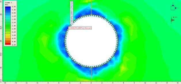
111 XIII MSFL MML Seismic loading h=0.3 Seismic loading v=-0.3 MAFL MSFL MML

112 XIV The locations of the MAFL, MSFL and MML change after applying seismic loads in each case of loading in the case of the vertical joint. B.3 Diagonal joint (45) B.3.1 Strong rock Static loading Seismic loading h=0.3& v=-0.2 MAFL MSFL MML

113 XV Seismic loading h=0.3 Seismic loading v=-0.3 MAFL MSFL MML The locations of the MAFL do not change. The MSFL and MML change under the different combinations of seismic loads in strong rocks in the case of the diagonal joint. The locations of the MAFL occur at the point of intersection between the horizontal and vertical planes of weakness and the tunnel lining in strong rocks but not in the case of the diagonal joints.

114 XVI B.3.2 Weak rock Static loading Seismic loading h=0.3& v=-0.2 MAFL MSFL MML Seismic loading h=0.3 Seismic loading v=-0.3 MAFL

115 XVII MSFL MML The locations of the MAFL, MSFL and MML change after applying seismic loads in each case of loading in the case of the diagonal joint B.4 Summary of the results 10 m diameter Static loading on strong rock Seismic loading h=0.3on strong rock Seismic loading v=-0.3 on strong rock Seismic loading h=0.3& v=-0.2 on strong rock MAFL(MN) MAFL(MN) MAFL(MN) MAFL(MN) without m diameter Static loading on strong rock Seismic loading h=0.3on strong rock Seismic loading v=-0.3 on strong rock Seismic loading h=0.3& v=-0.2 on strong rock MSFL(MN) MSFL(MN) MSFL(MN) MSFL(MN) without

116 XVIII 10 m diameter Static loading on strong rock Seismic loading h=0.3on strong rock Seismic loading v=-0.3 on strong rock Seismic loading h=0.3& v=-0.2 on strong rock MML(MN*m) MML(MN*m) MML(MN*m) MML(MN*m) without m diameter Static loading on weak rock Seismic loading h=0.3on weak rock Seismic loading v=-0.3 on weak rock Seismic loading h=0.3& v=-0.2 on weak rock MAFL(MN) MAFL(MN) MAFL(MN) MAFL(MN) without m diameter Static loading on weak rock Seismic loading h=0.3on weak rock Seismic loading v=-0.3 on weak rock Seismic loading h=0.3& v=-0.2 on weak rock MSFL(MN) MSFL(MN) MSFL(MN) MSFL(MN) without

117 XIX 10 m diameter Static loading on weak rock Seismic loading h=0.3on weak rock Seismic loading v=-0.3 on weak rock Seismic loading h=0.3& v=-0.2 on weak rock MML(MN*m) MML(MN*m) MML(MN*m) MML(MN*m) without

118 XX C. Case study 2 experiment (friction angle from 10 to 20 ) C.1 Strong rock Static loading Seismic loading h=0.3& v=-0.2 MAFL MSFL MML Seismic loading h=0.3 Seismic loading v=-0.3 MAFL

119 XXI MSFL MML C.2 Weak rock Static loading Seismic loading h=0.3& v=-0.2 MAFL MSFL

120 XXII MML Seismic loading h=0.3 Seismic loading v=-0.3 MAFL MSFL MML