Bridge Load Rating JOINT TRANSPORTATION RESEARCH PROGRAM. Rafael R. Armendariz. Mark D. Bowman

Transcription

1 JOINT TRANSPORTATION RESEARCH PROGRAM INDIANA DEPARTMENT OF TRANSPORTATION AND PURDUE UNIVERSITY Bridge Load Rating Rafael R. Armendariz Mark D. Bowman SPR-3816 Report Number: FHWA/IN/JTRP-2018/07 DOI: /

2 RECOMMENDED CITATION Armendariz, R. R., & Bowman, M. D. (2018). Bridge load rating (Joint Transportation Research Program Publication No. FHWA/IN/JTRP-2018/07). West Lafayette, IN: Purdue University. AUTHORS Rafael R. Armendariz Graduate Research Assistant Lyles School of Civil Engineering Purdue University Mark D. Bowman, PhD Professor of Civil Engineering Lyles School of Civil Engineering Purdue University (765) Corresponding Author ACKNOWLEDGMENTS Our research team is most grateful to the following Research Study Advisory Committee members, who provided outstanding support during this study: Tim Wells, Merril Dougherty, Sean Hankins, Jeremy Hunter, Jose Ortiz, and Mark Swiderski. Thanks are also extended to Mr. Xiao Zhang, who assisted with the evaluation and analysis of the multi-plate arch structure as part of his summer research experience, and to Mr. Stefan Leiva, who assisted with the installation of strain gages on the Doan s Creek Bridge. Special thanks are extended to Tim Wells, who worked tirelessly to assist the research team on site visits to various bridges and even helped with of the Doan s Creek field site measurements. We would also like to recognize the many personnel and staff in both the Crawfordsville District and Vincennes District who provided assistance with the Roaring Creek and Doan s Creek bridge load tests. Without their help the load tests could not have been conducted. JOINT TRANSPORTATION RESEARCH PROGRAM The Joint Transportation Research Program serves as a vehicle for INDOT collaboration with higher education institutions and industry in Indiana to facilitate innovation that results in continuous improvement in the planning, design, construction, operation, management and economic efficiency of the Indiana transportation infrastructure. Published reports of the Joint Transportation Research Program are available at NOTICE The contents of this report reflect the views of the authors, who are responsible for the facts and the accuracy of the data presented herein. The contents do not necessarily reflect the official views and policies of the Indiana Department of Transportation or the Federal Highway Administration. The report does not constitute a standard, specification or regulation. COPYRIGHT Copyright 2018 by Purdue University. All rights reserved. Print ISBN:

3 TECHNICAL REPORT STANDARD TITLE PAGE 1. Report No. 2. Government Accession No. 3. Recipient's Catalog No. FHWA/IN/JTRP-2018/07 4. Title and Subtitle Bridge Load Rating 7. Author(s) Rafael R. Armendariz, Mark D. Bowman 9. Performing Organization Name and Address Joint Transportation Research Program Hall for Discovery and Learning Research (DLR), Suite S. Martin Jischke Drive West Lafayette, IN Sponsoring Agency Name and Address Indiana Department of Transportation State Office Building 100 North Senate Avenue Indianapolis, IN Report Date April Performing Organization Code 8. Performing Organization Report No. FHWA/IN/JTRP-2018/ Work Unit No. 11. Contract or Grant No. SPR Type of Report and Period Covered Final Report 14. Sponsoring Agency Code 15. Supplementary Notes Prepared in cooperation with the Indiana Department of Transportation and Federal Highway Administration. 16. Abstract The inspection and evaluation of bridges in Indiana is critical to ensure their safety to better serve the citizens of the state. Part of this evaluation includes bridge load rating. Bridge load rating, which is a measure of the safe load capacity of the bridge, is a logical process that is typically conducted by utilizing critical information that is available on the bridge plans. For existing, poorly-documented bridges, however, the load rating process becomes challenging to adequately complete because of the missing bridge information. Currently, the Indiana Department of Transportation (INDOT) does not have a prescribed methodology for such bridges. In an effort to improve Indiana load rating practices INDOT commissioned this study to develop a general procedure for load rating bridges without plans. The general procedure was developed and it was concluded that it requires four critical parts. These parts are bridge characterization, bridge database, field survey and inspection, and bridge load rating. The proposed procedure was then evaluated on two bridges in Indiana that do not have plans as a proof of concept. As a result, it was concluded that load rating of bridges without plans can be successfully completed using the general procedure. A flowchart describing the general procedure was created to make the load rating process more user-friendly. Additional flowcharts that summarize the general procedure for different type of bridges were also provided. 17. Key Words load rating, bridges without plans, buried structures, load testing, finite element analysis 18. Distribution Statement No restrictions. This document is available to the public through the National Technical Information Service, Springfield, VA Security Classif. (of this report) 20. Security Classif. (of this page) 21. No. of Pages 22. Price Unclassified Form DOT F (8-69) Unclassified 86

4 Introduction EXECUTIVE SUMMARY BRIDGE LOAD RATING Bridge load rating is typically performed by utilizing critical information available on the bridge plans. This includes information about the span lengths, the sizes and dimensions of the bridge members, the type of materials used to construct the bridge, and other relevant information. This information is used to perform a structural analysis to determine the forces or stresses caused by Indiana legal loads. These forces or stresses are then compared with the strength limit states of the bridge to determine the corresponding load rating. Decisions on the need to post a particular bridge can then be made if the operating rating factor is determined to be less than unity. While the load rating process is logical and can be implemented for many of the bridges in Indiana, some bridges cannot be easily evaluated because they are poorly documented or do not have plans. Initial estimates provided by INDOT indicated that there are 53 bridges in the state inventory of bridges that fall into this category. If the bridges in the counties and cities were included, there would be hundreds of bridges that could not be readily load rated and evaluated. Currently, INDOT does not have a prescribed methodology to load rate and evaluate bridges without plans. Consequently, a standardized procedure is needed for such bridges. Hence, the primary objective of this study was to develop a general procedure for load rating bridges without plans. The evaluation of an open-spandrel reinforced concrete arch bridge was also examined as part of this study. This bridge, referred to as the Roaring Creek Bridge, was load-posted based on a simplified structural evaluation conducted for INDOT. This bridge is a main route for conventional traffic. Consequently, there was a need to examine the adequacy of the posting load to avoid costly detours. Findings A general procedure for load rating bridges without plans was developed. It was concluded that the procedure required four critical parts. These included bridge characterization, bridge database, field survey and inspection, and bridge load rating. The bridge characterization is used to create a list of variables required for the load rating calculations. These variables include but are not limited to material strength properties, geometric features, and strength and service limit states. The bridge database provides guidelines and recommendations for obtaining the unknown information discerned from the bridge characterization. It requires one to examine past and current historical inspection reports, conduct a survey of comparable bridge plans, and examine past standards used at the original time of construction. If the value of a parameter remains unclear, the most conservative value of that parameter is assumed based upon comparable historical information. The previous performance of the bridge should also be considered. The field survey supplements the unknown bridge information by collecting field measurements. A field inspection is also required to account for the condition of the structure during the load rating process. Drawings of the structure can be created by using the collected information. The drawings can then be used as the layout for the structural modeling to perform the bridge load rating. It was found that buried structures were among the most predominant type of bridges without plans in the Indiana state inventory of bridges. The research team identified particular bridge structures that would be utilized to evaluate the general procedure. The general procedure was evaluated on a flexible and rigid buried structure without plans. It was demonstrated that the general procedure can be utilized to successfully complete the bridge load rating of poorly documented structures. It was found that the controlling strength limit state for the flexible buried corrugated steel pipe bridge was the minimum of the wall area, buckling strength, and seam resistance. The controlling strength limit state for the rigid buried reinforced concrete arch bridge was the coupled action of axial compression load and flexure. The load rating of the latter bridge was performed using an iterative load rating method that required the use of an interaction diagram. The Roaring Creek Bridge was initially load-posted based upon a simplified structural analysis that showed that the controlling rating members were the floor beams. An experimental evaluation performed on one of the critical members of the bridge was performed and the results were compared with those obtained analytically. Both the experimental and analytical results showed that the bridge exhibited a higher load-carrying capacity than the initial restrictive load estimated for this bridge. Implementation The general procedure developed for use by INDOT can be applied to state-, county-, and city-owned bridges. As a result, INDOT now has a load rating methodology for the hundreds of bridges without plans in Indiana. A flowchart describing the general procedure was created to make the load rating process more user-friendly. Additional flowcharts that summarize the general procedure for different types of bridges were also provided. These flowcharts can then be used by the load rating engineer to ease the load rating process. The methodology adopted to perform the load rating of bridges without plans or other critical information could potentially lead to significant cost savings. If the load rating results in an operating rating factor greater than unity, there is no need to post the bridge. This allows a bridge rehabilitation or replacement to be scheduled in a more timely fashion if needed. Moreover, this could prevent possible detours that result in delays and inconvenience for the traveling public. Alternatively, it is also possible that the general procedure could lead to necessary bridge posting or closing; however, the end result would be improved safety for the public.

5 CONTENTS 1. INTRODUCTION Objective Scope LITERATUREREVIEW LoadRating Methods for Load Rating Bridges Without Plans GENERALPROCEDURE Bridge Characterization BridgeDatabase FieldSurveyandInspection BridgeLoadRating Proposed General Procedure FIELD ASSESSMENT First Field Assessment SecondFieldAssessment Selected Candidate Bridges CASESTUDYBRIDGENO Bridge Characterization FiledSurveyandInspection LoadRating CASESTUDYBRIDGENO Bridge Characterization BridgeDatabase FiledSurveyandInspection LoadRating REINFORCEDCONCRETEBOX Dimensions MaterialProperties Soil Parameters Reinforcement InstallationMethod ROARINGCREEKBRIDGE Overview LoadTesting RefinedAnalyses Experimental and Analytical Results LoadRating SUMMARYANDCONCLUSIONS REFERENCES APPENDICES Appendix A. AASHTO LRFD (2014) Live Load Distribution Through Earth Fills Appendix B. AASHTO SSHB (2002) Live Load Distribution Through Earth Fills Appendix C. Multi-Plate Arch Under Fill Load Rating Example Appendix D. Approximate Formulas for Compression- and Tension-Controlled Regions of an InteractionDiagram Appendix E. Doan s Creek Bridge Numerical Load Rating Input for Matlab Appendix F. Reinforced Concrete Box Bridges Evaluation AppendixG.Flowcharts... 79

6 LIST OF TABLES Table Page Table 2.1 Values for K b 3 Table 2.2 Condition Factor (CF) 5 Table 2.3 Inventory and Operating Ratings by NBI Condition Rating 5 Table 4.1 State Inventory of Bridges Without Plans in Indiana 9 Table 5.1 USCS Nomenclature 13 Table 5.2 Comparison between AASHTO System and the USCS 14 Table 5.3 Typical Values of Dry Unit Weight for Different Soils Classified by USCS 14 Table 5.4 Impact Factor for Structures with Soil Cover 15 Table 5.5 Load Factors and Load Modifiers for Flexible Buried Structures 15 Table 5.6 List of Variables for MPA-UF 17 Table 5.7 Cross-Section Properties of Steel Structural Plate 18 Table 5.8 Mechanical Properties for Design of Steel Structural Plate 18 Table 5.9 Minimum Longitudinal Seam Strengths 19 Table 5.10 Load Rating Results of Bridge No Table 6.1 Load Factors and Load Modifiers for Rigid Buried Structures 22 Table 6.2 List of Variables for RCA-UF 22 Table 6.3 Database of Survey of Comparable Plans 24 Table 6.4 Load Rating Results of Bridge No Table 7.1 List of Reinforced Concrete Box Dimensional Variables 32 Table 7.2 Modulus of Subgrade Reaction 33 Table 7.3 Modulus of Elasticity for Different Types of Soil 33 Table 7.4 Steel Reinforcement Variables 34

7 LIST OF FIGURES Figure Page Figure 3.1 Flowchart of general load rating procedure 8 Figure 4.1 Bridges visited during first field assessment 10 Figure 4.2 Bridges visited during second field assessment 11 Figure 5.1 Pipe-arch cross-section 16 Figure 5.2 Arranged bolt pattern in longitudinal seam 17 Figure 5.3 Measurement of depth of soil cover 17 Figure 5.4 Corrugated steel arch plan view, cross-section elevation, and corrugation size 18 Figure 6.1 Field inspection of the northeast arch 24 Figure 6.2 Doan s Creek Bridge: (a) plan view; (b) cross-section elevation 25 Figure 6.3 Section forces diagram for east span: (a) factored axial force; (b) factored bending moment; (c) factored shear force 26 Figure 6.4 Illustrative example of iterative process for computing the rating factor (RF) using an interaction diagram 27 Figure 6.5 Flowchart of iterative load rating process using an interaction diagram 28 Figure 6.6 Interaction diagram of arch member 29 Figure 6.7 Trucks configuration 30 Figure 6.8 Two trucks static loading 30 Figure 6.9 Strains recorded during load test: (a) crawl; (b) dynamic 31 Figure 7.1 Reinforced concrete box with soil cover dimensions 32 Figure 7.2 Top slab cross-section labeled for positive bending moment 34 Figure 8.1 Roaring Creek Bridge 35 Figure 8.2 Typical cross-section of the Roaring Creek Bridge 35 Figure 8.3 Strain gage layout 36 Figure 8.4 Trucks dimensions 36 Figure 8.5 Deck system model 37 Figure 8.6 Finite element model 38 Figure 8.7 Measured and predicted strains: (a) Test 1; (b) Test 2; (c) Test 3; and (d) Test 5 39 Figure 8.8 Estimated and predicted bending moment: (a) Test 1; (b) Test 2; (c) Test 3; (d) Test 5 40 Figure 8.9 Estimated and predicted shear force: (a) Test 1; (b) Test 2; (c) Test 3; (d) Test 5 41 Figure 8.10 Normalized maximum force effects: (a) bending moment; (b) shear force at critical section 41 Figure A.1 Longitudinal and transverse view of HL-93 design truck, one lane loaded 44 Figure A.2 Longitudinal and transverse view of HL-93 design tandem, one lane loaded 45 Figure A.3 Longitudinal and transverse view of HL-93 design truck, two lanes loaded 45 Figure A.4 Longitudinal and transverse view of HL-93 design tandem, two lanes loaded 45 Figure A.5 HL-93 design truck live load distribution through earth fills envelope 46 Figure A.6 HL-93 design tandem live load distribution through earth fills envelope 46 Figure B.1 Longitudinal and transverse view of HS-20 truck, one lane loaded 47 Figure B.2 Longitudinal and transverse view of HS-20 truck, two lanes loaded 48 Figure B.3 HS-20 truck live load distribution through earth fills envelope 48 Figure F.1 Concrete box three-dimensional view indicating two-dimensional strip 72 Figure F.2 Moment critical sections for reinforced concrete box without haunches (left) and with haunches (right) 73

8 Figure F.3 Shear critical sections for reinforced concrete box without haunches (left) and with haunches (right) 73 Figure F.4 Two-dimensional frame model showing location of nodes of critical sections for reinforced concrete box without haunches (left) and with haunches (right) 74 Figure F.5 Boundary conditions assuming two-dimensional frame model 74 Figure F.6 Two-dimensional frame model with soil springs 76 Figure F.7 Typical layout of soil-structure interaction model 76 Figure G.1 Flowchart for load rating multi-plate arch bridges with soil cover 79 Figure G.2 Flowchart for load rating reinforced concrete arch bridges with soil cover 80 Figure G.3 Flowchart for load rating reinforced concrete box bridges with soil cover 80 Figure G.4 Flowchart for load rating reinforced concrete slab bridges with soil cover 81

9 1. INTRODUCTION The process by which the structural condition of a bridge is determined is named bridge load rating. This process typically uses bridge information that can be found in plans or support design calculations so that a structural analysis and evaluation can be conducted. However, for bridges without plans the load rating can become challenging. Load testing is the most reliable technique and the one that provides the most accurate results when determining the load-carrying capacity of bridges with unknown details (Cuaron, Jauregui, & Wheldon, 2017). However, research conducted to evaluate bridges without plans is limited. Moreover, a prescribed rating value is usually assigned to bridges that do not have plans in lieu of more refined methods of evaluation, e.g., liveload testing. 1.1 Objective Currently, Indiana does not have a prescribed methodology to evaluate bridges without plans. Thus, the objective of this research project was to develop a general procedure to load rate bridges without plans. The procedure was developed in accordance with the AASHTO s (2011) Manual for Bridge Evaluation (MBE) and the Indiana Department of Transportation (INDOT, 2013, 2014, 2017) requirements. 1.2 Scope The procedure included the following steps: (a) bridge characterization, (b) bridge database, (c) field survey and inspection, and (d) load rating evaluation. This project delivered a standardized general methodology to address the rating evaluation of bridges that do not have plans or support design calculations. At the request of INDOT, special interest was devoted to bridges under soil cover. Two bridge candidates were selected from a list provided by INDOT of bridges without plans. The recommended general procedure was applied to the bridge test subjects to demonstrate its application. 2. LITERATURE REVIEW This section includes a description of the load rating process and methods available in the literature for load rating bridges without plans. 2.1 Load Rating Bridge load rating provides a basis for determining the safe load capacity of a bridge. Its primary focus is the assessment of the safety of bridges for live loads and fatigue. It requires engineering judgement in determining a rating value that is applicable to maintain the safe use of the bridge and arriving at posting and permit decisions (AASHTO, 2011). The MBE (AASHTO, 2011) sets forth criteria for the load rating and posting of existing bridges. These criteria are intended for use in evaluating the types of highway bridges commonly used in the United States that are primarily subjected to permanent loads and vehicular loads. Methods for evaluating extreme events such as earthquake, wind, ice, or fire are not included in the MBE (AASHTO, 2011). Rating of long-span bridges, and other complex bridges may involve additional considerations and loadings not specifically addressed in the MBE (AASHTO, 2011). The load rating methods, as per the MBE (AASHTO, 2011), are the Load and Resistance Factor Rating (LRFR), Load Factor Rating (LFR), and Allowable Stress Rating (ASR). The LRFR method was developed to provide uniform reliability in bridge load rating, load posting, and permit decisions. The LFR method provide safety criteria for bridge load rating based on load factors to reflect the uncertainty inherent in the load calculations. The ASR method combines the actual loadings to produce a maximum stress in the member, which is not to exceed the allowable or working stress. No preference is placed on any rating method by the MBE (AASHTO, 2011). However, it is common practice to use the rating method in accordance with the original adopted design philosophy. For example, a bridge designed by the Load Factor Design (LFD) philosophy would typically be rated using the LFR method. Yet, the same bridge could be rated by the LRFR and ASR methods. The LRFR and LFR methods are discussed in more detail in the following subsection as they are the preferred methodologies by INDOT (2017) Load and Resistance Factor Rating The LRFR method provides a rating consistent with the Load and Resistance Factor Design (LRFD) philosophy. The methodology uses load and resistance factors that have been calibrated based on structural reliability theory to achieve minimum target reliability for the strength limit state (AASHTO, 2011). In addition, the MBE (AASHTO, 2011) provides guidance on service limit states that are applicable to bridge load rating. Bridge evaluations are performed under different live load models. The evaluation live load models are comprised of the design live load, legal loads, and permit loads and represent a systematic approach to bridge load rating. Each live load model is evaluated by its own load rating procedure: (1) design load rating, (2) legal load rating, and (3) permit load rating. The results of each procedure serve specific evaluation criterion and guide the need for further evaluation to verify bridge safety or serviceability (AASHTO, 2011). The design load rating measures the performance of existing bridges based on the HL-93 loading and current LRFD design standards. It is a first-level assessment and consists of a design level reliability (Inventory) and a second lower-level reliability (Operating). Joint Transportation Research Program Technical Report FHWA/IN/JTRP-2018/07 1

10 Under the design load rating, bridges are screened for the strength limit state and the rating also considers all applicable serviceability limit states. The design load rating serves as a screening process to identify bridges that should be load rated for legal loads. Bridges that pass the design load rating at the Inventory level will have adequate capacity for all legal loads that fall within the LRFD exclusion limits. Bridges that pass the design load rating at the Operating level will have adequate capacity for AASHTO legal loads but not necessarily to all State legal loads, as some of these loads might be heavier than the AASHTO legal loads. The legal load rating provides a single safe load capacity (for a given truck configuration) applicable to AASHTO and State legal loads. Strength is the primary limit state under the legal load rating; service limit states are selectively applied (AASHTO, 2011). Live load factors are selected based upon traffic conditions at the site. The results of the legal load rating establishes the need for load posting or strengthening of the bridge. A bridge that passes the legal load rating does not need any further action and can be rated under the permit load rating. Alternatively, actions such as load posting, replacement or repair activities, or closing of the bridge are taken when the bridge fails to pass the legal load rating. The MBE (AASHTO, 2011) allows the use of higher levels of evaluation when a bridge fails to pass the legal load rating. A refined structural analysis, load testing, the use of site-specific load factors, or direct safety assessment are among the higher level evaluation methods. Bridges that rate satisfactory under the legal load rating using higher level of evaluation methods can be rated under the permit load rating. Alternatively, load posting or strengthening of the bridge is needed when higher level of evaluation methods demonstrate that bridge safety and serviceability are unsatisfactory. The permit load rating checks the safety and serviceability of bridges for oversized trucks. This third-level assessment should only be applied to bridges that have adequate capacity to carry legal loads. Calibrated load factors by permit type and traffic conditions at the site are specified under the MBE (AASHTO, 2011). The load rating is generally expressed as a rating factor for a particular live load model. The following general expression (Equation 2.1) is used to determine the load rating of each component and connection subjected to a single force effect, i.e., axial, flexure, or shear. RF~ C{(c DC)(DC){(c DW )(DW)+(c P )(P) (c LL )(LLzIM) ð2:1þ where, C is the capacity of the member; DC is the dead load effect on the member; DW is the wearing surface load effect on the member; P is the permanent loads other than dead loads; LL is the live load effect on the member; IM is the dynamic load allowance due to live loading; c DC is the LRFD load factor for dead load; c DW is the LRFD load factor for wearing surface load; c P is the LRFD load factor for permeant loads other than dead loads; and c LL is the evaluation live load factor. The capacity, C, should be as specified in the AASHTO LRFD Bridge Design Specifications (AASHTO, 2014). Strength is the primary limit state; service and fatigue limit states are selectively applied. The nominal strength of the component needs to reflect its current condition Load Factor Rating The LFR method is based on analyzing a bridge subjected to multiples of the actual loads (AASHTO, 2011). Load factors are used to reflect the uncertainty of the load calculations. The rating is obtained so that the effects of the factored load does not exceed the strength of the member. The LFR is broken down into two levels, each with a different evaluation level of safety: Inventory and Operating levels. The Inventory level usually corresponds to the customary design level of stress but reflects the existing bridge and material conditions (AASHTO, 2011). The Operating level generally describes the maximum permissible live load to which the bridge may be subjected (AASHTO, 2011). The following general expression (Equation 2.2) is used to determine the load rating of the bridge: RF~ C{A 1D A 2 L(1zI) ð2:2þ where, C is the capacity of the member; D is the dead load effect on the member; L is the live load effect on the member; I is the impact factor; and A 1 and A 2 are the factors for dead load and live load, respectively. The load factor for live load A 2 depends on the rating level to account for the different levels of safety. The live load effect to be used in the general load rating equation should be determined using the HS-20 truck and lane loading as specified in the MBE (AASHTO, 2011). The capacity of the member should be as specified in the load factor sections of the AASHTO s (2002) Standard Specifications for Highway Bridges (AASHTO SSHB). The nominal strength calculations need to take into account deterioration or section loss of the member Load Rating Through Load Testing The MBE (AASHTO, 2011) provides recommendations to load rate bridges that lack existing as-built information by the use of load testing. Two types of load tests can be performed to evaluate a bridge response: diagnostic test or proof test. In addition to the MBE (AASHTO, 2011), the National Cooperative Highway Research Program (NCHRP, 1998) provide guidelines for both types of load test. A diagnostic test uses a predetermined load, which is near the bridge s load-carrying capacity, placed at 2 Joint Transportation Research Program Technical Report FHWA/IN/JTRP-2018/07

11 several locations along the bridge to observe and measure its response. The measured response and its load effects in one or more critical bridge members are compared with that obtained from theory (analytical model). The diagnostic test serves to verify and adjust the predictions of an analytical model. The calibrated analytical model is then used to compute the load-rating factors (AASHTO, 2011). Therefore, bridges in which their strength is underestimated by an analytical model, e.g., higher load distribution mechanisms, redundant spans, etc., are suitable candidates for diagnostic load testing. In a proof test, the bridge is subjected to specific loads and its response is monitored to determine whether the bridge can carry these loads without damage. The loads are placed in increments to detect early signs of distress or nonlinear behavior (AASHTO, 2011). The proof test is terminated when a predetermined load is reached or a limit state is exceeded. According to the MBE (AASHTO, 2011) bridges that are suitable candidates for proof load testing may be separated into two groups: known and hidden bridges. Known bridges are those whose make-up is known and can be load rated analytically. For these bridges a proof test is called for when calculated load ratings are low and the load testing may provide realistic results and higher ratings (AASHTO, 2011). Hidden bridges are those for which a load rating cannot be conducted due to insufficient information on their internal details and configuration (AASHTO, 2011). Thus, bridges without construction plans, design plans or both fall into this category, for which, a proof test is needed to determine a realistic live-load capacity. In a survey (Cuaron et al., 2017) submitted to the fifty state Departments of Transportation (DOTs) information was requested regarding their load rating procedures for bridges without plans. About 52% of those who responded indicated that they conduct load tests; diagnostic test being the most common. The procedure set forth for load rating bridges through load testing is found in the MBE 8.8 (AASHTO, 2011). The procedure when using diagnostic test consists in calculating an adjustment factor K (Equation 2.3), which is multiplied times the rating factor obtained from a simplified load rating analysis. RF T ~RF C K ð2:3þ where, RF T is the load rating factor updated from the live-load test data; and RF C is the calculated rating factor obtained from a simplified rating analysis. The adjustment factor K is calculated by computing the K a and K b factors (Equation 2.4). The factor K a accounts for the benefit of the load test, if any, and the consideration of the section properties, i.e., the section modulus resisting the applied load test. The factor K b is related to the understanding of the load test results when compared with those predicted by theory (AASHTO, 2011). K~1zK a K b ð2:4þ If the value of K is greater than unity, then the response of the bridge observed during the live-load test is more favorable than that computed from the simplified load rating analysis. Alternatively, if the value of K is less than unity, then the response of the bridge observed during the live-load test is worse than that calculated using simplified load rating techniques. The procedure outlined in the MBE (AASHTO, 2011) consists in computing the factor K a through the following expression (Equation 2.5): K a ~ e C e T {1 ð2:5þ where, e T is the maximum strain of the member measured during the live-load test; and e C is the corresponding strain predicted using the analytical model at the position where e T was measured. The K b factor requires the user to identify if the member behavior can be extrapolated to 1.33W, where W is the unfactored gross load effect. To check this criterion, the analytical model is loaded with the load increased by 33% and then checked to determine if the members of the bridge remain in the linear elastic range. Table 2.1 shows the values of K b. 2.2 Methods for Load Rating Bridges Without Plans The procedures named Steel Area Method (SAM) and Simplified Method (SM) were developed to load TABLE 2.1 Values for K b (adapted from AASHTO, 2011) Can member behavior be extrapolated to 1.33W? Magnitude of Test Load Yes No T W v0:4 0:4v T W v0:7 T W w0:7 K b!! 0!! 0.8!! 1!! 0!! 0!! 0.5 Note: T 5 unfactored test vehicle effect; W 5 unfactored gross rating load effect. Joint Transportation Research Program Technical Report FHWA/IN/JTRP-2018/07 3

12 rate reinforced concrete bridges without plans (Huang & Shenton, 2010). The SAM procedure uses theoretical analysis and live-load test measurements to estimate the area of reinforcing steel. The SM procedure utilizes measured live load strains to directly estimate the bridge load rating. The load rating using the SM is based on the ASR method and is calculated using the following expression (Equation 2.6): RF~ e all{e DL e LL (1zI) ð2:6þ where, e all is the allowable strain; e DL is the dead load strain; e LL is the live load strain; and I is the impact factor. For concrete structures designed by ASD philosophy the maximum service strain at the inventory level is based on a working stress lower than the yielding of the rebar stress. Thus, e all can be estimated with reasonable confidence by Equation 2.7 by knowing the age of the bridge and with knowledge of the grade of reinforcing steel common for that era (Huang & Shenton, 2010). e all ~ 0:55f y E s ð2:7þ The dead load strain can be estimated by the simple relationship presented in the expression below (Equation 2.8): e DL ~ M DL e LL ð2:8þ M LL where, M DL and M LL are the theoretical moments due to dead load and live load produced by the test truck, respectively; and e LL is the measured strain under the test truck. The SAM was extended to accommodate more realistic general load configurations used in a typical load test. The expressions (Equation 2.9 and Equation 2.10) developed in the SAM involve the use of strain or displacement measurements and are referred to as the moment-strain stiffness and moment-displacement stiffness, respectively. bx 2 d{ x3 M 3 e cb ~E c ~k strain ð2:9þ 2(h{x) M correct D 8 ~ f r I! g 3 2 < y t I g z 1{ f r I g 4 y t : M a 1 z bx2 (d{x) 3 bx3 g~k deft 2 M a! ð2:10þ The SAM consists in collecting strain or displacement measurements on the critical components of a concrete bridge. Using the known axle weight and spacing of the test truck, the moments at the location where the measurements were recorded are computed analytically. The analytical moments are then plotted against the measurements obtained from the live-load test and a linear regression is fitted to calculate the slope, which value corresponds to either k strain or k defl depending whether strain or displacement measurements were recorded. Using the expressions above the neutral axis position of the cross-section x is solved to estimate the area of reinforcing steel using the following expression (Equation 2.11): A s ~ bx2 2n(d{x) ð2:11þ The expressions described above were tested on a reinforced concrete slab bridge to estimate the reinforcing steel. Both strain and displacement were measured along the bridge during a live-load test. The sample bridge was in good condition with no skew and had low traffic volume. Plans of the tested bridge were available so comparisons between the estimated and actual reinforcing steel could be made. The study concluded that the developed expressions were satisfactory in estimating the reinforcing steel of the tested concrete slab bridge. However, displacement measurements were more reliable than concrete strain measurements, cracking moment measured in the liveload test was lower than the one estimated based on theory, and the procedure was sensitive to load distribution factors (DFs). Therefore, it was recommended to obtain DFs from field load testing when possible. The use of Windsor Probe testing combined with a Ferroscan nondestructive testing system for the load rating of reinforced concrete slab bridges without plans was investigated by Cuaron et al. (2017). The concrete strength was estimated using the Windsor Probe and the rebar size, spacing, cover, and length were estimated using a Ferroscan system. The authors reported that the Ferroscan system was not very effective in determining the rebar size where the concrete cover was three inches or more, usually top reinforcing steel for concrete slab bridges (Cuaron et al., 2017). Instead, the reinforcement was estimated based upon historical ratio of top to bottom area of reinforcing steel per linear foot. A total of twenty-three bridges were evaluated, however, the Windsor Probe testing failed, i.e., required number of probes did not embed, at twelve of them. A nominal concrete strength of 3,000 psi were used for those cases. As-built plans were created based on field measurements and estimated rebar layout. The plans were used to model each bridge to determine the load ratings. The ratings were performed using the nominal concrete compressive strength of 3,000 psi and the measured concrete strength obtained from the Windsor Probe when available. Overall, the results showed that on average there was an increase of 16% on the load ratings when using the measured concrete compressive strength obtained from the Windsor Probe testing. In addition, the authors claimed that that the use of basic nondestructive testing 4 Joint Transportation Research Program Technical Report FHWA/IN/JTRP-2018/07

13 along with the implementation of simple structural analysis techniques proved to be an effective method for estimating the load-carrying capacity of reinforced concrete slab bridges without plans (Cuaron et al., 2017). Several DOTs have their own policy for load rating bridges without plans, however, their ratings are usually based on the National Bridge Inventory (NBI) condition rating. For example, the Texas DOT Policy assigns an HS-15 inventory rating and HS-20 operating rating for reinforced concrete structures with unknown details and no sign of structural distress. If the structure is over 4 years old and the NBI condition rating is less than 5 for Item 58 (Deck) and less than 6 for Item 59, 60, or 62 (Superstructure, Substructure, or Culvert) the bridge is load posted at the inventory level (TxDOT, 2013). This procedure may be followed given that the following conditions are met: 1. The bridge has been carrying unrestricted traffic. 2. There are no signs of significant distress on the bridge. 3. The bridge exhibits proper span-to-depth ratio. 4. The construction details should match the specifications current at the time of estimated construction date. 5. The appearance of the bridge shows that construction was done by a competent builder. Additionally, if the bridge was built prior 1950, then the amount of reinforcing steel can be estimated based on a percentage of the gross area of the main beams (if tee-beam construction), or depth of slab (if slab construction). Oregon DOT policy specifies that if the bridge has a history of successfully carrying Oregon legal loads and the NBI condition rating is greater than or equal to fair, the maximum moment effect from the legal load is assumed to result in a rating factor equal to unity (ODOT, 2013), i.e., the capacity is assumed to be equal to the legal load that produced the largest load effect. The inventory rating factor is considered proportional to the legal load effects (Equation 2.12). The inventory rating factor (Equation 2.12) is modified to accommodate the live load factor that corresponds to the operating level when using the LFR method (Equation 2.13). RF HS20{Inventory ~ M Legal (CF) ð2:12þ M HS20 RF HS20{Operating ~(RF HS20{Inventory ) 5 3 ð2:13þ where, M Legal is the maximum moment load effect of Oregon legal loads; M HS20 is the maximum moment load effect of the HS-20 truck or design lane load; and CF is the condition factor based on the NBI condition rating as shown in Table 2.2. An exhaustive search for plans and shop drawings for bridges with unknown details is conducted and documented as per Idaho Transportation Department (ITD) (2016). If details cannot be found then the load rating is performed for a HS-20 truck based on the lowest NBI condition rating as shown in Table 2.3. TABLE 2.2 Condition Factor (CF) (adapted from ODOT, 2013) NBI Item 59 (Superstructure) Condition Rating Condition Factor (CF) 5 Fair Condition or better Poor Condition Serious Condition Critical Condition 0.12 TABLE 2.3 Inventory and Operating Ratings by NBI Condition Rating (adapted from ITD, 2013) Rating Factor Rating in Tons b Lowest NBI Condition Rating a Inventory Operating Inventory Operating c c c or0 c a Lowest NBI item for either 59 (superstructure), 60 (substructure), or 62 (culvert). b Based on HS 20 truck with a weight of 36 tons. c Indicate that weight limit posting for state legal loads may be considered. Joint Transportation Research Program Technical Report FHWA/IN/JTRP-2018/07 5

14 3. GENERAL PROCEDURE The common practice for load rating bridges without plans, based on the literature search conducted for this project, are load testing or assigned prescribed rating values based upon the NBI condition rating or the use of simplified load rating analysis and engineering judgement. Two procedures, developed particularly for concrete bridges, were also examined and, in general, involved estimating the reinforcing steel by either load testing and theoretical analysis or direct estimation using a Ferroscan system. It was evidenced that a prescribed methodology applicable to all bridges without plans that can be followed systematically is not currently available in the literature. Moreover, INDOT does not have such methodology and, therefore, a general procedure for load rating bridges without plans was developed. The general procedure consisted of: (a) bridge characterization, (b) bridge database, (c) field survey and inspection, and (d) bridge load rating. Each step is described in the following subsections. 3.1 Bridge Characterization Bridge characterization is defined herein as identifying bridge information required for a rating evaluation. Most bridges share common information such as span (simple, continuous, cantilever), material (stone, timber, concrete, steel), and form (beam, arch, truss, etc.). However, the challenge is that bridge information tends to be specific to a particular bridge type. For example, a reinforced concrete slab bridge has different information to a steel truss bridge. For concrete bridges the characterization may include specified concrete compressive strength, reinforcing steel yield strength, rebar size and layout. For steel bridges the characterization may include structural steel grade, plate thickness, and bolt type. In addition to section and material properties, the bridge characterization includes the identification of the additional components needed when checking the bridge limit states. 3.2 Bridge Database Historical bridge inspection reports should be collected as they contain invaluable bridge information. Features such as year of construction, type of bridge, average daily truck traffic (ADTT), geometric data, among other information can be found in these reports. It is recommended to conduct a comparison of current and past inspection reports so that the evolution of the condition of the structure can be assessed. Such comparison can potentially reveal signs of deterioration the structure has experienced or if it has been carrying unrestrictive traffic. Additional information such as repair or replacement activities conducted on the structure need to be identified if present, e.g., bridge widening or overlay. It is possible that rehabilitation plans are available so that missing bridge information can be supplemented. A survey of comparable plans should be conducted using the year of construction and bridge type. Material properties used at the time of original construction or design considerations pertaining to that era can potentially be discerned by collecting bridge information from comparable plans. ASTM and AASHO/AASHTO specifications typically used at the time of original construction should be collected and examined to complement the bridge database. In addition, MBE 6A.5.2, 6A.6.2, 6B.5.2, and 6B.5.3 (AASHTO, 2011) can be used to estimate unknown material properties in lieu of comparable plansorpaststandards. 3.3 Field Survey and Inspection A field survey and inspection should be performed to complement the missing bridge information. Surveying should be conducted so geometrical features of the bridge can be identified and measured. A thorough inspection of the structure should be conducted to identify any signs of significant distress, deterioration, or deformation. The findings on the condition of the bridge outlined in the inspection reports should be corroborated with the field inspection. The condition of the structure can then be accounted in the rating process. Lastly, sketches of the bridge are created from the bridge information collected from the database and field measurements. 3.4 Bridge Load Rating Traditional load rating techniques are usually suitable for bridges with no signs of significant distress or deformation and where all or most of the missing information was collected. For bridges where the information is incomplete, conventional load rating techniques can be used to estimate an initial bridge rating. For example, the rating engineer could conservatively assume the minimum reinforcement detail pertaining the era of original construction to estimate a rating for reinforced concrete bridges where the reinforcing steel detail remains unknown. When traditional rating practices result in unsatisfactory load ratings, more refined analysis should be investigated. A refined structural analysis, e.g., finite element method (FEM), is one alternative of a higher method of evaluation. Alternatively, if the information to characterize the bridge was insufficient, or sign of significant distress is encountered on a structure, or thereisreasontobelievethat the bridge response is not being properly captured by a structural model, then live-load testing can be conducted. Research has shown that nondestructive testing is a powerful tool for bridge load rating. For example, liveload testing, in-service monitoring and the use of sitespecific data were investigated in the Darley Road Bridge, Delaware, to improve its rating (Bhattacharya, Li, & Chajes, 2005; Chajes, Shenton, & O Shea, 2000). Also in Delaware, an unintended composite action of a 6 Joint Transportation Research Program Technical Report FHWA/IN/JTRP-2018/07

15 posted, steel-girder-and-slab bridge was revealed through nondestructive evaluation methods. This study showed that the posting levels on the bridge were unnecessary (Chajes, Mertz, & Commander, 1997). Additional benefits of live-load testing consist of using test data to update an analytical model to potentially provide a higher rating evaluation while maintaining conservatism (Sanayei, Phelps, Sipple, Bell, & Brenner, 2012) or adjust bridge ratings obtained from simplified structural analysis to account for in-situ bridge behavior (Sanayei, Reiff, Brenner, & Imbaro, 2015). 3.5 Proposed General Procedure A general procedure was developed to provide a standard method to follow when conducting a load rating for a bridge that has no plans or very poor documentation. The recommended general procedure is as follows (Figure 3.1): A. Bridge characterization 1. Identify the bridge that needs to be load rated. 2. Distinguish bridge span (simple, continuous, cantilever), materials (steel, concrete, masonry), and form (beam, arch, truss, girder, etc.). 3. Conduct a literature search of the type of bridge in consideration, e.g., simple span reinforced concrete slab bridge, continuous span steel girder bridge, twospan masonry arch bridge, etc. i. Summarize the information that would be required to conduct a structural and rating evaluation. ii. Summarize the additional features required when checking the bridge limit states during the load rating process. 4. Create a list of the bridge information discerned from the previous steps. B. Bridge database 1. Locate and examine current and past bridge inspection reports. i. Identify geometric data, i.e., span lengths, presence of skew, roadway width, member dimensions, etc. ii. Assess bridge condition, i.e., review comments on signs of distress or deterioration and if bridge has been carrying unrestrictive traffic. iii. Identify repair and replacement activities, e.g., bridge widening or overlay, and locate rehabilitation plans if available. 2. Conduct a survey of comparable plans based upon the bridge type identified in previous steps and year range pertaining original time of construction. i. Identify specifications on material properties. ii. Identify characteristic geometrical data. iii. Identify characteristic design features and considerations. 3. Examine ASTM and AASHO/AASHTO specifications pertaining the era of original time of construction. i. Review information regarding material properties, design considerations, and design philosophy. 4. Create a database using the information collected from comparable plans, historical inspection reports and standards. C. Field survey and inspection 1. Measure bridge geometric features. 2. Conduct a thorough inspection. Check and record signs of deterioration, deformation, or distress. 3. Corroborate bridge condition specified in the inspection reports. 4. Create bridge drawings based on database and field measurements. D. Bridge Load rating 1. Use of traditional rating techniques. i. If most or all the bridge information is collected. ii. If the bridge shows no signs of significant distress, deterioration, or excessive deformation. iii. For bridges when information is incomplete, traditional rating techniques can be used to conservatively estimate an initial bridge rating. For example, use minimum reinforcement ratio utilized in design at the original time of construction for reinforced concrete bridges where reinforcement details remain unknown. 2. Use of refined structural analysis. i. If traditional rating techniques result in unsatisfactory rating levels. ii. Use of finite element method (FEM) models that could effectively capture the bridge response. For example, unintended composite action or higher mechanisms of load distribution. From such analyses, higher ratings could potentially be attained. 3. Use of load testing. i. If most of the information to characterize the bridge remains unknown. ii. If significant signs of deterioration or distress is present. iii. There is reason to believe that the bridge response if not being properly captured by a structural model. iv. Test data used to update an analytical model so that ratings at higher levels of load can be estimated. v. Test results used to adjust bridge ratings obtained from simplified bridge modeling to account for in-situ bridge behavior as per the MBE (AASHTO, 2011) and NCHRP (1998). Joint Transportation Research Program Technical Report FHWA/IN/JTRP-2018/07 7

16 Figure 3.1 Flowchart of general load rating procedure. 8 Joint Transportation Research Program Technical Report FHWA/IN/JTRP-2018/07

17 4. FIELD ASSESSMENT A list of state-owned bridges without plans was provided by INDOT (Table 4.1). The list consisted of fifty-three bridges, where twenty-nine of them were bridges with soil cover. Thus, at the request of INDOT, a special interest was devoted to bridges with under fill since these type of bridges constituted about half of the bridges without plans identified in the INDOT list. Two field trips were scheduled to visit some of the bridges included in the INDOT list. The first field trip was conducted on June It originally included the visit of five multi-plate arch under fill (MPA-UF) and three reinforced concrete arch (RCA) bridges. The second field visit was carried through following the next month. It included the visit of four reinforced concrete arch under fill (RCA-UF), one MPA-UF, and one reinforced concrete box under fill (RCB-UF) bridges. The field trips evidenced those bridges that were more suitable to use as candidates to apply the proposed general procedure. Type of bridges with higher sampling number and close to the West Lafayette campus were the preferred option. In addition, observations were made regarding those bridges that were more suitable for load testing, if required. 4.1 First Field Assessment The following bridges, identified herein by their bridge number, were visited during the first field assessment (Figure 4.1). A brief description of each bridge is presented as follows. I ADJ. This bridge has four oval-shaped pipes. The bridge is under a frontage road, therefore, no heavy live loads were observed during the field visit. The diameter of the pipes is not large enough to provide adequate access for sensor installation. Overall, this bridge was not considered as a suitable candidate if bridge instrumentation weretoberequired. TABLE 4.1 State Inventory of Bridges Without Plans in Indiana Type of Bridge Description Abbreviation Qty. Multi-Plate Arch Under Fill MPA-UF 14 Reinforced Concrete Arch RCA 11 Reinforced Concrete Arch Under Fill RCA-UF 5 Reinforced Concrete Box Under Fill RCB-UF 5 Precast Concrete Slab Under Fill PCS-UF 2 Precast Concrete Arch Under Fill PCA-UF 2 Steel Thru Truss STT 2 Riveted Plate Girder RPG 2 Prestressed Concrete Box Beam PCBB 1 Steel Box Girder SBG 1 Continuous Steel Girder SCSG 1 Prestressed Concrete I-Beam PCIB 1 Reinforced Concrete Slab RCS 1 Precast Concrete Beam PCB 1 Welded Girder Rigid Frame WRGF 1 Reinforced Concrete Slab Under Fill RCS-UF 1 Bailey Truss BT 1 Metal Pipe Arch MPA 1 I This bridge is categorized as a MPA- UF. It has four oval-shaped pipes where the structural length is at least greater or equal to the soil cover (based upon the observations made at that time). This bridge is not a good candidate to instrument due to difficulties in accessibility to the site This structure, located in Miami County, has three circular-shaped pipes. It was observed that the pipes were small in diameter, thus, hindering the instrumentation of the bridge, if needed. In addition, accessibility and availability of electricity may present an issue when monitoring This MPA-UF structure, also located in Miami County, has three circular pipes with fairly good accessibility. However, the diameter of the pipes may not be suitable for instrumentation due to their size, which might difficult its access The last MPA-UF structure that was observed is located on US 24. The type of road where the bridge is located indicated that heavy live load traffic was present (some semi-trailer trucks were observed). The bridge was comprised of three circular pipes with diameters large enough, feature which eases the instrumentation of the bridge, if needed. Accessibility to the bridge was not very good since it was delimited by a wire fence. Electricity access points were not readily evident. Although this might arise as an issue for long-term monitoring, it would not be a concern for short-term monitoring as a portable generator could be used as a power source. Overall, this bridge was considered a suitable candidate for instrumentation, mainly because of its larger diameter size A. The bridge is located on US 35 in Cass County and is categorized as a RCA. This was a one-span bridge with two lanes. From the observations made during the field assessment, the bridge, as well as the deck, looked in good shape. It was observed that the bridge had been widened on both sides. It was believed that precast concrete box beams were used for the widening of this bridge based upon the observations made. It was discerned from the field assessment that accessibility at the bottom of the bridge was fairly good for instrumentation. However, closing one lane if load testing were to be performed might produce traffic congestion since the bridge has only two lanes This four-span arch bridge crosses the Eel River and is located in Logansport, IN. Upon the arrival to the site, it was noted that the bridge was under repair. The spandrel walls were removed and the debris were laid on the side of the bridge. The steel reinforcement was exposed on the debris of the spandrel walls. Although the bridge was originally classified as RCA, upon the inspection it was observed that the structure was an earthen-filled arch bridge, since the soil fill was exposed upon the removal of the spandrel walls. It was also noted that one of the piers was heavily deteriorated. Upon conversations held with personnel of the construction firm responsible for the maintenance activities, it was communicated that the repair activities started June 2 and expected to finish by Joint Transportation Research Program Technical Report FHWA/IN/JTRP-2018/07 9

18 Figure 4.1 Bridges visited during first field assessment. 10 Joint Transportation Research Program Technical Report FHWA/IN/JTRP-2018/07

19 Thanksgiving of Based on the observations made during the field assessment, it was concluded that this bridge could be a suitable candidate for instrumentation and monitoring since one of the spans was immediately located above ground, making it relatively convenient for sensor installation This RCA structure crosses the Harvey Creek and is located on SR 25. It is a one-span arch bridge and accessibility underneath the bridge was inconvenient, deeming this bridge not suitable for instrumentation. 4.2 Second Field Assessment The following bridges, identified herein by their bridge number, were visited during the second field assessment (Figure 4.2). A brief description of each bridge is presented as follows A. This RCA-UF bridge is located in Vigo County. It was noticed during the field assessment that this bridge carries a railroad line. It seemed that the railroad line was still active. This bridge was immediately discarded as a suitable candidate since it is a railroad bridge instead of a traffic bridge This two-span RCA-UF bridge is also located in Vigo County and caries SR 46. Access to underneath the bridge was inconvenient due to the dense vegetation surrounding the area. Although appropriate accessibility is ideal when instrumenting a bridge, this was not the case here. However, this could be solved by clearing some of the vegetation found near the bridge. Figure 4.2 Bridges visited during second field assessment. Joint Transportation Research Program Technical Report FHWA/IN/JTRP-2018/07 11

20 In addition, the elevation between the arch bottom surface and ground level was estimated to be less than 7 ft., which potentially made it a suitable candidate for sensor installation because of its readily reach to the bottom surface of the structure This structure crosses a branch of the Doan s Creek and it is a two-span RCA-UF. The bridge looked in good shape based on the observations made during the field assessment. Accumulation of sediment was noted in one of the arch openings where little to no water flow was present. It was noted that there had been signs of replacement of the headwall on one of the two spans of the arch bridge. The access to this bridge was highly favorable for instrumentation and the location of a power supply for electricity was encountered which could be used for monitoring, if required. However, the distance to the site is relatively far from the West Lafayette campus WBL. This bridge is a two-span RCB- UF. It looked in fairly good shape and it was noted that one of the box openings had little water flow. The box opening with no water flow was accessed and its inside appeared to be segmentally constructed. It was observed that pipes were present that run through the outside wall of the box. Overall, this bridge was considered as a potential candidate This MPA-UF bridge was located in US 231 in Putnam County. The bridge was observed from above the road since access to its bottom was difficult due to the considerable height of soil cover on top of the structure. Although the bridge seemed to be comprised of two corrugated circular pipes with large diameters that could potentially benefit sensor installation, the significant height of soil cover deemed this bridge unsuitable as a candidate. Live load effects due to a load test, if required, would likely be negligible due to the dissipation of the load effects through the considerable height of fill. P This bridge is located in Indiana State Fairgrounds and it is a one-span arch bridge. The bridge looked in good shape and carries a horse race track. It was unsure whether this bridge had carried traffic before. This bridge would probably be easy to instrument because it is readily accessible and electricity is available at the site. However, permission to Indiana State Fairgrounds authorities may be needed for sensor installation activities and load testing. 4.3 Selected Candidate Bridges Based upon the information collected from the two field assessments and INDOT recommendations the following two bridges were selected: and Both bridges were used to test the proposed general procedure for load rating bridges without plans. The first bridge candidate ( ) was a MPA-UF located near Peru, IN. The second bridge candidate ( ) was a RCA-UF located near Scotland, IN. 5. CASE STUDY BRIDGE NO This section demonstrates the application of the proposed general procedure on a MPA-UF structure without plans. This section provides a detailed review of the step-by-step process included in the general procedure. 5.1 Bridge Characterization The bridge in consideration is located near Peru, IN, and carries US 24. Based on the initial observation made during the first field assessment it was discerned that three corrugated metal pipes shaped the structure. Owing to the nature of a MPA-UF, it is important to recognize whether this structure falls into the bridge or culvert category. Traditionally, the definition of a bridge is based upon the span length rather than the structure type or structure function. For example, the FHWA (1995) defines a bridge as a structure including supports erected over a depression or obstruction, such as water, highway, or railway, and having a track passageway for carrying traffic or other moving loads, and having an opening measured along the center of the roadway of more than 20 feet between under-copings of abutments or springlines of arches, or extreme ends of openings of multiple boxes. The MBE (AASHTO, 2011) adopts a similar definition as the FHWA (1995), but includes multiple pipes where the clear distance between openings is less than half of the smaller contiguous opening. Overall, the definition of a bridge adopted in this project follows INDOT (2013) provisions, which, in general, defines a bridge as any structure with a span length greater than 20 ft. Thus, the structure in consideration falls into the bridge category and is of the bridge-size culvert type. A literature review of bridge-size culverts, with particular interest in corrugated metal pipes, was conducted as part of the general procedure under the bridge characterization process. A detailed review of the literature is presented in the following subsections Generalities Bridges with soil cover on top of them fall into the category of bridges that are commonly denominated as buried bridges. A buried bridge has typically two components: the soil cover, and the structural member. The most common loads carry by a buried bridge are the permanent loads and the transient loads. Permanent loads correspond to loads and forces that are, or assumed to be, constant for the life of the structure. In bridge application, permanent loads can be broken down into two groups, dead loads and earth loads (Ryan, Mann, Chill, & Ott, 2012). Dead loads include both the self-weight of structural members and other permanent loads. Earth loads are considered in the design of structures such as retaining walls and abutments. Earth pressure is caused by the weight of the earth and can produce vertical and horizontal loading. 12 Joint Transportation Research Program Technical Report FHWA/IN/JTRP-2018/07

21 Transient loads are temporary loads and forces that are, or assumed to be, changing over time. In bridge application, transient loads are moving vehicular or pedestrian loads. AASHTO vehicle live loads do not represent actual vehicles, but it does provide a good approximation for bridge design and rating (Arnoult, 1986). To account for the effects of speed, vibration, and momentum, truck live loads are usually increased for vehicular dynamic load allowance. Vehicular dynamic load allowance is expressed as a percentage of the static truck live load effects. Depending on type and depth of soil cover, and vehicular loading, either the permanent loads or the transient loads could be the most significant loading. When the depth of soil cover is shallow, the transient loads would be the most dominant load. Alternatively, if the depth of the soil fill is significant, then the permanent loads would have more substantial loading effects than the transient loads. Buried bridges are typically classified in two broad categories depending upon the materials used to build them. Structures made from materials such as reinforced concrete or stone masonry are referred to as rigid buried bridges. Structures commonly made from steel or aluminum are referred to as flexible buried bridges Types and Shapes Flexible buried bridges are commonly built using corrugated steel or aluminum materials or can be made of plastic material. When longer span lengths are required it is common practice to use field assembled structural plate products. Different shapes and sizes are used to satisfy diverse length requirements. The most common shape is the round pipe or pipe-arch. Typical shapes, range of sizes, and common use for this type of structure can be found in Arnoult (1986). Corrugated steel comes in different corrugation profiles. This feature is important because it determines the section properties, i.e., area, radius of gyration of the corrugation, and second moment of inertia. Typical corrugation sizes use in the application of corrugated metal structures can also be found in Arnoult (1986). The corrugation size is defined by the pitch, depth, and thickness. Standardized tables with the section properties for different corrugation sizes are typically available in the literature and can be found in AASHTO (2002, 2014) specifications. An alternate method (Yu, 2000) can be used in lieu of tabulated tables to compute the section properties of arc-tangent-type corrugated sheets Materials Two types of materials can be identified in any buried bridge; the material that comprises the envelope backfill and the material that encompasses the structural member. Based on AASHTO (2010) specifications, the backfill material used during installation shall conform to requirements of AASHTO M 145 or its equivalent ASTM D3282 and a minimum of 90% standard proctor density as per AASHTO T 99. For standard flexible structures this corresponds to soil types classified as A-1, A-2, or A-3 using the AASHTO system (AASHTO M 145) or its equivalent GW, GP, SW, SP, GM, SM, GC, and SC using the Unified Soil Classification System (USCS) (ASTM D3282). Table 5.1 provides a description of the nomenclature used in the USCS and Table 5.2 depicts the comparison between the AASHTO system and the USCS. The specifications for corrugated metal pipe (CMP) and pipe-arches shall conform to the requirements of AASHTO M 36 (ASTM A760/A760M) for steel pipe and AASHTO M 196 (ASTM B745/B745M) for aluminum pipes. The specifications of structural plate products shall conform to the requirements of AASHTO M 167/M 167 (ASTM A761/A761M) for steel structural plate (SSP) and AASHTO M 219 (ASTM B746/B746M) for aluminum alloy structural plate. The specifications of nuts and bolts for steel structural plate pipes, arches, pipe-arches, and box structures shall conform to the requirements of AASHTO M 167/M 167 (ASTM A761/A761M). The specifications of bolt and nuts for aluminum structural plate shall be aluminum conforming to the requirements of ASTM F468 or standard strength steel conforming to ASTM A Loads Permanent loads in flexible buried bridges are associated with the self-weight of the structural member, backfill material, wearing surface and any other additional surcharge dead load. The column of earth above the flexible structure is typically the dominant permanent load. The total vertical stress of soil mass is obtained by multiplying the total unit weight of the soil times the height of soil column. Considerations of soil layers present, i.e., depth and soil type, and the location of the water table also need to be considered in the computation of the total vertical stress. Since soil is a particulate system consisting of a solid phase and a void phase, the total vertical stress consists of two phases. If the voids were to be filled with water, then the stress generated in the water is the pore pressure and the stress developed at the solid phase is the effective vertical stress. Thus, for a partially or fully saturated body of soil, the total vertical stress is given by the pore pressure and the effective vertical stress TABLE 5.1 USCS Nomenclature Soil Symbol Property Symbol Gravel G Well Graded W Sand S Poor Graded P Clay C High Plasticity H Silt M Low Plasticity L Peat Pt Organic O Joint Transportation Research Program Technical Report FHWA/IN/JTRP-2018/07 13

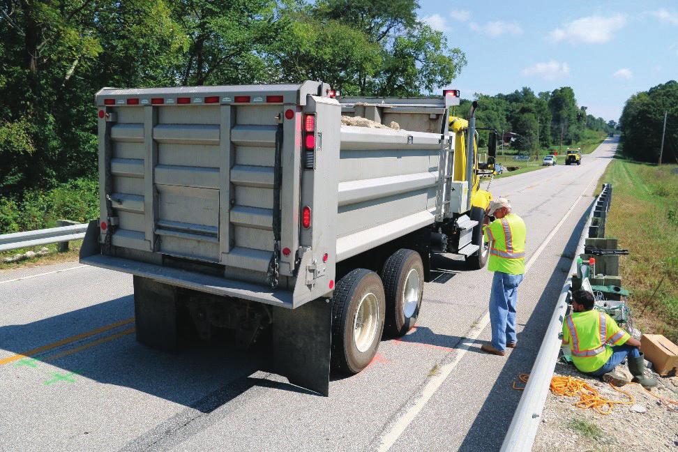
22 TABLE 5.2 Comparison between AASHTO System and the USCS (adapted from Das, 2010) Comparable Soils in USCS AASHTO System Most Probable Possible Possible but Improbable A-1-a GW, GP SW, SP GM, SM A-1-b SW, SP, GM, SM GP N.A. A-2-4 GM, SM GC, SC GW, GP, SW, SP A-2-5 GM, SM N.A. GW, GP, SW, SP A-2-6 GC, SC GM, SM GW, GP, SW, SP A-2-7 GM, GC, SM, SC N.A. GW, GP, SW, SP A-3 SP N.A. SW, GP A-4 ML, OH CL, SM, SC GGM, GC A-5 OH, MH, ML, OL N.A. SM, GM A-6 CL ML, OL, SC GC, GM, SM A-7-5 OH, MH ML, OL, CH GM, SM, GC, SC A-7-6 CH, CL ML, OL, SC OH, MH, GC, GM, SM Note: N.A. 5 Not Applicable. TABLE 5.3 Typical Values of Dry Unit Weight for Different Soils Classified by USCS (adapted from Geotechdata.info, 2016) USCS Description Average Value (pcf) GW Well graded gravel, sandy gravel, with little or no fines GP Poorly graded gravel, sandy gravel, with little or no fines GM Silty gravels, silty sandy gravels GC Clayey gravels, clayey sandy gravels SW Well graded sands, gravelly sands, with little or no fines SP Poorly graded sands, gravelly sands, with little or no fines SM Silty sands SC Clayey sands (Equation 5.1). The pore pressure is calculated by multiplying the column of water times the unit weight of water. The vertical effective stress is obtained by the difference in total vertical stress and pore pressure. For systems that are not saturated the pore pressure becomens zero and the total vertical stress is equal to the effective vertical stress. s v ~s v zu ð5:1þ where, s v is the total vertical stress, s v is the effective vertical stress, and u is the pore pressure. The unit weight of soil is usually obatined from soil sampling and testing. It depends on the soil type and degree of compaction. If the actual weight of earth is unkown, 120 pcf is generally assumed (Ryan et al., 2012). Typical values of soil unit weights can be found in soil mechanics books. Table 5.3 shows typical values of dry unit weight for different soils classified by USCS. Transient loads in flexible buried bridges correspond to vehicular loadings. Depending on the rating method different live load models are applied. The HL-93 loading is used when the bridge is rated by LRFR method. The HS-20 loading is used for rating bridges under the LFR and ASR methods. The MBE (AASHTO, 2011) set forth the cirteria of the different live load models. When evaluating the live load effects on buried structures, AASHTO (2002, 2014) specifications provide guidelines on the methods used to compute the live load effects when soil cover is present. The live loading effects depend on the height of soil cover and the AASHTO specification being followed. For depths of fill of 1 ft. or more, the wheel load is uniformly distributed over a rectangular area with sides equal to to the tire contact area and increased by the live load distributuion factor (LLDF), as per AASHTO LRFD (2014). When areas of several wheel loads overlap the area is defined by the outisde limits of the individual area of a single wheel load. The live load effects may be neglected when the depth of fill is greater than 8 ft. and exceeds the span length. For multiple span bridges the live load effects may be neglected if the depth of fill exceeds the distance inside the face of end walls (AASHTO, 2014). The dynamic load allowance is also a function of the depth of fill and for depths equal to or greater than 8 ft. it becomes negligible, as shown in the following expression (Equation 5.2): IM~33(1:0{0:125D E ) 0% ð5:2þ where, IM (Impact Factor) is the dynamic load allowance; and D E is the minumim depth of earth cover above the structure in ft. In AASHTO SSHB (2002), for depth fills of 2 ft. or more the live load is considered as a concentrated load 14 Joint Transportation Research Program Technical Report FHWA/IN/JTRP-2018/07

23 uniformly distributed over a square area of sides equal to 1.75 times the height of cover. Areas of several concentrated loads that overlap are limited by the outside limits of each individual area, but, the total width of distrbution shall not exceed the total width of the structure s span (AASHTO SSHB, 2002). For single span structures the live load effects may be neglected when the depth of fill is more than 8 ft. and exceeds the span length. For multiple spans the live load effects may be neglected if the depth of fill exceeds the distance between faces of end supports or abutments (AASHTO SSHB, 2002). When the depth of fill is equal to or less than 2ft. the wheel load is distributed to the top of the structure as a concentrated load (ASSHTO SSHB, 2002). The dynamic load allowance decreases from 30% to 10% as the soil cover increases as depicted in Table 5.4. The live load distribution through earth fills is outlined in AASHTO LRFD (2014) and AASHTO SSHB (2002), respectively (see Appendices A and B). The load factors and load modifiers for flexible buried structures based on AASHTO LRFD (2014) are shown in Table Structural Behavior and Ring Compression Theory Spangler was the first to investigate the deflection of flexible pipes. He recognized that a flexible pipe deforms under soil load and generates horizontal soil support (Whidden, 2009). His findings resulted in the development of his Iowa formula in 1941 and became the foundation of flexible pipe design. Originally flawed, the Iowa formula was later modified by Watkins and Spangler in 1958 (Whidden, 2009). The Iowa formula was not intended to be used in design but rather shows the importance of the horizontal soil support on ring deflection. For pipe design the vertical ring deflection ratio is of greater value than horizontal ring deflection (Whidden, 2009). The vertical ring deflection ratio d is approximately TABLE 5.4 Impact Factor for Structures with Soil Cover (adapted from AASHTO SSHB, 2002) Soil Cover IM 0 ft. to 1 ft. 30% 1 ft. 1 in. to 2 ft. 20% 2 ft. 1 in. to 2 ft. 11 in. 10% Note: IM 5 Impact Factor. (and conservatively) equal to the vertical compression strain of the side-fill soil due to the external pressure. For a circular cross-section the assumption of elliptical ring deflection, i.e., the vertical diameter decreases while the horizontal diameter increases, is based on theoretical analysis of a buried pipe in a homogenous, isotropic, elastic medium (Whidden, 2009). The excessive soil compression allows the flexible structure to deflect, thus, a limiting value of 5% of ring deflection ratio was proposed by Spangler. This ratio conforms to NAVFAC (1986). The laboratory confined compression test is typically used to predict the vertical strain of a soil sample and, thus, useful for predicting the ring deflection of a flexible buried structure. However, the side-fill soil under a flexible structure is biaxial while the confined compression test is normally uniaxial. Consequently, the side-fill soil vertical strain under a flexible buried structure is conservatively predicted by the confined compression test (Whidden, 2009). The stress-strain relationship of a coarse soil (little to no fines soil) is a function of the relative density and confined stress. This relationship is illustrated in Whidden (2009), where the secant modulus E is the slope of the stress-strain curve and the ring deflection is a function of the stiffness ratio R s. The ring deflection can be estimated by using the strain-stress and stiffness ratio relationships. An illustrative example can be found in the NAVFAC (1986). Overall, the structural behavior of a flexible buried structure involves in the proper interaction between the soil and structural member (Watkins & Anderson, 1999). The structure and soil attempt to deflect as loads are applied at the top of the embankment. To illustrate this effect, consider a round cross-section that attempts to deflect when vertical loads are applied. In this scenario, the vertical diameter will decrease as the horizontal diameter increases. The increase in the horizontal diameter is resisted by the lateral soil pressure. However, if no proper interaction between the soil and the structural member exists, then the cross-section deforms appreciably resulting in unrecoverable deformations. Whether a good compacted material is used or not plays an important role in the behavior of flexible structures. This behavior can be considered during field inspections. Thus, if no signs of significant distress or deformation is found during a field assessment, it is reasonable to assume that a proper backfill material was provided during installation. TABLE 5.5 Load Factors and Load Modifiers for Flexible Buried Structures (adapted from Michael Baker, Inc., 2007) Dead Load Earth Load Live Load Bridge Type c max c min g c max c min g c max g Corrugated metal pipe or arch Corrugated metal box Plastic pipe (HDPE or PVC) Joint Transportation Research Program Technical Report FHWA/IN/JTRP-2018/07 15

24 Traditionally, flexible buried structures have been designed using the Ring Compression Theory (RCT). The RCT is an approach that suggests that a flexible structure can be analyzed as a thin ring in compression when installed in a well compacted backfill material. This theory assumes that the non-uniform soil pressure distribution around the structure has little effect on the magnitude and distribution of the circumferential thrust (Yeau, 2010) and, thus, simplifying the complex loading conditions on a flexible structure by assuming a uniform pressure distribution. The use of the RCT is valid for flexible circular sections where the depth of fill exceeds one-eighth of the pipe diameter (Yeau, 2010) or one-quarter its diameter (Howes, 1964). The uniform pressure is taken as the overburden pressure of the soil plus any distributed live load effect. Thus, based upon the RCT, the circumferential thrust in the pipe wall can be found by the following expression (Equation 5.3): T~P S ð5:3þ 2 where, T is the circumferential thrust; P is the uniform pressure on top of the structure; and S is the diameter of pipe or span of plate structure. For a non-circular cross-section, such as a pipe-arch (Figure 5.1), the radial soil pressure varies such that the circumferential thrust remains constant throughout the circumference (Yeau, 2010). For this type of crosssection the soil pressure on the structure at any given point can be found by Equation 5.4. Overall, for any flexible bridge-size culvert shape, its design is achieved by providing adequate wall area such that the thrust does not exceeds the wall strength (NAVFAC, 1986). P~ T R ð5:4þ where, R is the radius of curvature at the point under consideration; i.e, R t 5 radius of curvature at top of arch; R b 5 radius of curvature at bottom of arch; and R h 5 radius of curvature at haunch of arch. would resist the applied dead and live load effects and the flexibility limit. The flexibility limit is required so that the flexible structure can be properly handled, installed, and backfilled. The flexibility limit is defined by the flexibility factor (FF) of the structure, where FF is expressed using the following expression (Equation 5.5): FF~ S2 E m I ð5:5þ where, E m is the modulus of elasticity of metal; I is moment of inertia per unit length of cross-section; and S is the diameter or maximum span. The intention of a FF is to measure the rigidity of the flexible structure during installation. This allows the structure to resist the deformation or buckling during the backfill operation or transportation Strength Limit States for Flexible Buried Structures The strength limit states for this type of structures are governed by the thrust capacity. Both the AASHTO LRFD (2014) and AASHTO SSHB (2002) adopt the RCT in designing flexible buried structures. Overall, the thrust capacity is determined as the lowest of the factored wall area, buckling strength and seam resistance. Wall Area. The wall strength of flexible buried structures is governed by the following expression (Equation 5.6): jr n ~jf y A ð5:6þ where, R n is the wall yield strength per linear foot; f y is the specified minimum yield point; A is the wall area per linear foot; and j is the resistance factor. Buckling Strength. When the the critical buckling stress is less than the specified yield point the wall strength needs to be recalculated as shown in the following expressions (Equation 5.7, Equation 5.8, and Equation 5.9): Thrust and Flexibility Limits Overall, the design of flexible structures is achieved by the compressive strength or thrust capacity that jr n ~jf cr A sffiffiffiffiffiffiffiffiffiffiffi f cr ~f u { f u 2 (ks=r) 2 if Sv r 24E m 48E m k f u sffiffiffiffiffiffiffiffiffiffiffi f cr ~ 12E m (ks=r) 2 if S r 24E m k f u ð5:7þ ð5:8þ ð5:9þ Figure 5.1 Pipe-arch cross-section. where, f cr is the critical buckling stress; f u is the tensile strength of metal; k is the soil stiffness factor; and r is the radius of gyration of corrugation. A value of k50.22 is recommended by AASHTO LRFD (2014) and AASHTO SSHB (2002). The stress and length values, when used in the above expressions, are input in ksi and in., respectively. 16 Joint Transportation Research Program Technical Report FHWA/IN/JTRP-2018/07

25 TABLE 5.6 List of Variables for MPA-UF Variable Description A D bolt d E m f cr f y f u H I k p N bolt R bolt R S t c s Area of corrugated cross-section per linear foot Bolt diameter Depth of corrugation Modulus of elasticity of metal Critical buckling stress Specified yield point stress Specified minimum tensile strength Depth of earth cover Inertia of cross-section per linear foot Soil stiffness factor Pitch length Number of bolts per linear foot of longitudinal seam Bolt shear capacity per linear foot of longitudinal seam Radius of gyration of cross-section Maximum span Plate thickness Unit weight of backfill Figure 5.2 Arranged bolt pattern in longitudinal seam. Seam Resistance. For bolted structural steel plate the factored resistance of the seam needs to be sufficient to develop the factored thrust in the pipe wall. If no seam is utilized, then this limit does not need to be considered. The seam strength is given by the following expression (Equation 5.10): jr n ~jr bolt N bolt ð5:10þ where, N bolt is the number of bolts in one linear foot; and R bolt is the bolt shear capacity per linear foot Summary of MPA-UF Characterization After conducting the bridge characterization it was found that the critical information needed in the bridge load rating process of flexible buried structures are the corrugation size, presence of longitudinal seam, height of fill, and material properties. A list of variables required for the load rating calculations is presented in Table Field Survey and Inspection Field measurements were collected to update the missing information of the MPA-UF structure in consideration. It was found that the bridge was built with a SSP with 6 x 2 in. corrugations and thickness of in. The thickness of the plate was measured using a digital caliper at several locations and averaged. The pitch and depth were measured using a measuring tape at several locations and averaged. The longitudinal seam utilized four bolts per linear foot with bolt diameter of L in. in each of the three barrels comprising the structure. Figure 5.2 shows the bolt pattern present in the seam. Each barrel is a 92 in. diameter circular pipe and the distance between themwas49in.themeasurementsweremadeusinga measuring tape. Figure 5.3 Measurement of depth of soil cover. The depth of fill was measured using a level and a level rod (Figure 5.3) and it was estimated to be 11.3 ft. The elevation of the fill should be measured where the maximum live loading is applied. This location usually corresponds to the roadway above the flexible structure. Because of the difficulty in placing the level rod in the middle of the roadway due to the upcoming traffic, locations such as the shoulders were used in lieu of the center of the roadway. The difference in elevation between the top of the barrel and roadway resulted in the height of the fill. No signs of distress or excessive deformation were observed during the field inspection. It was assumed that typical standards for installation and construction of standard flexible buried structures were followed by a competent engineer. Thus, the backfill material was assumed to be a well compacted material following AASHTO specifications. Drawings of the bridge-size culvert over US 24 were created using the information collected from the Joint Transportation Research Program Technical Report FHWA/IN/JTRP-2018/07 17

26 Figure 5.4 Corrugated steel arch plan view, cross-section elevation, and corrugation size. database and field measurements. The drawings included a plan and typical cross-section views, and details of the corrugation size (Figure 5.4). 5.3 Load Rating The measured corrugation size and plate thickness were compared with standard corrugation sizes found in AASHTO specifications. It was found that the measured corrugation size matched those specified in standard tables containing the section properties for different corrugation sizes used in standard SSP design. Thus, the section properties were obtained from the standardized section properties tables. Table 5.7 shows the section properties for different plate thickness for 6 x 2 in. corrugations. The mechanical properties of SSP were based upon ASTM A761 (Table 5.8). The corrugation, i.e., pitch and depth, measured for as-built structures usually match those found in standardized tables. However, the thickness of the plate might present section loss due to corrosion or loss of coating. For those cases, standardized section properties tables might not be suitable for obtaining the section properties of the actual corrugation. Instead, the section properties can be computed using actual corrugation dimensions. Alternatively, the standardized section properties that closely matched those measured in the site can be used in conjunction with a resistance factor to account for section loss when checking the strength limits. The provisions found in the AASHTO (2002, 2014) specifications and CONTECH (2015) were used to discern the seam requirements. SSP pipes are typically designed using four bolts per foot of longitudinal seam (CONTECH, 2015). The seam resistance is usually the limiting factor when the depth of fill is significant TABLE 5.7 Cross-Section Properties of Steel Structural Plate (adapted from AASHTO, 2002, 2014) 6 x 2 in. Corrugations t (in.) A (in. 2 /ft.) R (in.) I (in. 4 /in. x 10-3 ) a a Measured plate thickness during field assessment. TABLE 5.8 Mechanical Properties for Design of Steel Structural Plate (adapted from AASHTO, 2002, 2014) f u (ksi) f y (ksi) E m (ksi) ,000 (CONTECH, 2015). For such cases, the standard four bolt per foot of seam may not be sufficient to resist the applied loads. Thus, the designer may consider six or eight bolts per foot of seam. The use of four bolts per foot of seam having L in. diameter and meeting ASTM A449 are typical in SSP design and installation. This four bolt per foot of seam configuration was observed during the field inspection. It was assumed that the bolts installed on the structure follow typical standards for SSP. Thus, the minimum 18 Joint Transportation Research Program Technical Report FHWA/IN/JTRP-2018/07

27 requirements of longitudinal seam strength specified in AASHTO specifications were conservatively assumed. Table 5.9 shows the minimum longitudinal seam strength for 6 x 2 in. corrugations used in design for bolted SSP pipe, pipe-arch, and arch. The National Corrugated Steel Pipe Association (NCSPA, 1995) addresses the load rating of corrugated steel structures based upon the AASHTO SSHB (2002) and the LFR method. The rating is governed by the thrust capacity, which is the lowest between the wall area, buckling strength, and seam resistance, and minimum cover requirements (NCSPA, 1995). Yeau (2010) recognized that the minimum cover requirements is independent of pipe material, plate thickness, and loading conditions. Because of these shortcomings, a rating based on minimum cover requirements does not reflect any change in the load rating of the structure when it has experienced section loss due to corrosion or damage due to loading and environmental conditions. Thus, Yeau (2010) proposed that the minimum soil cover requirements should not be considered as a load rating check, but, it does need to be satisfied to ensure the structure stability. Minimum soil cover values based on the critical pressure that will cause instability in the structure were reported by Yeau (2010). Yeau and Sezen (2012) proposed a load rating procedure for corrugated metal culverts. The procedure is similar to the one recommended by NCSPA (1995) but included new capacity reduction factors for wall area and seam resistance based upon different appraisals for the wall and seam during annual inspections. Additionally, the effect of external live load is not included in the proposed load rating procedure for deep bridgesize culverts and for culverts subjected to low live load stresses (Yeau & Sezen, 2012). The reduction factors for wall and seam reflect the current condition of exiting flexible structures. The factors are based upon a general appraisal number of the inspected condition of the wall area and seam during regular inspections. An appraisal number N equal to 0 represents the worst damage or failure condition and a value of 9 indicates the best possible condition (Yeau & Sezen, 2012). The values of the reduction factors for seam resistance and wall area can be found in the paper by Yeau and Sezen (2012). If a flexible structure experienced permanent deformations during or after construction, the load rating is assigned based upon the change in the culvert deflection rate (Yeau & Sezen, 2012). This change affects the buckling strength. The deflection ratio d is used to reduce the buckling strength of the flexible structure when it has vertical deflection or flattening at the crown. However, local buckling and associated deflections do not necessarily occur at the crown (Yeau & Sezen, 2012). A new factor was introduced to account for local buckling, which is defined as the ratio of change in top radius. The proposed new buckling factor by Yeau and Sezen (2012) can be calculated using the following expression (Equation 5.11): 8 >< 1:0 for no deflection or buckling j bkl ~ 0:95{5:6d for deflection at the crown ð5:11þ >: 0:95{4:6 m R t for local buckling where, m is the measured ordinate; R t is the measured top radius of arch; and d is the deflection ratio. The load rating of Bridge No was similar to the one recommended by NCSPA (1995) and Yeau and Sezen (2012). For flexible buried structures the load effect due to the wearing surface load is usually not significant, especially when the depth of fill is substantial. Additionally, the load rating is mainly controlled by the thrust capacity. The general load rating equation for the LRFR and LFR methods can then be simplified using the following expressions (Equation 5.12 and Equation 5.13), respectively: RF~ j c j s C{g EVc EV T EV g LL c LL (T LL zim) ð5:12þ where, j c is the condition factor; j s is the system factor; C is the thrust capacity; g EV is the load modified for earth loads; g LL is the load modifier for live loads; c EV is the load factor for vertical earth load effect; c LL is the TABLE 5.9 Minimum Longitudinal Seam Strengths (adapted from AASHTO, 2002, 2014) t (in.) Bolt Diameter (in.) 4 Bolts/ft. (kip/ft.) 6 Bolts/ft. (kip/ft.) 8 Bolts/ft. (kip/ft.) / N.A. N.A a 3/4 b 62.0 N.A. N.A / N.A. N.A / N.A. N.A / N.A. N.A / N.A. N.A / /8 N.A. N.A /8 N.A. N.A Note: N.A. 5 Not Applicable. a Measured plate thickness during field assessment. b Assumed bolt diameter during field assessment. Joint Transportation Research Program Technical Report FHWA/IN/JTRP-2018/07 19

28 TABLE 5.10 Load Rating Results of Bridge No Rating Method Inventory RF Operating RF Service RF LRFR LFR load factor for live load effect; T EV is the thrust due to the vertical earth load effect; T LL is the thrust due to the live load effect; and IM is the dynamic load allowance. RF~ C{A 1T EV A 2 (T LL zim) ð5:13þ where, C is the thrust capacity; A 1 is the load factor for earth load effect; A 2 is the load factor for live load effect; T EV is the thrust due to the vertical earth load effect; T LL is the thrust due to the live load effect; and IM is the dynamic load allowance. The load rating calculations were performed based upon the LRFR and LFR methods (see Appendix C). Table 5.10 shows the load rating results. The results showed that the live load effect was significantly dissipated through the earth fill and reaching the structure with lower stress levels. Hence, the values obtained for the RFs were relatively high. The LRFR method resulted in more conservative ratings than the LFR method for the MPA-UF on US CASE STUDY BRIDGE NO This section demonstrates the application of the proposed general procedure on a RCA-UF structure without plans. This section provides a detailed review of the step-by-step process included in the general procedure. 6.1 Bridge Characterization This bridge carries SR 45/SR 58 over a branch of Doan s Creek and will be referred herein as the Doan s Creek Bridge. It was categorized as a RCA-UF based upon the observations made during the second field assessment. A literature review of earthen-filled concrete bridges was conducted as part of the general procedure under the bridge characterization process. A review of the literature is presented in the following subsections Rigid Buried Structures The backfill material on buried structures corresponds to the compacted soil placed during construction around a structural member. The structural member can have different shapes and is mainly made of reinforced concrete (cast-in-place or precast). Buried structures made of concrete or stone masonry are defined as rigid because they are very stiff and do not deflect appreciably under external loading. While the soil-structure interaction is critical to develop the load-carrying capacity of flexible buried structures, this is not often the case in rigid buried structures. Instead, the load-carrying capacity is mostly provided by the structural member itself (Ryan et al., 2012) Materials and Shape Types of buried concrete bridges include box, pipe, arch, and frame. Concrete box structures are one of the most common rigid buried structures used today (Ryan et al., 2012). They have an integral bottom slab that supports the side walls and top slab forming a channel opening for the water flow. The box opening is determined by the site constraints as well as the hydraulic, geotechnical, and structural design criteria. A multi-cell box can be used to accommodate longer spans. It is important to note that although a box structure may have multiple barrels, it is still a single structure. The internal walls are provided to reduce the unsupported length of the top slab. The primary members of a concrete box bridge are the top slab, bottom slab, and sidewalls (Ryan et al., 2012). In cases where there is no bottom slab, the structure is referred to as a concrete frame bridge. Concrete pipe structures are commonly made of precast concrete and manufactured in three standard shapes: circular, horizontal elliptical, and vertical elliptical. The circular shape is the most common shape manufactured for pipe concrete structures. They are hydraulically and structurally efficient under most conditions. Elliptical shapes are used in situations where horizontal or vertical clearance is limited. When the size of the opening for the water flow is very large, two or more concrete pipe structures may be used. A concrete arch bridge has a curved-shape (circular or parabolic) member that works primarily in compression and does not have a horizontal floor like a concrete box. The arch member is supported by abutments or piers. The heels and crown are the lowest and highest points of the arch, respectively. A horizontal distance between two heels is the span, and the vertical distance between the heel line and crown is the rise. A variation of the arch bridge is the tied arch bridge. It is basically the same as the arch bridge, but it has an integral floor serving as a tie between the ends of the arch (Ryan et al., 2012). Concrete arch structures are either cast-inplace or precast. The internal forces resisted by the arch member are the bending moment, shear, and axial force (Karnovsky, 2012) Loads Rigid buried structures are subjected to permanent and transient loads. The basic permanent loads applied in the design of a rigid structure include dead loads, vertical and horizontal earth pressure. The dead load includes the structure self-weight, wearing surface loads, and any other additional external dead load. The vertical earth pressure is produced by the weight of the soil fill. The horizontal earth pressure is related to the vertical earth pressure by a lateral earth coefficient. 20 Joint Transportation Research Program Technical Report FHWA/IN/JTRP-2018/07

29 There are three categories of lateral earth pressure and each depends upon the movement experienced by the wall on which the pressure is acting. The three categories are at-rest earth pressure, active earth pressure, and passive earth pressure. Walls that can tolerate little or no movement should be designed for at-rest earth pressure (AASHTO, 2014). Walls which can move away from the soil mass should be designed for pressures between active and at-rest conditions, depending on the magnitude of the tolerable movements (AASHTO, 2014). If the wall moves into the soil mass, then the soil mass is compressed, which mobilizes its shear strength and the passive earth pressure develops. The lateral earth pressure is found by the following expression (Equation 6.1): p~kc s z ð6:1þ where, p is the lateral earth pressure; k is the coefficient of lateral earth pressure (at-rest, active, or passive); c s is the unit weight of soil; and z is the depth below the surface of earth. The resultant lateral earth load due to the weight of the backfill is assumed to act at a height of H/3 above the base of the wall, where H is the total wall height, measured from the surface of the ground at the back of the wall to the bottom of the footing (AASHTO, 2014). The coefficient of lateral earth pressure is taken as k o for walls that do not deflect or move, k a for walls that deflect or move sufficient to reach minimum active conditions, or k p for walls the deflect or move sufficiently to reach a passive condition (AASHTO, 2014). Since soil backfill for these types of buried structures is typically granular material such as sand, silty sand, sand with gravel, as specified in AASHTO specifications, this subsection discussion is based upon coarsegrained, non-cohesive soils. However, there are many textbooks and other publications where this topic is fully discussed. The coefficient of at-rest lateral earth pressure in granular, normally consolidated soils may be taken as (Equation 6.2): k o ~1{ sin w f ð6:2þ where, w f is the effective friction angle of soil; and k o is the coefficient of at-rest lateral earth pressure. Depending upon whether the soil is loose or dense, there are published relationships that depend upon the soil s engineering values for calculating at-rest lateral earth pressure. There are two relatively simple classiscal theories (among others) that are widely used when discussing active and passive lateral earth coefficients. These theories are the Rankine and Coulomb earth pressure theories. The Rankine theory assumes there is no friction between the wall and soil and assumes that the lateral pressure is limited to vertical walls. The Coulomb theory assumes friction between the wall and soil and is not limited to vertical walls. Another difference between the theories is that Rankine theory assumes that the lateral resulant force is parallel to the top surface of the backfil while in the Coulomb theory the resultant force is not necessarily parralel to the backfill surface because of the soil-wall friction value. The general expression of the Rankine active and passive lateral earth pressure coefficient is a function of the effective internal friction angle of soil and slope angle of backfill. The Rankine active and passive lateral earth coefficient for the specific condition of a horizontal backfill surface is calculated as follows (Equation 6.3 and Equation 6.4): k a ~ 1{ sin w f 1z sin w f ð6:3þ k p ~ 1z sin w f 1{ sin w f ð6:4þ The Coulomb active and passive lateral earth coefficient is derived from a more complicated expression that depends on the effective friction angle of soil, the angle of the back of the wall, the soil-wall friction value and the slope angle of backfill. Although this expression is not shown, these values are readily available in textbook tables. The general cases for calculating earth pressure coefficients can be found in published expressions, tables, and charts for the various conditions such as wall friction and sloping backfill. The reader should obtain these coefficients from published sources for conditions other than those discussed herein. The transient loads in rigid buried structures correspond to vehicular traffic. Depending on the rating method different live load models are applied. The criteria set forth for the live load models and their distribution through earth fills is found in AASHTO specifications and are the same as those discussed in flexible buried structures (see Section 5.1.4). The load factors and load modifiers for rigid buried structures based on AASHTO LRFD (2014) are shown in Table Strength Limit States for Rigid Buried Structures The general strength limit states for this type of structures are governed by flexure, shear, thrust, and radial tension, depending on the type of rigid buried structure. For precast concrete pipes the safety against structural failure is determined by flexure, thrust, shear, and radial tension limit states. For reinforced concrete cast-in-place and precast box, and reinforced cast-inplace arch the safety against structural failure is determined by flexure, axial, and shear limit states. For a reinforced concrete arch, as the Doan s Creek Bridge, that primarily works in compression and is generally subjected to some degree of flexure, the combined action of both forces may be the controlling strength limit state. An interaction diagram is useful for the design of compression members subjected to flexure but has theoretical and analytical limitations in their use for Joint Transportation Research Program Technical Report FHWA/IN/JTRP-2018/07 21

30 TABLE 6.1 Load Factors and Load Modifiers for Rigid Buried Structures (adapted from Michael Baker, Inc., 2007) Dead Load Earth Load Live Load Bridge Type c max c min g c max c min g c max g Reinforced concrete pipe Reinforced concrete box Reinforced concrete arch TABLE 6.2 List of Variables for RCA-UF Variable Description A bh A s Area of tension reinforcement A s Area of compression reinforcement A v Area of transverse reinforcement c.c. Clear concrete cover b Width of arch barrel d Distance from extreme compression fiber to centroid of tension reinforcement d Distance from extreme compression fiber to centroid of compression reinforcement E c Modulus of elasticity of concrete E s Modulus of elasticity of reinforcement f Rise f c Compressive strength of concrete f y Yield strength of steel reinforcement h Height of arch barrel H Depth of earth cover over crown l Clear span s Spacing of principal reinforcement s v Spacing of transverse reinforcement c c Unit weight of concrete c s Unit weight of backfill k Lateral earth coefficient w f Effective friction angle of backfill load rating because the value of the capacity of the member depends upon the unknown load. Ranasinghe and Gottshall (2002) proposed an iterative load rating method for the evaluation of compression members subjected to flexure. This method was adopted to load rate the Doan s Creek Bridge Summary of RCA-UF Characterization After conducting the bridge characterization it was found that the critical information needed in the bridge load rating process of reinforced concrete arch bridges with soil cover are geometric data, material properties, among other parameters (Table 6.2). 6.2 Bridge Database Past and current inspection reports were located for the Doan s Creek Bridge. Routine inspection reports for the years 2008, 2010, 2012, 2014, and 2016, as well as two underwater investigation reports from 1997 and 2003 were provided by INDOT. The reports showed that the Doan s Creek Bridge was built in An underwater inspection that consisted of a visual and tactile examination of the accessible substructure surface from the waterline to the channel bottom conducted on July 11, 1997 revealed that the foundation consisted of spread footings with no piles. The condition of the abutments and pier was described as generally in good condition as of 1997 and changed to generally fair condition with no structurally significant defects based on the underwater inspection performed on October 9, Based on the routine inspection reports this bridge was initially considered to be scour critical. In November 2010 scour countermeasures were installed and since then no scour related deficiencies have been observed as noted in the inspection reports. According to the routine inspection reports the arch was in good condition as of 2002 but longitudinal cracks at the intrados were reported in In 2014 the previously noted cracks presented minor efflorescence and it was reported that the headwall of the west span was replaced as part of a rehabilitation contract. 22 Joint Transportation Research Program Technical Report FHWA/IN/JTRP-2018/07

31 No specific date was noted for the replacement work and no plans for the rehabilitation contract were located. Moderate efflorescence at interior haunch of both spans was reported in the last inspection report, which rated the arch with a NBI condition rating equal to 6, i.e., deterioration or initial disintegration. Lastly, no rating analysis or evaluation was reported by any of the inspection reports. A search for comparable bridge plans was conducted based on the year of original construction of the Doan s Creek Bridge. The search for plans was performed using the Indiana Bridge Inspection Application System (BIAS). The BIAS is a software platform use for entering and retrieving bridge inspection related data. The search was filtered for RCA-UF type and state-owned bridges that ranged from 1940 through Forty-five bridges matched the search, but only twenty-two bridges contained comparable plans on file. All comparable plans showed one-span reinforced concrete arch bridges with span length varying from 25 ft. to 40 ft. The rise varied from 7 ft. to 15 ft., and the depth of soil cover ranged from 1.3 ft. to 13.3 ft. Some of the plans had design data notes that specified the unit working stress of concrete and design live load as either H-20 or HS-20 truck loading as in accordance with AASHO SSHB (1941, 1944). The design philosophy corresponding to that era was the Allowable Stress Design (ASD). The majority of plans showed that single arch bridges were supported over spread footings with no piles. A data sheet was found in Indiana BIAS with the detailing of the pier where two arches coincide. The data sheet also showed that the pier was supported by spread footings with no piles. It was assumed that the Doan s Creek Bridge pier has a similar detailing. Based on the information collected from comparable plans, it was found that the arch barrels were typically detailed with two layers of primary longitudinal reinforcement (parallel to span) and two layers of secondary longitudinal reinforcement (transverse to span). The clear concrete cover was 2 in. for all plans as in accordance with AASHO SSHB (1941, 1944) and the transverse reinforcement was provided along the arch barrel using single leg stirrups. The spacing of the longitudinal and transverse reinforcement was the same in all plans irrespective of the bar size. The spacing was 12 in. for the primary longitudinal reinforcement and 24 in. for the secondary longitudinal and transverse reinforcement. The primary reinforcement for the top and bottom layer was the same within each plan and varied between rebar sizes of # 4, # 5, and # 6(A s , 0.31, and 0.44 in. 2, where A s is the area of tension reinforcement). The secondary and transverse reinforcement was # 4 for all plans. The rebar size # 5 accounted for 68% of the bridge population. The arch thickness in the comparable plans varied between 8 in., 9 in., and 10 in., where 9 in. constituted about 55% of the bridge population. In addition, the year of construction, location of bridge, reinforcement ratios per linear foot for top, bottom and total reinforcement, distance from extreme tension fiber to centroid of tension reinforcement, and distance from compression fiber to centroid of compression reinforcement were reviewed in the comparable plans to create a database. A condensed bridge database highlighting some of the critical bridge information found in the comparable plans is shown in Table Field Survey and Inspection Field measurements were made to supplement the additional information needed to characterize the Doan s Creek Bridge. The measurements showed that the bridge is comprised of two arches with a clear span of 11.5 ft. and a rise of 5.75 ft. The observations made during the field survey as well as the measured span and rise indicated that both arches have a semi-circular shape. The height of soil cover was measured using a level and level rod and it was 3.42 ft. on both sides of the road. This measurement was referenced from the coping to the shoulders of the road surface in lieu of the center of the road. The shoulder were used as reference because of the difficulty in placing the level rod over the center of the road due to the oncoming traffic. The depth of soil cover over the crown was estimated based upon the thickness and measured depth of fill over the shoulders. The arch thickness was not measured since access to it was denied because the arch barrel is within the headwalls. The thickness was estimated based upon the arch thickness found in the bridge database of comparable plans. Additional field measurements, such as wingwall dimensions, roadway width, among other measurements, were obtained to complete the geometry of the Doan s Creek Bridge. The field inspection (Figure 6.1) did not reveal any new information aside from what the inspection reports already noted. Overall, no signs of significant distress or deterioration were encountered during the field inspection. Because of the general good condition of the structure it was assumed that typical standards for installation and construction of reinforced cast-in-place arches and backfill material followed the AASHTO/ AASHO specifications. Drawings of the Doan s Creek Bridge were created using the information collected from the database and field measurements. The drawings included a plan and typical cross-section view (Figure 6.2). The reinforcement configuration and arch thickness were adapted from the bridge database of comparable plans. Although it was discerned that the foundation was supported by spread footing with no piles, field measurements of the foundation were not possible due to the inaccessibility nor did the underwater inspection reports show any dimensions of the footings. Joint Transportation Research Program Technical Report FHWA/IN/JTRP-2018/07 23

32 TABLE 6.3 Database of Survey of Comparable Plans Bridge Number Year Built l (ft.) f (ft.) H (ft.) h (in.) A s (in. 2 ) a A A a a (231) (231) I A A A A a A Note: l 5 clear span; f 5 rise; H 5 depth of soil cover; h 5 arch thickness; A s 5 area of tension reinforcement. a Different comparable plan with same bridge number. Figure Load Rating Field inspection of the northeast arch. The concrete compressive strength and rebar yield strength were estimated as 3,000 psi and 33,000 psi, respectively. The concrete compressive strength and rebar yield strength estimation was based on the unit working stress specified in the design data notes found in the comparable plans and AASHO SSHB (1941, 1944). For concrete structures, AASHO (1941) specifies a unit working stress of 1,000 psi for concrete members in compression. This value, also specified in the design data notes of comparable plans, was based on the use of concrete having an ultimate compressive strength at 28 days of 3,000 psi. Thus, it was assumed that the Doan s Creek Bridge was designed using a concrete compressive strength of 3,000 psi. The unit working stress for reinforcing steel is specified as 18,000 psi as per AASHO (1941). Based on AASHO (1941), the unit working stress of steel reinforcement can be assumed to be of the yield point. The rebar yield stress was then estimated by dividing the unit working stress by The computed yield point of 33,000 psi was in accordance with MBE 6A and 6B (AASHTO, 2011). Two arch cross-sections for an earthen-filled reinforced concrete arch were idealized based on the information discerned from the survey of comparable plans. The first doubly reinforced cross-section contained a # 5 rebar size and 9 in. thickness. The second crosssection had a # 4 rebar size and 8 in. thickness. The latter cross-section was conservatively assumed for the load rating calculations. It was found that a simplified load rating evaluation was suitable for the Doan s Creek Bridge since the critical bridge information presented in Table 6.2 was obtained by measurements or inferred from comparable plans and past standards. The load rating calculations began by computing the dead loads, earth loads, and live load on a 1 ft. wide section of the arch. The dead loads included the distributed self-weight of the arch and the earth loads were calculated as distributed loads due to the self-weight of the soil fill. The arch selfweight was based on a concrete unit weight of 150 pcf as per AASHO (1941). The unit weight of soil placed on top of the arch was taken as 120 pcf as per AASHO and 2.2 (1941). The vertical earth pressure acting on top of the structure was computed based 24 Joint Transportation Research Program Technical Report FHWA/IN/JTRP-2018/07

33 Figure 6.2 Doan s Creek Bridge: (a) plan view; (b) cross-section elevation. on the principles of soil mechanics and obtained by multiplying the unit weight of soil times the depth of soil cover. A coefficient of lateral earth pressure of 0.5 was used for the earth lateral pressure on the assumption that the structure can tolerate little to no movement as per AASHTO SSHB (2002). This coefficient was based on an at-rest condition and an effective friction angle of 30u as per AASHTO Table 5.5.2B (2002). Equation 6.2 was used to calculate the lateral earth coefficient at-rest condition. Live loads were caused by an HS-20 truck driving over the bridge. Seven different live load combinations were produced by moving the truck axles over the length of the bridge. Each combination was calculated as per AASHTO SSHB 6.4 (2002) for the distribution of wheel loads through earth fills. i.e., when the depth of fill is 2 ft. or more, concentrated loads are considered as uniformly distributed over a square with sides equal to 1.75 times the depth of fill (AASHTO SSHB, 2002). No impact effects were considered as the impact factor for structures with fill equal to or greater than 3 ft. is negligible. The Doan s Creek Bridge was modeled using the commercially available structural analysis and design software SAP2000 (Version ). A simplified model of the bridge was created, where each arch was divided Joint Transportation Research Program Technical Report FHWA/IN/JTRP-2018/07 25

34 into several portions and each curvilinear portion was approximated by a straight member of equal length. The frame element is a straight line that connects two nodes and uses a general, three-dimensional, beamcolumn formulation which includes the effects of biaxial bending, torsion, axial deformation, and biaxial shear deformation (CSi, 2016). This type of element was used to represent the arch member and each arch was modeled using 180 frame elements. The model was loaded with the calculated dead, earth, and live loads. The model contained 362 values of axial, shear and bending moment for each load case (dead, earth, and live loads). These values were reduced to half because of the bridge symmetry. Figure 6.3 Section forces diagram for east span: (a) factored axial force; (b) factored bending moment; (c) factored shear force. 26 Joint Transportation Research Program Technical Report FHWA/IN/JTRP-2018/07

35 The boundary condition at the supports was assumed as a two-hinged (pinned) and hingeless (fixed) arch configuration to determine the maximum demand acting along the arch. The factored section forces, based on a Load Factor Design (LFD) philosophy, along the arch length of half the structure are shown in Figure 6.3. The x-axis represents the angle h in degrees measured clockwise with respect to the center of the semi-circle, e.g., 0u represents the east abutment support and 90u represents the crown. The arch was evaluated for the strength limit state and found that the combined action of axial compression and flexure was the controlling limit state. An iterative load rating procedure (Ranasinghe & Gottshall, 2002) was adopted for the load rating of the Doan s Creek Bridge. The iterative load rating used the equations derived by Wang and Salmon (1985) for the tension- and compression-controlled regions of the interaction diagram (see Appendix D). The iterative process to find the load rating values along the arch length assuming a two-hinged and hingeless arch configuration was automated using the numerical computing software Matlab (Version R2016a) (see Appendix E). The capacity of the member depends upon the unknown load (axial compression and bending moment) and so does the rating factor (RF). The solution is attained when the unknown load in terms of RF is incremented until reaching a point along the curve of an interaction diagram (Figure 6.4). Each point along the curve of an interaction diagram represents a unique value of eccentricity. Thus, an interaction diagram is constructed by a series of values of eccentricity. The automated load rating consists in incrementing the unknown load in terms of the RF and computing the eccentricity. The eccentricity was input into the tension- and compression-controlled equations (Wang & Salmon, 1985) to obtain the member capacity for that value of eccentricity. The section is compressioncontrolled for values of axial load greater than or equal to the balanced load; tension-controlled for values of axial load less than the balance load. The capacity is compared to the initial unknown load and the RF is incremented if the difference between capacity and demand is positive, i.e., the unknown load falls inside the interaction diagram. As the RF is incremented a new value of axial compression load and bending moment is obtained along with a new value of eccentricity. Iterations are repeated until the difference between capacity and demand is negative, i.e., the unknown load falls outside the interaction diagram. A flowchart of the automated load rating process is depicted in Figure 6.5. The load rating calculation followed the LFR method. The RF was incremented by 0.01 from 1.0 until convergence. The controlling Inventory Rating Factor (IRF) when assuming a two-hinged arch configuration was 3.27 and was located at the crown. The controlling IRF when assuming a hingeless arch configuration was 3.72 and was located at the east end support. The Operating Rating Factor (ORF) was 5.45 and 6.20 for the two-hinged and hingeless arch, respectively (Table 6.4). Figure 6.4 Illustrative example of iterative process for computing the rating factor (RF) using an interaction diagram. (Note: e 5 eccentricity; M n 5 nominal moment capacity; P b 5 balanced load; P n 5 nominal axial capacity; DRF 5 rating factor increment.) Joint Transportation Research Program Technical Report FHWA/IN/JTRP-2018/07 27

36 Figure 6.5 Flowchart of iterative load rating process using an interaction diagram. 28 Joint Transportation Research Program Technical Report FHWA/IN/JTRP-2018/07

37 Results were validated by plotting on the interaction diagram the factored axial compression load and bending moment using their respective inventory rating factor based on a concrete compressive strength of 3,000 psi (Figure 6.6). Although a compressive strength of 3,000 psi was justified, the load rating was also investigated assuming a concrete compressive strength of 2,500 psi the minimum value per MBE (AASHTO, 2011). This resulted in values of IRFs of 3.22 and 3.62 for two-hinged and hingeless arch configuration, respectively. The engineer can use judgment on which value to use for the concrete compressive strength Experimental Load Test An experimental load test was performed on the Doan s Creek Bridge to investigate the use of higher levels of evaluation as proposed in the general procedure under the bridge load rating. The instrumentation included strain gage installation along the bottom surface of the east arch. Concrete strain gages with three pre-attached lead wires were used for compensation of temperature induced resistance changes in the strain gage circuit. Shielded wires were used for splicing to minimize the noise effect. All gages were coated to prevent damage form the environment and the lead wires were connected to a data logger unit to record the strain measurements. Two three-axle dump trucks were used for the experimental load test and are referred herein as Truck A TABLE 6.4 Load Rating Results of Bridge No Arch Configuration Inventory Rating Factor Operating Rating Factor Two-hinged Hingeless and Truck B. The weight of Truck A was 60,720 lbf when fully loaded. The weight of the front axle was 12,080 lbf and the weight of the tandem axle was 48,640 lbf. The weight of Truck B was 59,300 lbf when filled with sand. The weight of the front axle was 11,720 lbf and the weight of the tandem axle was 47,580 lbf. For both trucks, the longitudinal distance between the front and nearest rear axle was 15 ft. and the distance between the rear axles was 4 ft., 3.5 in. The transverse spacing measured between the inside edge of the rear axles tire footprint was 4 ft. The dimension for two (of four) combined tire footprints of the rear axle was 10 in. and 21.5 in. in the longitudinal and transverse direction, respectively. Figure 6.7 shows the trucks configuration. Different load cases were conducted for the experimental load test to measure the response of the instrumented arch section. The load cases were designed to possibly record the maximum absolute values of strains. The load cases investigated static loading of one and two trucks placed simultaneously over the bridge, truck driving at crawl speed (approximately 5 mph), and dynamic loading of one truck. Figure 6.8 shows the two trucks static loading conducted on the Doan s Creek Bridge. The experimental load test showed that the maximum and minimum measured strains were located at the crown and approximately at an arch length that corresponded to an angle of 25u and 45u measured counterclockwise with respect to the east arch springline, respectively. These locations corresponded to strain gages labeled as SG-1, SG-2, and SG-3. The highest absolute strains recorded during the onetruck static loading were recorded when the tandem of Truck A was aligned with the centerline of the south lane and the tandem bisected the centerline of the east arch. The measured values of strain were approximately 4 me and -5 me for SG-1 and SG-2, respectively. The two-truck loading measured the highest absolute strains when the tandem of Truck A was aligned with the centerline of the south lane and the tandem bisected Figure 6.6 Interaction diagram of arch member. Joint Transportation Research Program Technical Report FHWA/IN/JTRP-2018/07 29

38 Figure 6.7 Trucks configuration. Figure 6.8 Two trucks static loading. the centerline of the east arch. The tandem of Truck B was aligned 2 ft. away from the tandem of Truck A. This distance was measured from the outside edges of the wheels of both trucks. For the two-truck static loading the measured values of strain were also approximately to 4 me and -5 me for gages SG-1 and SG-2, respectively. It was expected that the values of strains recorded on the two truck static loading were about twice of that of the one truck static loading since the applied load on the two truck loading was almost twice the applied load placed on the one truck loading. Hence, the values of strains measured during the two-truck loading were judged to be inconsistent. The crawl test recorded the highest absolute longitudinal values of strain when Truck A drove at crawl speed along the south lane. The same path was used for the dynamic test. For the crawl test, the maximum and minimum values of measured strain were approximately 6 me and -5 me. For the dynamic test, the 30 Joint Transportation Research Program Technical Report FHWA/IN/JTRP-2018/07

39 Figure 6.9 Strains recorded during load test: (a) crawl; (b) dynamic. maximum and minimum recorded strains were about 8 me and -5 me. The strain field recorded during the crawl test was consisted with those measured for the onetruck static loading. Figure 6.9 shows the measured strains during the crawl and dynamic load test. The low values of measured strains indicated that the live load effect was dissipated through the earth fill and thus, reaching the arch section with lower stress levels. The simplified analytical evaluation, that was utilized to load rate the Doan s Creek Bridge, predicted strains three times higher than those recorded from the load test. This suggests that the section forces predicted by the analytical models were greater than those experienced by the real structure. As a result, the bridge load ratings obtained from the evaluation presented herein was conservative. Joint Transportation Research Program Technical Report FHWA/IN/JTRP-2018/07 31

40 7. REINFORCED CONCRETE BOX This section provides an overview of the variables required for the load rating of reinforced concrete box structures with soil cover when no plans or bridge information is available. The general procedure is applicable to this type of structure and potentially complete the load rating of reinforced concrete boxes. The controlling locations for load rating of reinforced concrete box bridges, the potential failure modes, a review of AASHTO policy for the capacity calculations, and the different approaches for the structural modeling are presented in Appendix F. 7.1 Dimensions The dimensions of the structure must be identified and collected from construction documents when available. For structures without plans a survey of comparable plans can be performed to discern common dimensions used at the time of original construction of the structure. The dimensions must then be established based on field measurements. The required dimensional information is summarized in Table 7.1 and illustrated in Figure 7.1. TABLE 7.1 List of Reinforced Concrete Box Dimensional Variables Variable D F B F T H N S T EW T IW T B T T Description Cover soil depth Bottom haunch dimension Top haunch dimension Clear height Number of spans Clear span Exterior wall thickness Interior wall thickness Bottom slab thickness Top slab thickness 7.2 Material Properties The required material properties are the concrete modulus of elasticity and yield strength of reinforcement. The concrete modulus of elasticity can be obtained through the specified concrete compressive strength using AASHTO Equation (Equation 7.1). E c ~33w 1:5 c p ffiffiffiffiffi f c ð7:1þ where, E c is the modulus of elasticity of concrete (psi); w c is the unit weight of concrete (pcf); and f c is the specified concrete compressive strength (psi). For normal weight concrete p ffiffiffiffiffi (w c pcf), E c may be considered as 57,000 f c. In the absence of construction documents the material properties may be found in the information collected from comparable plans. ASSHO/AASHTO specifications and ASTM standards of the original construction time should also be examined to identify material property information pertaining to that era. In addition, the MBE 6A.5 (AASHTO, 2011) provides conservative values of concrete compressive strength and yield strength of reinforcement when they are unknown based on the year of construction For concrete structures built prior to 1959 the concrete compressive strength can be taken as 2,500 psi and for structures built post 1959 it can be taken as 3,000 psi. The yield strength of reinforcing steel can be taken as: N 33,000 psi if the structure was constructed prior 1954; N 36,000 psi if structural grade steel; N 40,000 psi if Grade 40 or unknown steel constructed during or after 1954; N 50,000 psi if Grade 50 N 60,000 psi if Grade 60 It may be appropriate to obtain core samples of the actual structure and determine the material properties based on laboratory tests. Windsor Probe testing may be also suitable for determining the actual structure s concrete modulus of elasticity (Cuaron et al., 2017). 7.3 Soil Parameters Figure 7.1 Reinforced concrete box with soil cover dimensions. The soil cover present on this type of structure requires that soil parameters be established for the load rating. The soil parameters primarily consists of the unit weight of the soil around the structure and the stiffness of the backfill used to provide bearing and lateral support to the structure (TxDOT, 2009). Although it is possible to conduct a geotechnical exploration and directly measure the unit weight of soil over, around and beneath the structure, this is rarely done for culvert load rating (TxDOT, 2009). In lieu of direct measurements, typical values of unit weight of soil (see Table 5.3) may be used. If the actual type and unit weight of soil is unknown, a recommended practice is to use a value of 120 pcf as defined per AASHTO LRFD (2014) and AASHTO SSHB (2002). The weight of soil is one of the dead loads applied to the structure. For cases where a simplified structural 32 Joint Transportation Research Program Technical Report FHWA/IN/JTRP-2018/07

41 analysis is conducted, the weight of soil is the only required soil parameter for the bridge load rating (TxDOT, 2009). Refined analysis where the structure is modeled as being supported by soil springs is common for this type of structure (TxDOT, 2009). For this type of analysis additional soil parameters are needed such as the modulus of subgrade reaction k. The k-value is used to represent the soil upon which the structure is built, i.e., the soil directly beneath the structure. Table 7.2 provides representative values of k for low, medium, and high strength soils. The use of this table requires a basic idea of the type of soil upon which the structure was built. Typical practice for bridge-size culvert load rating is to select a representative value for k from the table, or to estimate k based on correlation with other soil properties (TxDOT, 2009). The k-value can also be determined directly by performing a plate bearing test (ASTM D ) or by correlation using the CBR (California Bearing Ratio) test (ASTM D a). Higher levels of analysis can be completed by accounting for the soil-structure interaction effects by modeling the surrounding soil using finite element analysis. For this type of structural analysis the soil parameters to define the soil medium are the elastic modulus and Poisson s ratio. Because of the stiffness of rigid buried structures, such as a RCB-UF, it is reasonable to assume that the structure would not deflect appreciably and soil displacement therefore will be limited, thus linear-elastic behavior could be assumed (TxDOT, 2009). Of course, more sophisticated linear and non-linear soil constitutive models are available and can be used for specialized applications. The soil elastic modulus and Poisson s ratio parameters, however, are sufficient for bridge load rating applications using finite element analysis (FEA) with linear-elastic soil behavior (TxDOT, 2009). The Poisson s ratio for soil ranges from 0.10 to An acceptable, recommended value is 0.30 (TxDOT, 2009). However, according to TxDOT (2009) the inventory ratings for deep fill culverts (fill heights greater than 6 ft.) with large wall heights (greater than 8 ft.) are sensitive to Poisson s ratio. For these cases, it would be suitable to determine the Poisson s ratio based on the knowledge of the actual backfill material. Published data (TxDOT, 2009) suggests that backfill soils for deep fill and large wall height structures should be modeled using a Poisson s ratio of 0.50 and 0.30 for clayey and sandy backfill soils, respectively. The elastic modulus should represent the soil conditions above, beside, and below the structure. Different soil layer may be presented and each different soil zone can be modeled to distinguish between native soil and backfill soil. In the absence of a project-specific subsurface soil profile, the load rating engineer may assume homogenous soil conditions around the structure (TxDOT, 2009). Table 7.3 shows values of soil elastic modulus for different soil strength. The elastic modulus varies widely between soil type and the actual values depend on factors such as moisture content, unit weight,stresslevel,etc.(txdot,2009). Due to the wide range of values of modulus of elasticity in different soil types it is desirable to determine site-specific soil modulus values for bridge load rating. These values can be estimated from empirical correlations, laboratory test results, and from field results of field tests. Some of the laboratory tests used to estimate the soil modulus include CBR test, unconsolidatedundrained triaxial compression test or consolidatedundrained triaxial compression test. In-situ tests include TABLE 7.2 Modulus of Subgrade Reaction (adapted from TxDOT, 2009) Soil Support Description Low: Fine-grained soils in which highly-plastic silt and clay-sized particles predominate Medium: Sands and sand-gravel mixtures with moderate amounts of silts and clay High: Gravels and sand-gravel mixtures relatively free of plastic fines Modulus of Subgrade Reaction, k (pci) USCS (ASTM D 2487) 75 CH, OH, MH, OL 150 CL, ML, SC, SP, SM 250 GW, GP, GM, GC, SW TABLE 7.3 Modulus of Elasticity for Different Types of Soil (adapted from TxDOT, 2009) Soil Description Elastic Modulus E soil (psi) USCS (ASTM D2487) Low: Fine-grained soils in which highly-plastic silt and clay-sized particles predominate Medium: Sands and sand-gravel mixtures with moderate amounts of silts and clay High: Gravels and sand-gravel mixtures relatively free of plastic fines Range: 2,500-25,000+Typical: 8,000 Range: 5,000-50,000+Typical: 20,000 Range: 10,000-70,000+Typical: 36,000 CH, OH, MH, OL CL, ML, SC, SP, SM GW, GP, GM, GC, SW Joint Transportation Research Program Technical Report FHWA/IN/JTRP-2018/07 33

42 TABLE 7.4 Steel Reinforcement Variables Variable Description A s Area of tension reinforcement A s Area of compression reinforcement d Distance from extreme compression fiber to centroid of tension reinforcement d Distance from extreme compression fiber to centroid of compression reinforcement Figure 7.2 Top slab cross-section labeled for positive bending moment. but are not limited to CPT (Cone Penetration Test) and SPT (Standard Penetration Test). According to TxDOT (2009), the culvert inventory rating is highly sensitive to soil modulus values in the demand calculations, especially for deep-fill culverts. Unfortunately, geotechnical research studies associated with beams on elastic foundations indicate that soil modulus is difficult to explicitly determine, with modulus values established from different test methods varying by one to two orders of magnitude (TxDOT, 2009). 7.4 Reinforcement The load rating involves the calculation of the capacity of each of the critical sections on a reinforced concrete box. The capacity is directly associated with the reinforcing steel schedule. This information is typically determined from construction plans. In the absence of plans, a survey of comparable plans can be conducted to discern the bar size and spacing and express them in terms of area of steel per foot, normal to the structure cross-section, commonly used at the time of original construction of the structure in consideration. The use of non-destructive tests, e.g., Ferroscan system (Cuaron et al., 2017), and destructive tests can be used to establish or verify the actual reinforcement of the structure. A list of variables associated with reinforcing steel quantities is shown in Table 7.4. Figure 7.2 illustrates a typical cross-section used for determining the reinforcing steel variables. 7.5 Installation Method Two installation methods for bridge-size culverts are typically used. These are embankment and trench installation. The installation and construction process can significantly impact soil stresses around the structure and thus affect the load rating. The modification of earth loads for soil-structure interaction are specified in AASHTO (2002, 2014) specifications. Based on TxDOT (2009), for structures that have been in-service for many years, it is safe to assume that soil stresses associated with bridge-size culvert installation are dissipated such that construction and installation loads no longer affect the rating and thus the load rating process for older, in-service structures does not require consideration of the installation method. This consideration, however, should be considered at the discretion of the load rating engineer. 8. ROARING CREEK BRIDGE An open-spandrel reinforced concrete arch bridge in west-central Indiana was load posted based on a simplified structural analysis and evaluation performed for INDOT. The limiting load could result in costly traffic detours since the bridge is a main route for school buses and other conventional truck loads. INDOT commissioned the research team to evaluate the adequacy of the imposed limiting load. The results of the evaluation are presented hereafter. 8.1 Overview The Roaring Creek Bridge (Figure 8.1) is an openspandrel reinforced concrete arch bridge located a couple of miles away from Turkey Run State Park. It carries US 41 over its 70 ft. span length and was built in The bridge was widened in 1968 and the deck was overlaid in The original construction plans, the bridge widening plans, and the deck overlay plans were provided by INDOT. The 41 ft. width deck carries two traffic lanes. Eleven transverse floor beams and nine longitudinal stringers support the 9.5 in. thick slab. The floor beams adjacent to the expansion joints have a width of 9 in. and a width of 10 in. at all other locations. The depth of the floor beams is 27.5 in. (this includes the thickness of the slab). The stringers are 10 in. wide and 21.5 in. deep (this includes the thickness of the slab). The superstructure is supported by spandrel columns that rest on each of the four arch rings. Each arch ring has twelve columns paired along its lengths where half of the columns were monolithically constructed with the deck while the remaining six columns were nonmonolithically constructed. Figure 8.2 shows a typical cross-section of the bridge showing this configuration. 34 Joint Transportation Research Program Technical Report FHWA/IN/JTRP-2018/07

43 The member dimensions were obtained from the original bridge plans. However, the material strength properties for the concrete and reinforcing steel were not available on the bridge plans. Instead, the values of the concrete compressive strength and the reinforcing steel yield strength were conservatively adopted from the MBE (AASHTO, 2011) provisions. The concrete compressive strength was assumed as 2,500 psi and the reinforcing steel yield strength was assumed as 33,000 psi. An initial simplified load rating and evaluation of the Roaring Creek Bridge performed for INDOT suggested that the bridge needed to be posted. The load rating was controlled by the shear strength limit state of the floor beams. The decision regarding the need to post this bridge was further evaluated by the research team by request of INDOT. This evaluation included strain measurements on one of the critical members (floor beams) obtained from a load test and comparison of the load test data with analytical models Preliminary Evaluation Two simplified analytical models were used to investigate the load rating of the floor beam members. The analytical models are referred herein as the Direct and Lever Rule models. The Direct model assumes that the transverse floor beam directly carries a point load placed on the slab (Pennings, Frank, Wood, Yura, & Jirsa, 2000). The Lever Rule model treats the slab as simply supported between stringers and statically distributes the point load to each stringer resulting in reactions acting on the supporting floor beam (Pennings et al., 2000). The wheel loads of the H-20 load-rating vehicle were treated as point loads and loaded into the Direct and Lever Rule models to obtain the reactions acting on the supporting floor beams. A loaded transverse floor beam was then modeled using SAP2000 (Version ) to determine the maximum force effects and subsequently the bridge load rating. The results of Direct and Lever models showed that for this simplified evaluation the load rating was consistent with the imposed posting limit load. Figure 8.1 Roaring Creek Bridge. 8.2 Load Testing The second floor beam, located from the southern abutment, was the controlling load-rating member based Figure 8.2 Typical cross-section of the Roaring Creek Bridge. Joint Transportation Research Program Technical Report FHWA/IN/JTRP-2018/07 35

44 on the preliminary load rating evaluation. The center span of the floor beam has a greater length than the other floor beam spans. Thus, this span resulted in higher force effects from the preliminary analytical models when loaded with the load-rating vehicle. Therefore, this floor beam span was selected for instrumentation. The instrumentation included strain gage installation along the face of the floor beam span. The strain gages layout is depicted in Figure 8.3. The gages had three lead wires for compensation of temperature induced resistance changes in the strain gage circuit. Shielded lead wires were used to minimize the noise effect. All gages were coated to prevent damage form the environment. The lead wires were then connected to a data logger unit to record the strain measurements. Two three-axle dump trucks were used for the load test and are referred herein as Truck A and Truck B. Both trucks were loaded and weighed at the Crawfordsville District Office on the day of the load test. Truck A had a total gross weight of 52,960 lbf when fully loaded. The front axle weighted 14,660 lbf and the combined weight of the rear axles was 38,300 lbf. Truck B had a total gross weight of 50,180 lbf. The weight of the front and combined rear axles was 11,820 lbf and 38,360 lbf, respectively. The dimensions of both trucks are shown in Figure 8.4. Figure 8.3 Strain gage layout. Figure 8.4 Trucks dimensions. 36 Joint Transportation Research Program Technical Report FHWA/IN/JTRP-2018/07

45 Five static load cases were designed. Test 1 used both trucks positioned 1 ft. apart from each other (this distance was measured from the outside edge of the wheel of each truck) and symmetrically placed with respect to the centerline of the instrumented floor beam span. The rear axle of both trucks was positioned directly over the floor beam to induce maximum longitudinal strains. Test 2 also used both trucks placed 1 ft. apart from each other but were not symmetrically placed with respect to the centerline of the span. Instead, one wheel of Truck B was positioned at the centerline of the floor beam span. Like Test 1, the rear axle of both trucks in Test 2 loading were placed directly over the floor beam. Test 3 used one truck (Truck A) where the rear axle was placed over the floor beam. TheedgeofthewheelofTruckAwasalignedwith the centerline of the deck. The rear axle of Truck A was placed over the floor beam during the Test 4 loading with one of the rear axle wheels symmetrically placed with the centerline of the floor beam span. Like Test 4, Test 5 had the same configuration except that the tandem of Truck A bisected the instrumented floor beam. The recorded strains were used to estimate the neutral axis of the floor beam cross-section. The strains were also used to estimate the bending moment and shear force acting along the floor beam span. The bending moment calculation was based on the maximum measured strain along the span and classical beam theory. The shear force at a point was based on the change in moment (inferred from the strain measurements) between two cross-sections. 8.3 Refined Analyses Deck System Model A structural model considering the bridge deck system (floor beams, stringers, and slab) was considered as part of the bridge evaluation. The geometry from the original bridge plans was used to create the deck system structural model in SAP2000 (Version ). The floor beams and stringers were modeled using frame elements and the slab was modeled using shell thick elements. The composite behavior of the deck system was modeled by offsetting the frame joints to place the top of the slab at the same level with the top of the stringers and floor beams. This configuration represented the actual location of each member of the deck system. The program then transformed the frame elements stiffness for offsets from their centroidtocapturethecomposite behavior of the deck system. The boundary condition of the model was assumed as simply supported at the locations where the columns meet the floor beams. The truck wheel loads of each static load case was modeled as a uniformly distributed pressure acting over the tire print. No dynamic allowance was considered to be consistent with the static load tests. The concrete compressive strength was assumed as 2,500 psi the minimum per MBE (AASHTO, 2011). The concrete elastic modulus was calculated using the AASHTO equation (Equation 7.1) and the Poisson s ratio was taken as 0.2. A linear elastic analysis was performed for each static load test. The benefit of modeling the entire deck system was investigated and compared to a simplified model which considered the deck system between the south abutment and expansion joint (this location corresponded to the instrumented floor beam where the tandem truck loads were applied). It was found that the force effects on the floor beam were similar when considering the entire deck model and simplified deck model. Thus, the simplified deck model was used to ease the computational effort. Figure 8.5 shows the deck model for the Test 5 loading. The force effects acting along the instrumented floor beam were obtained from the program. These force effects were then used to calculate the strains using T-beam gross section properties and classical beam theory. The effective flange width of the T-beam section was based on AASHTO (2002) Finite Element Model The Roaring Creek Bridge was also modeled using a three-dimensional (3D) finite element analysis (FEA). The multi-purpose finite element program Abaqus (Version ) was used to create the model. The geometry of the bridge plans was used to create the model. Figure 8.5 Deck system model. Joint Transportation Research Program Technical Report FHWA/IN/JTRP-2018/07 37

46 The model used solid elements of the type C3D8R (an 8-node linear brick element with reduced integration and hourglass control) for the bridge members (slab, floor beams, stringers, arch ring, columns, arch tie beams). Figure 8.6 shows the finite element model of the bridge. The columns were modeled monolithically with the deck as shown in the bridge drawings. The columns that were not constructed monolithically with the deck were modeled as simply supported by using a coupling constraint between the contact area between the columns and the floor beams. The base of the arch rings was modeled as fixed supports by restraining the translational and rotational degrees of freedom. The wheel loads of the trucks were modeled as a uniformly distributed pressure acting on the tire print. The dynamic allowance was not considered to be consisted with the static load tests. The material properties of the concrete for all the bridge members in the model were the same as that used for the simplified deck system model. A second-order linear elastic analysis was considered, i.e., the effective stiffness of the structure was changed by the action of the loads upon it. The strains were requested from the program and compared with those obtained from the load test. The longitudinal and shear stresses were also requested for each location where the strain gages were installed. These stresses were then transformed into bending moment and shear force using classical beam theory and T-beam gross section properties. 8.4 Experimental and Analytical Results The measured strains were plotted (for each static load test) for the different cross-sections along the floor beam span where the gages were installed. This showed that the highest recorded strains were found at the bottom gages while the gages placed above the bottom gages measured smaller values of strain. In general, the strain profile showed good general agreement with linear behavior since the measured strains decreased linearly towards the top of the floor beam depth. However, for the cross-section located at midspan a judgement on strain linearity could not be made because there were only two measurements, whereas at all other cross-sections there were at least three measurements. The field estimate neutral axis was averaged for the same cross-section for each static load test to be more representative of the overall bridge behavior. It was found that the average neutral axis found at the crosssection located 26 in. to the west with respect to the span centerline was not consisted with the other average neutral axis. At this location, the average neutral axis was greater than the overall depth of the floor beam, which was not possible. This was attributed to a malfunction of one gage (specifically the gage located closer to the top of the floor beam depth) because the readings of this gage were not consistent with the readings of the other gages located at the same position. It was found that the average neutral axis for the different cross-sections was consistent with the neutral axis calculated using T-beam gross section properties assuming an effective flange width based on AASHTO (2002). The neutral axis calculated using T-beam gross section properties was 17.2 in. This value was referenced from the bottom of the floor beam depth. The field estimate average neutral axis was 17.6 in., 16.4 in., and 17.1 in. for the cross-sections located at 26 in. to the west, 14 in. to the east, and 26 in. to the east with respect to the centerline of the floor beam span, respectively (see Figure 8.3 for the location of the cross-sections). The measured longitudinal strains that produced that highest strain readings (bottom gages) were compared Figure 8.6 Finite element model. 38 Joint Transportation Research Program Technical Report FHWA/IN/JTRP-2018/07

47 Figure 8.7 Measured and predicted strains: (a) Test 1; (b) Test 2; (c) Test 3; and (d) Test 5. with those obtained analytically using the Direct, Lever Rule, deck system, and 3D FE models as shown in Figure 8.7. The Test 4 loading comparison is not shown in Figure 8.7 because it was similar to Test 5 loading, except that Test 5 loading recorded slightly higher strain measurements. It was found that the maximum strain measured along the floor beam span during the load test was smaller than those predicted by the analytical models. However, the strains predicted by the Direct, Lever Rule, and deck system models were under-predicted at the west end for Test 3, Test 4, and Test 5 loading. This was not the case for the 3D FE model. This suggests that the 3D FE model was more consistent than the other analytical models in predicting the strain values. The relative smaller readings observed from the load test when compared with the results obtained from the analytical models could be attributed to the concrete strength and stiffness being greater than the lower bound concrete properties used in the models. The concrete properties used in the analytical models were conservatively assumed based on the MBE (AASHTO, 2011) provisions because they were unknown. The field estimate bending moment was directly proportional to the measured strain data. Thus, the same trend found from the strain measurements was also observed when the field estimate bending moment was compared to the bending moment predicted from the analytical models (Figure 8.8). The shear force for each load test was estimated based on the change in the field estimate moment between two cross-sections. This shear force was then compared to the predicted shear force obtained from the analytical models (Figure 8.9). It was found that both the field estimate and analytical shear force was greater towards the critical section for shear. This location corresponded to a distance d from the face of the support, where d is the distance from the extreme compression fiber to the centroid of tension reinforcement. The comparison of bending moment and shear force was performed by normalizing the maximum analytical force effects with respect to the maximum field estimate force effects (Figure 8.10). This showed that the maximum predicted bending moment from the analytical models was greater than the bending moment inferred from the strain measurements. However, the maximum shear force predicted by the Direct and Lever Rule model was significantly greater than the field estimate shear force for the Test 1 and Test 2 loading. It was also observed that the shear force ratios obtained from the deck and FE model were significantly lower than the ratios obtained from the Direct and Lever Rule models. Joint Transportation Research Program Technical Report FHWA/IN/JTRP-2018/07 39

48 Figure 8.8 Estimated and predicted bending moment: (a) Test 1; (b) Test 2; (c) Test 3; (d) Test 5. Overall, the analytical models predicted greater values of maximum bending moment and shear force than those estimated experimentally. However, the shear force predicted by the Direct and Lever Rule models were significantly greater than those predicted by the deck and FE models when compared with the shear force inferred from the load tests. This suggests that the Direct and Lever Rule models could produce overly-conservative load ratings, particularly for the shear strength limit state. It would then be advantageous to consider more sophisticated analysis, such as a 3D FEA, if the simpler models produce lower load ratings. 8.5 Load Rating The Direct and Lever Rule models were used to load rate the Roaring Creek Bridge. The rating results were then updated using the load test data. The procedure prescribed in the MBE (AASHTO, 2011) for load rating through load testing was followed. This procedure is described in section The maximum force effect found in the load rating calculation was produced on the floor beam for one lane loaded. Therefore, the maximum member strain observed during the one-truck tests was used to evaluate the factor K a (Equation 2.5). The factor K b was evaluated by determining if the member behavior (floor beam) can be extrapolated to 1.33W, where W is the unfactored gross load effect. The bridge was loaded with two trucks simultaneously resulting in a gross weight of 103,140 lbf. This value was about a 50% increase when one truck was placed over the bridge. Thus, the member supported more than the 33% increased specified in the MBE (AASHTO, 2011). The load rating was performed using the LFR method. The inventory rating factor calculated before incorporating the load test results was 0.57 for both the Direct and Lever Rule models. The operating rating factor was The inventory rating factor after incorporating the load test results for the Direct and Lever Rule models was 0.71 and 0.82, respectively. The operating rating factor after incorporating the load test results for the Direct and Lever Rule models was 1.19 and 1.37, respectively. This showed that no posting was needed since the operating rating factor was greater than unity. The load rating was also evaluated using the 3D FE model. It was found that the FEA produced an inventory rating factor of This value was greater than those produced from the Direct and Lever models before incorporating the load test results. The load rating results obtained from the Direct and Lever models updated with the load test data and the FEA 40 Joint Transportation Research Program Technical Report FHWA/IN/JTRP-2018/07

49 Figure 8.9 Estimated and predicted shear force: (a) Test 1; (b) Test 2; (c) Test 3; (d) Test 5. Figure 8.10 Normalized maximum force effects: (a) bending moment; (b) shear force at critical section. showed that the Roaring Creek Bridge exhibited a higher load-carrying capacity than initially calculated that resulted in the load restriction placed on the bridge. 9. SUMMARY AND CONCLUSIONS The general procedure, developed for this study, potentially addresses the challenges faced by INDOT when load rating existing, poorly-documented bridges. The procedure was developed based on current load rating practices and it is in accordance with the MBE (AASHTO, 2011) and INDOT (2013, 2014, 2017) requirements. The general procedure is a four-step process and they are (a) Bridge characterization, (b) Bridge database, (c) Field survey and inspection, and (d) Load rating. The bridge characterization is used to create a list of variables required for the load rating calculations. These variables include but are not limited to material strength properties, geometric features, and strength and service limit states. The bridge database provides guidelines and recommendations for obtaining the unknown information discerned from the bridge characterization step. It requires one to examine past and current historical inspection reports, conduct a survey of comparable plans, and examine past standards used at the original Joint Transportation Research Program Technical Report FHWA/IN/JTRP-2018/07 41

50 time of construction. If the value of a parameter remains unclear after gathering the critical bridge information, then it is recommended that the most conservative value should be assumed based upon comparable historical data obtained from the bridge database. The previous performance of the bridge should also be considered. The field survey supplements the unknown bridge information by collecting field measurements. A field inspection is also required to account for the condition of the structure during the load rating process. Drawings of the structure can be created by using the collected information. The drawings can then be used as the layout for the structural modeling to perform the bridge load rating. The general procedure was applied to two bridges without plans with no records of a previous bridge load rating. The first bridge was a flexible buried structure and the second bridge was a rigid buried structure. It was demonstrated that by following the general procedure the bridge load rating of these structures was completed. A discussion of the load rating of reinforced concrete box culverts was also presented. Using this information combined with the use of the general procedure, the load rating of reinforced concrete box culverts without plans can also be addressed. The general procedure presented a systematic methodology that can be adopted for load rating bridges without plans. Although the procedure was applied to state-owned bridges, it can also be implemented for county- and city-owned bridges. This general procedure will benefit Indiana bridge inventory since bridges that were not load rated before due to insufficient information can now be addressed. Thus, bridges without plans where load posting may be necessary can be more easily identified. A flowchart of the general procedure for bridges without plans was provided to make the load rating process more user-friendly. Additional flowcharts that summarize the general procedure for different types of bridges are provided in Appendix G. The load rating of a posted open-spandrel reinforced concrete arch bridge was also evaluated. It was demonstrated that using higher levels of evaluation such as load testing and FEA can be beneficial on the decision on the need to post a bridge. The structural evaluation of the Roaring Creek Bridge demonstrated that simpler models, although attractive for their simplicity, could produce overly-conservative bridge load ratings. It was shown that these simpler models could be used with complementary load testing to compensate for the bridge behavior not captured by these simpler models. It was also shown that the FEA produced higher load ratings since this type of analysis could better capture the bridge response. REFERENCES AASHO. (1941). Standard specifications for highway bridges (3rd ed.). Washington, DC: American Association of State Highway Officials. AASHO. (1944). Standard specifications for highway bridges (4th ed.). Washington, DC: American Association of State Highway Officials. AASHTO. (2002). Standard specifications for highway bridges (17th ed.). Washington, DC: American Association of State Highway and Transportation Officials. AASHTO. (2010). AASHTO LRFD bridge construction specifications (3rd ed.). Washington, DC: American Association of State Highway and Transportation Officials. AASHTO. (2011). Manual for bridge evaluation, with 2011, 2013, 2014, and 2015 interim revisions (2nd ed.). Washington, DC: American Association of State Highway and Transportation Officials. AASHTO. (2014). AASHTO LRFD bridge design specifications, U.S. customary units (7th ed.). Washington, DC: American Association of State Highway and Transportation Officials. Abaqus [Computer software]. Providence, RI: Dassualt Systèmes. Arnoult, J. D. (1986). Culvert inspection manual (Publication No. FHWA-IP-86-2). Washington, DC: Federal Highway Administration, U.S. Department of Transportation. Bhattacharya, B., Li, D., & Chajes, M. (2005). Load and resistance factor rating using site-specific data. Transportation Research Record, 11s, /trr.11s.l660w4p18037w8gp Chajes, M. J., Mertz, D. R., & Commander, B. (1997). Experimental load rating of a posted bridge. Journal of Bridge Engineering, 2(1), (ASCE) (1997)2:1(1) Chajes, M. J., Shenton, H. W., & O Shea, D. (2000). Bridgecondition assessment and load rating using nondestructive evaluation methods. Transportation Research Record, 1696, Contech. (2015). Structural plate design guide (5th ed.). West Chester, OH: Contech Engineered Solutions. CSi. (2016). Analysis reference manual. Walnut Creek, CA: Computers and Structures, Inc. Cuaron, A. M., Jauregui, D. V., & Weldon, B. D. (2017). Invited student paper a procedure for load rating reinforced concrete slab bridges without plans. In TRB 96th Annual Meeting compendium of papers [CD-ROM]. Washington, DC: Transportation Research Board. Das, B. M. (2010). Principles of geotechnical engineering (7th ed.). Stamford, CT: Cengage Learning. FHWA. (1995). Recording and coding guide for the structure inventory and appraisal of the nation s bridges (Publication No. FHWA-PD ). Washington, DC: Federal Highway Administration, U.S. Department of Transportation. Geotechdata.info. (n.d.). Dry unit weight. Retrieved March 15, 2016, from Howes, M. H. (1964). Design and construction features concerning the ring compression theory, as applied to corrugated structural plate steel pipe. Paper presented at the Town Affairs Meeting of Connecticut Society of Civil Engineers, Wethersfield, Connecticut. Huang, J., & Shenton, H. W. (2010). Load rating of concrete bridges without plans. In S. Senapathi, K. Casey, & M. Holt (Eds.), Structures Congress 2010 (pp ). Reston, VA: American Society of Civil Engineers /41130(369)28 INDOT. (2013). Indiana design manual. Indianapolis, IN: Indiana Department of Transportation. INDOT. (2014) standard specifications. Indianapolis, IN: Indiana Department of Transportation. 42 Joint Transportation Research Program Technical Report FHWA/IN/JTRP-2018/07

51 INDOT. (2017). Bridge inspection manual. Indianapolis, IN: Indiana Department of Transportation. ITD. (2016). Idaho manual for bridge evaluation. Boise, ID: Idaho Transportation Department. Karnovsky, I. A. (2012). Theory of arched structures: Strength, stability, vibration. New York, NY: Springer. Katona, M. G. (2017). CANDE-2017 culvert analysis and design user manual and guideline. Washington, DC: Transportation Research Board. Michael Baker, Inc. (2007). Solution methods and formulations (NCHRP Project 15-28). Washington, DC: Transportation Research Board. NAVFAC. (1986). Soil mechanics: NAVFAC DM Alexandria, VA: Naval Facilities Engineering Command. NCHRP. (1998). Manual for bridge load rating trough load testing (NCHRP Research Results Digest 234). Washington, DC: Transportation Research Board. NCSPA. (1995). Load rating and structural evaluation of inservice, corrugated steel structures (NCSPA Design Data Sheet No. 19). Dallas, TX: National Corrugated Steel Pipe Association. ODOT. (2013). Load rating concrete bridge without existing plans. Section 8 in ODOT LRFR manual (pp ). Salem, OR: Oregon Department of Transportation. Pennings, K. R., Frank, K. H., Wood, S. L., Yura, J. A., & Jirsa, J. O. (2000). Lateral load-distribution on transverse floor beams in steel plate girder bridges (Research Report ). Austin, TX: Center for Transportation Research. Poulos, H. G., and Davis, E. H. (1974). Elastic solutions for soil and rock mechanics. New York, NY: John Wiley & Sons, Inc. Ranasinghe, A. P., & Gottshall, W. L. (2002). Numerical load rating of reinforced concrete compression members. Transportation Research Record, 1814, doi.org/ / Ryan, T. W., Mann, J. E., Chill, Z. M., & Ott, B. T. (2012). Bridge inspector s reference manual (Publication No. FHWA NHI ). Washington, DC: Federal Highway Administration, U.S. Department of Transportation. Sanayei, M., Phelps, J. E., Sipple, J. D., Bell, E. S., & Brenner, B. R. (2012). Instrumentation, nondestructive testing, and finite-element model updating for bridge evaluation using strain measurements. Journal of Bridge Engineering, 17(1), Sanayei, M., Reiff, A. J., Brenner, B. R., & Imbaro, G. R. (2015). Load rating of a fully instrumented bridge: Comparison of LRFR approaches. Journal of Performance of Constructed Facilities, 30(2). (ASCE)CF SAP2000 Version [Computer software]. Walnut Creek, CA: Computers and Structures, Inc. Seo, H., Wood, T. A., Javid, A. H., & Lawson, W. D. (2017). Simplified system-level pavement-stiffness model for box culvert load-rating applications. Journal of Bridge Engineering, 22(10). TxDOT. (2009). Culvert rating guide. Austin, TX: Texas Department of Transportation. TxDOT. (2013). Bridge inspection manual. Austin, TX: Texas Department of Transportation. Wang, C. K., & Salmon, C. G. (1985). Reinforced concrete design (4th ed.). New York, NY: Harper and Row. Watkins, R. K., & Anderson, L. R. (1999). Structural mechanics of buried pipes. Boca Raton, FL: CRC Press. Whidden, W. R. (Ed.). (2009). Buried flexible steel pipe: Design and structural analysis. Reston, VA: American Society of Civil Engineers. Wood, T. A., Lawson, W. D., Surles, J. G., Jayawickrama, P. W., & Seo, H. (2016). Improved load rating of reinforcedconcrete box culverts using depth-calibrated live-load attenuation. Journal of Bridge Engineering, 20(1). doi.org/ /(asce)be Wood, T. A., Lawson, W. D., Jayawickrama, P. W., & Newhouse, C. D. (2015). Evaluation of production models for load rating reinforced concrete box culverts. Journal of Bridge Engineering, 21(12). (ASCE)BE Yeau, K. Y. (2010). Experimental, analytical and theoretical investigation of corrugated metal culvert behavior (Doctoral dissertation). Columbus, OH: The Ohio State University. Yeau, K. Y., & Sezen, H. (2012). Load-rating procedures and performance evaluation of metal culverts. Journal of Bridge Engineering, 17(1), BE Yu, W. (2000). Cold-formed steel design (3rd ed.). New York, NY: John Wiley & Sons, Inc. Joint Transportation Research Program Technical Report FHWA/IN/JTRP-2018/07 43

52 APPENDICES APPENDIX A. AASHTO LRFD (2014) LIVE LOAD DISTRIBUTION THROUGH EARTH FILLS Notation A LL Rectangular area at depth H (ft. 2 ) D i Inside diameter or clear span of culvert (in.) H int-p Axle interaction depth parallel to culvert span (ft.) H int-s Adjacent trucks interaction depth transverse to culvert span (ft.) H int-t Wheel interaction depth transverse to culvert span (ft.) IM Impact factor (%) LLDF Live load distribution factor l t Tire patch length, 10 (in.) l w Live load patch length at depth H (ft.) m Multiple presence factor P Live load applied at surface of all interacting wheels (kip) P L Live load vertical stress at depth H (ksf) s a Axle spacing, 14 for HL-93 design truck, 4 for HL-93 design tandem (ft.) s s Minimum spacing between trucks, 4.0 (ft.) s w Wheel spacing, 6.0 (ft.) w t Tire patch width, 20 (in.) Live load patch width at depth H (ft.) w w H int{t ~ s w{ w t 12 { 0:06D i 12 LLDF ða:1þ H int{p ~ s a{ l t 12 LLDF ða:2þ H int{s ~ s s{ wt 12 { 0:06Di 12 LLDF A LL ~w w l w ða:3þ ða:4þ P L ~ IM P 1z 100 m A LL ða:5þ One lane loaded Figure A.1 Longitudinal and transverse view of HL-93 design truck, one lane loaded. 44 Joint Transportation Research Program Technical Report FHWA/IN/JTRP-2018/07

53 Figure A.2 Longitudinal and transverse view of HL-93 design tandem, one lane loaded. w w ~LLDF(H)z w t 12 z 0:06D i if HvH int{t 12 ða:6þ w w ~LLDF(H)z w t 12 z 0:06D i zs w if H H int{t 12 ða:7þ l w ~LLDF(H)z l t 12 if HvH int{p ða:8þ l w ~LLDF(H)z l t 12 zs a if H H int{p ða:9þ Two lanes loaded Figure A.3 Longitudinal and transverse view of HL-93 design truck, two lanes loaded. Figure A.4 Longitudinal and transverse view of HL-93 design tandem, two lanes loaded. Joint Transportation Research Program Technical Report FHWA/IN/JTRP-2018/07 45

54 w w ~LLDF(H)z w t 12 z 0:06D i zs s if H int{s ƒhvh int{t 12 ða:10þ w w ~LLDF(H)z w t 12 z 0:06D i z2s w zs s if H H int{s and H H int{t 12 ða:11þ l w ~LLDF(H)z l t 12 if HvH int{p ða:12þ l w ~LLDF(H)z l t 12 zs a if H H int{p ða:13þ Figure A.5 HL-93 design truck live load distribution through earth fills envelope. Figure A.6 HL-93 design tandem live load distribution through earth fills envelope. 46 Joint Transportation Research Program Technical Report FHWA/IN/JTRP-2018/07

55 APPENDIX B. AASHTO SSHB (2002) LIVE LOAD DISTRIBUTION THROUGH EARTH FILLS Notation A LL Rectangular area at depth H (ft. 2 ) H int-p Axle interaction depth parallel to culvert span (ft.) H int-s Adjacent trucks interaction depth transverse to culvert span (ft.) H int-t Wheel interaction depth transverse to culvert span (ft.) IM Impact factor (%) LLDF Live load distribution factor l w Live load patch length at depth H (ft.) P Live load applied at surface of all interacting wheels (kip) PL Live load vertical stress at depth H (ksf) S a Axle spacing, 14 for HS-20 truck (ft.) s s Minimum spacing between trucks, 4.0 (ft.) s w Wheel spacing, 6.0 (ft.) Live load patch width at depth H (ft.) w w s w H int{t ~ LLDF s a H int{p ~ LLDF s a H int{s ~ LLDF A LL ~w w l w P L ~ IM P 1z 100 A LL ðb:1þ ðb:2þ ðb:3þ ðb:4þ ðb:5þ One lane loaded Figure B.1 Longitudinal and transverse view of HS-20 truck, one lane loaded. w w ~LLDF(H) ifhvh int{t ðb:6þ w w ~LLDF(H)zs w if H H int{t ðb:7þ l w ~LLDF(H) ifhvh int{p ðb:8þ l w ~LLDF(H)zs a if H H int{p ðb:9þ Joint Transportation Research Program Technical Report FHWA/IN/JTRP-2018/07 47

56 Two lanes loaded Figure B.2 Longitudinal and transverse view of HS-20 truck, two lanes loaded. w w ~LLDF(H)zs s if H int{s ƒhvh int{t ðb:10þ w w ~LLDF(H)z2s w zs s if H H int{s & H H int{t ðb:11þ l w ~LLDF(H) ifhvh int{p ðb:12þ l w ~LLDF(H)zs a if H H int{p ðb:13þ Figure B.3 HS-20 truck live load distribution through earth fills envelope. 48 Joint Transportation Research Program Technical Report FHWA/IN/JTRP-2018/07

57 APPENDIX C. MULTI-PLATE ARCH: UNDER FILL LOAD RATING EXAMPLE The example calculations presented herein are for a multi-plate arch under fill (MPA-UF) located on US 24 near Peru, IN, and field inspected by the research team. These calculations are for illustration purpose only. Joint Transportation Research Program Technical Report FHWA/IN/JTRP-2018/07 49

58 50 Joint Transportation Research Program Technical Report FHWA/IN/JTRP-2018/07

59 Joint Transportation Research Program Technical Report FHWA/IN/JTRP-2018/07 51

60 52 Joint Transportation Research Program Technical Report FHWA/IN/JTRP-2018/07

61 Joint Transportation Research Program Technical Report FHWA/IN/JTRP-2018/07 53

62 54 Joint Transportation Research Program Technical Report FHWA/IN/JTRP-2018/07

63 Joint Transportation Research Program Technical Report FHWA/IN/JTRP-2018/07 55

64 56 Joint Transportation Research Program Technical Report FHWA/IN/JTRP-2018/07

65 Joint Transportation Research Program Technical Report FHWA/IN/JTRP-2018/07 57

66 58 Joint Transportation Research Program Technical Report FHWA/IN/JTRP-2018/07

67 Joint Transportation Research Program Technical Report FHWA/IN/JTRP-2018/07 59

68 60 Joint Transportation Research Program Technical Report FHWA/IN/JTRP-2018/07

69 Joint Transportation Research Program Technical Report FHWA/IN/JTRP-2018/07 61

70 62 Joint Transportation Research Program Technical Report FHWA/IN/JTRP-2018/07

71 Joint Transportation Research Program Technical Report FHWA/IN/JTRP-2018/07 63

72 64 Joint Transportation Research Program Technical Report FHWA/IN/JTRP-2018/07

73 APPENDIX D. APPROXIMATE FORMULAS FOR COMPRESSION- AND TENSION-CONTROLLED REGIONS OF AN INTERACTION DIAGRAM Notation A g A s A9 s b d d9 e e9 f9 c f y h m c j r r9 r g bh Area of tension reinforcement Area of compression reinforcement Width of compression face of member Distance from extreme compression fiber to centroid of tension reinforcement Distance from extreme compression fiber to centroid of compression reinforcement Eccentricity of axial load from centroid of concrete member Eccentricity of axial load from tension steel 5 ez h{2d 2 Compressive strength of concrete Yield strength of reinforcement Overall thickness of member f y 0:85f c d{d h d h Tension steel reinforcement ratio 5 A s bd Compression steel reinforcement ratio 5 A s bd 2A s A g Strength in Compression-Controlled Region Rectangular Sections The following expression is the Whitney formula for symmetrical steel placed in single layers with no correction for concrete displaced by compression steel: P n{compression ~ bhf c 3he z1:18 z d 2 A sf y e d{d z0:5 This expression can be written in terms of dimensionless ratios by letting A g 5bh, j5d/h, A9 s 5A s (for symmetrical reinforcement), r g 52A9 s /A g and c5(d-d9)/h; thus: ðd:1þ 2 3 f P n{compression ~A c g 4 z r gf y 5 ðd:2þ z1:18 z1 3 j 2 e h 2 c e h Strength in Tension-Controlled Region Rectangular Sections The following expression is the tension-controlled case for rectangular sections: 8 9 < r (m{1){rmz 1{ e = d P n{tension ~0:85f c bd qffiffiffiffiffiffiffiffiffiffiffiffiffiffiffiffiffiffiffiffiffiffiffiffiffiffiffiffiffiffiffiffiffiffiffiffiffiffiffiffiffiffiffiffiffiffiffiffiffiffiffiffiffiffiffiffiffiffiffiffiffiffiffiffiffiffiffiffiffiffiffiffiffiffiffiffiffiffiffiffiffiffiffiffiffiffiffiffiffiffiffiffiffiffiffiffiffiffiffiffiffiffi : 2z2 e z (rm{r mzr )zr (m{1) 1{ d ; 1{ e d For cases where the tension and compression faces are reinforced the same r95r, Equation D.3 reduces to Equation D.4: d d ðd:3þ Joint Transportation Research Program Technical Report FHWA/IN/JTRP-2018/07 65

74 8 sffiffiffiffiffiffiffiffiffiffiffiffiffiffiffiffiffiffiffiffiffiffiffiffiffiffiffiffiffiffiffiffiffiffiffiffiffiffiffiffiffiffiffiffiffiffiffiffiffiffiffiffiffiffiffiffiffiffiffiffiffiffiffiffiffiffiffiffiffiffiffiffiffiffiffiffiffi9 < P n{tension ~0:85f c bd {rz1{ e d z 1{ e 2 z2r (m{1) 1{ d z e = : d d d ; ðd:4þ When no compression reinforcement is present, Equation D.4 may be simplified by making r950; thus: 2 sffiffiffiffiffiffiffiffiffiffiffiffiffiffiffiffiffiffiffiffiffiffiffiffiffiffiffiffiffiffiffiffiffiffiffiffiffiffi3 P n{tension ~0:85f c bd {rmz1{ e d z 1{ e 2 4 z 2e rm 5 ðd:5þ d d 66 Joint Transportation Research Program Technical Report FHWA/IN/JTRP-2018/07

75 APPENDIX E. DOAN S CREEK BRIDGE NUMERICAL LOAD RATING INPUT FOR MATLAB Joint Transportation Research Program Technical Report FHWA/IN/JTRP-2018/07 67

76 68 Joint Transportation Research Program Technical Report FHWA/IN/JTRP-2018/07

77 Joint Transportation Research Program Technical Report FHWA/IN/JTRP-2018/07 69

78 70 Joint Transportation Research Program Technical Report FHWA/IN/JTRP-2018/07

79 Joint Transportation Research Program Technical Report FHWA/IN/JTRP-2018/07 71

80 APPENDIX F. REINFORCED CONCRETE BOX BRIDGES EVALUATION F.1 Load Rating Overview AASHTO LRFD (2014) and AASHTO SSHB (2002) set forth the criteria for the design of reinforced concrete box structures where three potential failure modes are defined. These are the bending moment (flexure), shear, and axial thrust. Load rating of reinforced concrete box bridges must consider all three failure modes, though, typically, bending moment is the controlling case (TxDOT, 2009). These structures can be typically modeled in two dimensions by taking a one unit width section normal to the structure flowline as depicted in Figure F.1. Several cross-sections from this cut must be analyzed for both capacity and demand to establish the load rating of the structure. Multiple load ratings must be performed and the lowest rating from all cross-sections is the controlling rating. Experience suggests that the controlling locations, refer herein as critical sections, are typically near midspan or at the corners of the box section (TxDOT, 2009). Based on AASHTO SSHB (2002), the corner capacity and demand for moment may be taken at the intersection of the haunch and uniform depth member. In the case of box structures without haunches, the critical section is taken at the face of the wall section. Figure F.2 summarizes the locations of the critical sections of reinforced concrete box structures without haunches and with haunches. The following abbreviations shown in Figure 7.2 were adapted from TxDOT (2009) and are used for the typical critical sections: top exterior corner (TEC), Top exterior mid-span (TEM), top interior corner (TIC), top interior mid-span (TIM), wall top exterior corner (WTEC), wall top interior corner (WTIC), wall exterior mid-span (WEM), wall interior mid-span (WIM), wall bottom exterior corner (WBEC), wall bottom interior corner (WBIC), bottom exterior corner (BEC), bottom exterior mid-span (BEM), bottom interior corner (BIC), and bottom interior mid-span (BIM). For multiple-span boxes, the critical sections are designated for each span, e.g., TIM-1, TIM-2, BIM-1, BIM-2, etc. It is standard practice to use moment critical sections for all three potential failure modes (flexure, shear, and axial), at least initially, since the bending moment is the common controlling failure mode for the load rating of concrete boxes. This is a conservative approach when flexure controls the rating (TxDOT, 2009). However, there are instances when shear might control the load rating. For these cases, additional considerations are needed which are discussed further in this report. Guidance on how to evaluate shear capacity and demand based on AASHTO policy when shear controls the rating is also discussed in the following sections of this report. The load rating process considers the structure s capacity, the dead load demand, and live load demand. The capacity is defined from equations set forth in AASHTO specifications and the demand is determined from analytical modeling. Thus, reliable values of capacity and demand must be determined in order to avoid unnecessary load restrictions over a bridge. The capacity calculations usually do not require a computer model and are independent of the level of structural analysis selected for the demand calculations (TxDOT, 2009). The capacity requires input from the structure s geometric features, material properties of concrete and reinforcement, amount and layout of reinforcing steel, and actual structure s condition. Dead and live load demand calculations require computer modeling and are bound to the level and type of analytical model used in the load rating process. The range of approaches available for structural modeling varied from simple models to more sophisticated ones. Advanced models, such as FEM, require more effort but typically yield more accurate results. The simpler models are frequently selected as a first choice because of the need to load rate many structures with limited resources. When this models result in satisfactory bridge load ratings then load posting is not required. However, if the bridge load rating is unsatisfactory the structure may require load posting. As an alternative to posting, the load rating calculations can be performed again using more sophisticated analytical models. F.2 Capacity The capacity for each potential failure mode (moment, shear, and axial) needs to be determined at each critical section. AASHTO policy sets forth the equations to determine the section capacities. This section briefly discusses each potential failure mode based on AASHTO policy. F.2.1 Moment Figure F.1 Concrete box three-dimensional view indicating two-dimensional strip. The bending moment capacity needs to be calculated in each bending direction, i.e., positive and negative bending moment capacity, at each critical section. The nominal bending moment capacity starts with computing the centroid of the section at ultimate capacity. For simplification, the compression steel reinforcement may 72 Joint Transportation Research Program Technical Report FHWA/IN/JTRP-2018/07

81 Figure F.2 Moment critical sections for reinforced concrete box without haunches (left) and with haunches (right). Figure F.3 Shear critical sections for reinforced concrete box without haunches (left) and with haunches (right). be neglected subject to the discretion of the load rating engineer. AASHTO LRFD (2014) and AASHTO SSHB (2002) provide the equations to determine the flexural capacity of concrete members. F.2.2 Shear The shear capacity must be calculated at each critical section as defined in Figure F.2. The sections shown in Figure F.2 are moment critical sections and this is a conservative assumption if moment controls the load rating. In most cases, flexure controls the load rating for this type of structures, where the exception is deep fill bridge-size culverts which tend to fail in shear (TxDOT, 2009). Shear ratings would be conservative if load rating is controlled by flexure. The reason for this conservatism is that the critical section for shear is located at a distance d v away from the wall face as per AASHTO LFRD (2014) and a distance d as per AASHTO SSHB (2002). This distinction applies for boxes without haunches. For boxes with haunches, the critical section for shear is located at a distance d v or d from the middle of the haunch (TxDOT, 2009). The mid-span critical section for moment and shear are the same. Figure F.3 illustrates the critical sections for shear. AASHTO LRFD (2014) and AASHTO SSHB (2002) provide the nominal shear resistance for slabs of box culverts under 2 ft. or more fill. The nominal shear resistance for box culverts under less than 2 ft. of fill and sidewalls is specified in AASHTO LRFD and (2014), and AASHTO SSHB 3.24 and 6.4 (2002). F.2.3 Axial The axial capacity needs to be computed for each critical section. Usually, the axial demand is much smaller than the axial capacity (TxDOT, 2009). AASHTO LRFD (2014) and AASHTO SSHB (2002) state that if the factored axial demand is lower than the ten percent of the factored compressive strength then the factored bending moment can be checked for the factored flexural resistance without considering the axial-flexural interaction. For the uncoupled axial-flexural cases both the capacity and demand can be treated as beam elements and the rating calculations for axial and flexure can be checked separately. For coupled axial-flexural cases the capacity and demand can be modeled as beam-columns elements and the rating calculations need to consider both the axial and flexure interaction as specified in the Joint Transportation Research Program Technical Report FHWA/IN/JTRP-2018/07 73

82 Figure F.4 Two-dimensional frame model showing location of nodes of critical sections for reinforced concrete box without haunches (left) and with haunches (right). MBE 6A.5.7 (AASHTO, 2011) which states that members such as arches and beam-columns that are subjected to a combination of axial load and moment shall be evaluated by considering the effect on load capacity of the interaction of axial and bending load effects. Rating factors should be obtained based on both the moment capacity and axial capacity. F.3 Demand The demand calculations are typically performed using analytical modeling. The level of analysis chosen is a trade-off between sophistication and required work effort. The load rating engineer should be able to recognize the level of analysis required for culvert load rating. Four analytical models of increasing complexity and sophistication, typically used for the load rating of reinforced concrete box structures, are described in this section. F.3.1 Level 1 Model The Level 1 model is relatively simple and consists of a two-dimensional frame analysis considering a footwide section of the box section. It is used for a quick and conservative load rating. This model uses gross section properties and AASHTO loading parameters for the live load distribution through earth fills. In this model, the element nodes are located along the centerline of the slab and wall sections being modeled. Each element is defined using gross area properties of a one-foot wide strip of the box section. A node should be placed at each critical section so that the resultant forces and moment will be calculated at those points (TxDOT, 2009). The mid-span critical sections must be determined by locating the maximum combined moment in the mid-span region. However, for illustrative purposes, the mid-span critical sections are assumed to be located at mid-span as shown in Figure F.4. The boundary conditions used in the Level 1 model are mainly to maintain global stability rather than to Figure F.5 Boundary conditions assuming two-dimensional frame model. contribute to the support of the structure. The model should be simply supported with a pin at the bottom left corner and rollers at other bottom wall centerlines as depicted in Figure F.5. This simplification yields demand on the structure that may be somewhat conservative when compared to other modeling approaches (AASHTO, 2011). The loads applied to the two-dimensional frame model are specified in AASHTO provisions and include vertical dead load, vertical wearing surface load, vertical earth load, horizontal earth load, horizontal surcharge earth load, vertical live load, and horizontal surcharge live load. In order to account for the upward soil pressure support the load applied downward on top of the structure should also be placed upward uniformly on the bottom of the slab. This result in total external loads equal to zero and therefore the total reaction forces will be zero. Vertical Dead Load (DC). The vertical dead load corresponds to the self-weight of the structure. The weight of the slabs and walls should be applied in the downward direction, expressed in terms of a uniformly 74 Joint Transportation Research Program Technical Report FHWA/IN/JTRP-2018/07