SeismoBuild 2018 User Manual

Transcription

1 SeismoBuild 2018 User Manual

2

3 Copyright Copyright 2018 Seismosoft Ltd. All rights reserved. SeismoBuild is a registered trademark of Seismosoft Ltd. Copyright law protects the software and all associated documentation. No part of this manual may be reproduced or distributed in any form or by any means, without the prior explicit written authorization from Seismosoft Ltd.: Seismosoft Ltd. Piazza Castello, Pavia (PV) - Italy info@seismosoft.com website: Every effort has been made to ensure that the information contained in this Manual is accurate. Seismosoft is not responsible for printing or clerical errors. Finally, mention of third-party products is for informational purposes only and constitutes neither an engagement nor a recommendation. HOW TO CITE THE USE OF THE SOFTWARE In order to acknowledge/reference in any type of publication (scientific papers, technical reports, text books, theses, etc) the use of this software, you should employ an expression of the type: Seismosoft [2018] "SeismoBuild 2018 A computer program for seismic assessment of reinforced concrete framed structures," available from

4

5 Table of Contents Introduction General System Requirements Installing/Uninstalling the software Opening the software and Registration options Quick Start Tutorial n.1 Assessment of a Two-Storey Building Tutorial n.2 Assessment of a Three-Storey Building Tutorial n.3 Rehabilitation of a Three-Storey Building SeismoBuild Main Menu Main menu and Toolbar D Plot options Display Layout Basic Display Settings Cut Planes Additional operations Building Modeller Modelling Settings Building Modeller Main Window Inserting a background Inserting Structural Members Material Sets Advanced Member Properties Modelling Parameters FRP Wrapping Column Members Wall Members Beam Members Slabs Slab by perimeter Free Edge Stairs Editing Structural Members Creating New Storeys View storey 3D model Other Building Modeller Functions Saving and Loading SeismoBuild Projects Code Requirements Limit States Analysis Type Knowledge Level Seismic Action Static Actions Interstorey Drift Limits Target Displacement Checks

6 6 SeismoBuild User Manual Analysis & Modelling Parameters Settings Schemes Advanced Settings General Analysis Elements Constraints Convergence Criteria Iterative Strategy Gravity & Mass Eigenvalue Advanced Building Modelling Cracked Stiffness Eigenvalue Analysis Eigenvalue parameters Processor Post-Processor Plot Options Creating an analysis movie Deformed Shape Viewer Modal/Mass Quantities Step Output Analysis Logs Pushover Analysis General Processor Post-Processor Post-Processor settings Plot Options Creating an analysis movie Target Displacement Deformed Shape Viewer Convergence Problems Action Effects Diagrams Global Response Parameters Element Action Effects Stress and Strain Output Step Output Analysis Logs Checks Members Chord Rotations Members Shear Forces Members Strains (TBDY only) Joints Shear Forces (Eurocodes, ASCE & TBDY) Joints Horizontal Hoops Area (Eurocodes only) Joints Vertical Reinforcement Area (Eurocodes only) Joints Diagonal Tension (NTC & KANEPE) Joints Diagonal Compression (NTC & KANEPE) Interstorey Drifts (ASCE & NTC) PGA Ratios (NTC only) Seismic Risk Classification (NTC only) Report General Information

7 Table of Contents 7 Members Beam-Column Joints Detailed Calculations (Annex) Bibliography Appendix A Codes Appendix A.1 - EUROCODES Type of Analysis Performance Requirements Limit State of Near Collapse (NC) Limit State of Significant Damage (SD) Limit State of Damage Limitation (DL) Information for Structural Assessment KL1: Limited Knowledge KL2: Normal Knowledge KL3: Full Knowledge Confidence Factors Safety Factors Capacity Models for Assessment and Checks Deformation Capacity Shear Capacity Joints Shear Forces Joints Horizontal Hoops Area Joints Vertical Reinforcement Area Capacity Curve Target Displacement Appendix A.2 ASCE Type of Analysis Performance Requirements Performance Level of Operational Level (1-A) Performance Level of Immediate Occupancy (1-B) Performance Level of Life Safety (3-C) Performance Level of Collapse Prevention (5-D) Information for Structural Assessment Minimum Knowledge Usual Knowledge Comprehensive Knowledge Knowledge Factors Safety Factors Capacity Models for Assessment and Checks Deformation Capacity Shear Capacity Joints Shear Force Capacity Curve Target Displacement Appendix A.3 NTC Type of Analysis Performance Requirements Limit State of Collapse Prevention (SLC) Limit State of Life Safety (SLV) Limit State of Damage Limitation (SLD) Limit State of Operational Level (SLO) Information for Structural Assessment

8 8 SeismoBuild User Manual KL1: Limited Knowledge KL2: Adequate Knowledge KL3: Accurate Knowledge Confidence Factors Safety Factors Capacity Models for Assessment and Checks Deformation Capacity Shear Capacity Joints Diagonal Tension Joints Diagonal Compression Interstorey Drifts Capacity Curve Target Displacement Appendix A.4 NTC Type of Analysis Performance Requirements Limit State of Collapse Prevention (SLC) Limit State of Life Safety (SLV) Limit State of Damage Limitation (SLD) Limit State of Operational Level (SLO) Information for Structural Assessment KL1: Limited Knowledge KL2: Adequate Knowledge KL3: Accurate Knowledge Confidence Factors Safety Factors Capacity Models for Assessment and Checks Deformation Capacity Shear Capacity Joints Diagonal Tension Joints Diagonal Compression Interstorey Drifts Capacity Curve Target Displacement Appendix A.5 KANEPE Type of Analysis Performance Requirements Performance Level of Immediate Occupancy (A) Performance Level of Life Safety (B) Performance Level of Collapse Prevention (C) Information for Structural Assessment Tolerable DRL Sufficient DRL High DRL Safety Factors Capacity Models for Assessment and Checks Deformation Capacity Shear Capacity Joints Diagonal Tension Joints Diagonal Compression Capacity Curve Target Displacement Appendix A.6 TBDY Type of Analysis

9 Table of Contents 9 Performance Requirements Performance Level of Continuous Use (KK) Performance Level of Immediate Occupancy (HK) Performance Level of Life Safety (CG) Performance Level of Collapse Prevention (BP) Information for Structural Assessment Limited Knowledge Comprehensive Knowledge Knowledge Factors Safety Factors Capacity Models for Assessment and Checks Chord Rotation Capacity Strains Capacity Shear Capacity Joints Shear Force Capacity Curve Target Displacement Appendix B - Theoretical background and modelling assumptions Geometric Nonlinearity Material inelasticity Global and local axes system Nonlinear solution procedure Appendix C Materials Steel materials Concrete materials Appendix D - Inserting Structural Members Appendix E - Element Classes...314

10 Introduction SeismoBuild is a Finite Element package for structural assessment, capable of carrying out all the Code defined checks, taking into account both geometric nonlinearities and material inelasticity. The software consists of six main modules: the Building Modelling module, in which it is possible to define the input data of the structural model, the Code Requirements module, whereby the Codebased parameters and options are defined, the Eigenvalue Analysis and Pushover Analysis modules, where the selected analyses are carried out and their results are obtained, the Checks module, in which all the checks for the structural members, according to the selected Code, are carried out and finally the Report module to output the results of the building assessment; all is handled through a completely visual interface. With the Building Modeller facility the user can create regular or irregular 3D structural models on the fly. The whole process takes no more than a few minutes. No input or configuration files, programming scripts or any other time-consuming and complex text editing procedures are required. Moreover, the Processor in the Eigenvalue and Pushover analysis modules, features real-time plotting of displacement curves and deformed shape of the structure, together with the possibility of pausing and re-starting the analysis, whilst the Post-Processor, where the results of the analyses are exported, offers advanced post-processing facilities, including the ability to custom-format all derived plots and deformed shapes, thus increasing the productivity of users; it is also possible to create AVI movie files to better illustrate the sequence of structural deformation. Building Modelling Code Requirements Eigenvalue Analysis Pushover Analysis Checks Report Structure of the software The software is fully integrated with the Windows environment. All information visible within the graphical interface of SeismoBuild can be copied to external software applications (e.g. to word processing programs, such as Microsoft Word), including output data, high quality graphs, the models' deformed and undeformed shapes and much more.

11 General SYSTEM REQUIREMENTS To use SeismoBuild, we suggest: A PC (or a virtual machine ) with one of the following operating systems: Windows 10, Windows 8, Windows 7 or Windows Vista (32-bit and 64-bit); 4 GB RAM; Screen resolution set to 1366x768 pixels or higher; An Internet connection (better if a broadband connection) for the registration of the software. INSTALLING/UNINSTALLING THE SOFTWARE Installing the software Follow the steps below in order to install SeismoBuild: 1. Download the version of the program from: 2. Save the application on your computer and launch it. Installation wizard (first window) 3. Click the Next button to proceed with the installation. The License Agreement appears on the screen. Please, read it carefully and accept the terms by checking the box. 4. Click the Next button. On the next request to select the destination folder, click the Next button again to install to the default folder or click the Change button to install to a different one. 5. Click the Install button and wait until the software is installed. 6. At the end of the procedure, click Finish to exit the wizard.

12 12 SeismoBuild User Manual Installation wizard (last window) Uninstalling the software To remove the software from the computer: Select Start > Programs or All Programs > Seismosoft > SeismoBuild 2018 > Uninstall SeismoBuild The removal program asks you to confirm removal of the software and all its components. Confirm by clicking the Yes button. Wait until software is uninstalled. OPENING THE SOFTWARE AND REGISTRATION OPTIONS To launch SeismoBuild, select Start > Programs or All Programs > Seismosoft > SeismoBuild 2018> SeismoBuild The following registration s window will appear: SeismoBuild Registration Window Before using the software you must choose one of the following options: Continue using the program in trial mode. Obtain an academic license by providing a valid academic address. Acquire a commercial license.

13 General 13 NOTE: If you choose option 2 or 3, then you have to register using the provided license. Registration Form IMPORTANT: Regarding the license keys please note that, as indicated in the message that appears before the opening of the main window of the program, the licenses of version 2016 and older are not valid in SeismoBuild Users are thus invited to request a new license.

14 Quick Start This chapter will walk you through your first analyses with SeismoBuild. SeismoBuild has been designed with both ease-of-use and flexibility in mind. Our goal is to increase the productivity significantly, to the point that the assessment of a multi-storey RC building may be completed within a few minutes, including the creation of the report and the CAD drawings to be submitted to the client. It is actually much easier to use SeismoBuild than it is to describe. You will see that once you have grasped a few important concepts, the entire process is quite intuitive. The model that you will create is packed with features and can simulate efficiently and accurately real structures. TUTORIAL N.1 ASSESSMENT OF A TWO-STOREY BUILDING Problem Description Let us try to model a three dimensional, two-storey reinforced concrete building for which you are asked to assess its capacity according to the Eurocodes. The Building Modeller facility offers a fast and easy definition of the building. The geometry of the first and second floor is shown in the corresponding plan-views below: Plan view of 1st floor of the building NOTE: A movie describing Τutorial N.1 can be found on Seismosoft s YouTube channel.

15 Quick Start Getting started: a new project Plan view of 2 nd floor of the building When opening SeismoBuild a window appears for selecting the new project s structural Code, units and rebar typology. The available options depending on the edition are Eurocode 8, ASCE (American Code for Seismic Evaluation and Retrofit of Existing Buildings), NTC-18 (Italian National Seismic Code), NTC-08 (Italian National Seismic Code), KANEPE (Greek Seismic Interventions Code) and TBDY (Turkish Seismic Evaluation Building Code), SI and Imperial Units, and European sizes and US sizes for the rebar typology. Select Structural Code & Units window

16 16 SeismoBuild User Manual When selecting the Building Modelling module command, the Building Modeller initialisation window opens, from which the number of storeys, the storeys heights, and other basic settings may be defined. For this tutorial the following settings have been chosen: Eurocode 8, Part 3 SI Units European sizes for rebar typology 2 Storeys Storeys heights: 3m Do not accept beams with free span less than: 0.1m Include beam effective widths Proceed by clicking OK. Building Modeller Initialisation module-structural Configuration In order to facilitate the definition of the elements geometry and location, a CAD drawing can be imported from the main menu (File > Import DWG...) or through the corresponding toolbar button. A window appears for selecting the DWG/DXF units, and the user is given the possibility to move the drawing to the (0,0) origin of the CAD coordinates.

17 Quick Start 17 Building Modeller Imported Cad Settings Building Modeller CAD drawing insertion Begin inserting the structural members from the main menu (Insert > Insert Rectangular Column) or through the toolbar button for rectangular columns. Alternatively, select one of the other available column sections, L-shaped ( ), T-shaped ( ), circular column ( ) or their jacketed counterparts. The Properties Window of the column will appear on the right-hand side of the screen and the user can define its geometry, the foundation level, the longitudinal and transverse reinforcement, its material properties, the FRP wrapping and the Code-based settings for structural members. In the material sets module the member s concrete and reinforcement strength values are determined. The material set should be defined for every structural member. By default there are two material sets in the program, one for the existing members, called Default_Existing, which is used in the current tutorial, and one for the new members added for rehabilitation, called Default_New. Users may add new material sets or edit the existing ones, but they cannot remove the default material schemes.

18 18 SeismoBuild User Manual Building Modeller Material Sets Building Modeller Modify Existing Material Scheme By clicking on the Advanced Member Properties button users may define the settings of the structural member according to the selected Code.

19 Quick Start 19 Building Modeller Advanced Member Properties Further, the 'insertion point' of the element can be chosen by clicking on the corner, middle or side points of the section's plot on the Properties Window. You are allowed to change the sections dimensions by clicking on them, whereas the rotation of the column on plan-view can be changed by the 0 o, 90 o, 180 o and 270 o buttons or by assigning the proper angle on the corresponding editbox of the Properties Window. Although different foundation levels may be defined for the columns of the first floor, for the purpose of the current tutorial a common foundation level of -1000mm is assigned to all the columns. Building Modeller Column Element Properties

20 20 SeismoBuild User Manual The dimensions and the reinforcement of the members (columns, beams and walls) of the first and second floor are shown in the following tables: Columns of 1 st floor Height (mm) Width (mm) Longitudinal reinforcement Transverse reinforcement C /10 C /10 C /10 C /10 C /10 C /10 C /10 C /10 W ( )+ # 10/20+(4 8/m²) 10/10 Beams of Floor 1 st Height (mm) Width (mm) Reinforcement at the Start of the beam Reinforcement at the Middle of the beam Reinforcement at the End of the beam Transverse reinforcement B o3 14 u4 14 o2 14 u4 14 o3 14 u4 14 8/10 B o3 14 u4 14 o2 14 u4v14 o4 16 u4 14 8/10 B o3 14 u4 14 o2 14 u4 14 o3 14 u4 14 8/10 B o3 14 u4 14 o2 14 u4 14 o2 20 u4 14 8/10 B o2 14 u4 14 o2 14 u4 14 o3 14 u4 14 8/10 B o3 14 u4 14 o2 14 u4 14 o2 14 u4 14 8/10 B o3 20 u2 14 o4 14 u2 14 o3 20 u2 14 8/10 B o3 14 u4 14 o2 14 u4 14 o2 14 u4 14 8/10 B o2 14 u4 14 o2 14 u4 14 o2 18 u4 14 8/10 B o4 16 u4 14 o2 14 u4 14 o2 18 u4 14 8/10 B o2 18 u4 14 o2 14 u4 14 o2 14 u4 14 8/10 B o2 14 u4 14 o2 14 u4 14 o3 18 u4 14 8/10

21 Quick Start 21 Beams of Floor 1 st Height (mm) Width (mm) Reinforcement at the Start of the beam Reinforcement at the Middle of the beam Reinforcement at the End of the beam Transverse reinforcement B o2 18 u4 14 o2 14 u4 14 o3 14 u4 14 8/10 B o2 18 u4 16 o2 16 u4 16 o2 16 u4 16 8/10 B o4 16 u2 16 o4 16 u2 16 o4 16 u2 16 8/10 columns of 2 nd floor Height (mm) Width (mm) Longitudinal reinforcement Transverse reinforcement C /10 C /10 C /10 C /10 C /10 W ( )+# 10/20+(4 8/m²) 10/10 Beams of Floor 2 nd Height (mm) Width (mm) Reinforcement at the Start of the beam Reinforcement at the Middle of the beam Reinforcement at the End of the beam Transverse reinforcement B o4 16 u4 14 o2 14 u4 14 o4 16 u4 14 8/10 B o2 18 u4 14 o2 14 u4 14 o2 18 u4 14 8/10 B o2 14 u4 14 o2 14 u4 14 o3 14 u4 14 8/10 B o3 20 u4 14 o2 14 u4 14 o2 14 u4 14 8/10 B o2 18 u4 14 o2 14 u4 14 o3 14 u4 14 8/10 B o3 14 u4 14 o2 14 u4 14 o2 14 u4 14 8/10 B o2 14 u4 14 o2 14 u4 14 o3 18 u4 14 8/10 B o3 14 u4 14 o2 14 u4 14 o3 14 u4 14 8/10 B o3 14 u4 14 o2 14 u4 14 o2 14 u4 14 8/10 B o4 16 u2 16 o4 16 u2 16 o4 16 u2 16 8/10

22 22 SeismoBuild User Manual After clicking on the Insert Wall button, the Wall s Properties Window appears, where the dimensions, the reinforcement pattern (longitudinal and transverse at the two edges and at the middle), the pseudo-columns' length, the foundation level, the material set, the FRP wrapping and the advanced code-based properties can be defined. Select the insertion line by clicking on any of the three lines on the geometry view (the left is the chosen one in the current example), and insert the structural wall by outlining its two edges on the Main Window. Building Modeller Wall Element Properties Insert the beams from the main menu (Insert > Insert Beam) or through the corresponding toolbar button, in a similar fashion to the walls. Again, it is possible to easily define the geometry (width and depth), the reinforcement (longitudinal and transverse reinforcement at the start, middle and end sections), the material set, the advanced properties and select the insertion line on the plan view by clicking on the preferred axis (left, centre or right). Additional distributed load may also be defined, which will serve to define any permanent load not associated to the self-weight of the structural system (e.g. finishings, infills, etc).

23 Quick Start 23 Building Modeller Insert Elements Building Modeller Beam Element Properties In order to insert the slabs go to the main menu (Insert > Insert Slab) or click the toolbar button, assign the slab s properties (height, reinforcement, additional permanent and live loads), and click on any closed area surrounded by structural elements (columns, walls and beams). A "Type of Loaded Area" button is available so that the live loads are automatically assigned according to the loading category of the selected Code. It is noted that the self-weight of the slabs is automatically calculated according to the slabs geometry, materials and specific weight. Once the slab is defined, its support conditions may be modified by just clicking on the corresponding boundaries of the slab's diagram on

24 24 SeismoBuild User Manual the Properties Window. Further, the option of assigning inclined or elevated slabs, by defining the coordinates and the elevation of just three points of the slab, becomes available. Building Modeller Slab Element Properties Building Modeller Categories of Loaded Areas for Slabs After inserting all the elements you can change the properties of any member by clicking on it. In particular, it is noted that, after defining the slabs, you can see the beams effective width on the beams Properties Window; each beam s effective width is automatically calculated, but it can also be changed by the user. Further, inverted beams may also be defined, as shown in the figure below:

25 Quick Start 25 Building Modeller Beam Element Properties The 2nd floor can automatically be created based on the structural configuration of the 1 st one; this may be done from the main menu (Tools > Copy Floor...) or through the button. Now automatically create the 2nd floor based on the already created 1 st one from the main menu (Tools > Copy Floor...) or through the button. Building Modeller Copy floor dialogue box Delete the elements that are not present in the 2nd floor. Users can delete members from the main menu command (Tools > Delete...) or through the button, or by selecting a rectangular area on the Main Window and pressing the delete button.

26 26 SeismoBuild User Manual Building Modeller Delete element dialogue box Moreover, an option to renumber the structural members is offered from the main menu (Tools > Renumber Elements) or through the button. By clicking on a member the selected number is assigned to it, and the numbering of all other members is changed accordingly. Building Modeller Renumber elements Cantilevered slabs can also be considered by the Building Modeller. In order to do so, a Free Edge must be added from the main menu (Insert > Insert Slab Edges & Cantilevers) or through the corresponding toolbar button. Once drawn, the Slab Edge is used to outline the shape of the slab. After defining the cantilever's corner points, click the Apply button or alternatively click the Reset button, if you want to redraw it. After the definition of the free edges that are needed to define a closed area, users can insert a new slab.

27 Quick Start 27 Building Modeller Add Free Edge When you create a building model, it is relatively common that one or more very short beams have been created unintentionally, due to graphical reasons (e.g. by extending slightly a beam s end beyond a column edge). For this reason, a check from the main menu (Tools > Verify Connectivity...) or through the toolbar button for the existence of any beam with free span smaller than its section height should be carried out. If such beams exist, the following message appears, and the user can select to remove or keep the element. Building Modeller Verify connectivity Finally, you may view the 3D model of the current floor to check for its correct definition through the toolbar button.

28 28 SeismoBuild User Manual Building Modeller View Storey 3D Window With the building model now fully defined, save the project as a SeismoBuild file (with the *.bpf extension, e.g. Tutorial_1.bpf) from the main menu (File >Save As...)/(File >Save) or through the toolbar button. You are ready to go to the SeismoBuild Main Window. This can be done from the main menu (File > Exit & Create 3D Model) or through the corresponding toolbar button. SeismoBuild Main Window

29 Quick Start 29 Code Requirements Through the Code requirements module you are able to define the Code-based parameters and options. The available modules for Eurocode 8 are the Limit States, the Analysis Type, the Knowledge Level, the Seismic Action, the Static Actions and the Checks. The Code parameters and options are defined for the scope of this tutorial through the following selections: All the limit states available in EC8 are to be used in the checks, that is the Limit States of Damage limitation, of Significant Damage and of Near Collapse; The Nonlinear Static Procedure type of analysis is selected, with the eight basic loading patterns (uniform or modal uniaxial patterns without eccentricities);

30 30 SeismoBuild User Manual The Knowledge Level 2 is chosen, with a confidence factor value equal to 1.2; The peak ground acceleration is set equal to 0.24g, whereas the default values are employed for the other parameters (5% damping, Type 1 spectral shape, ground type A and Importance class II); The Permanent Loads and Live Loads Coefficients are set equal to 1.0 and 0.3, respectively; Select all the checks to be carried out, that is Members Chord Rotations checks, Members Shear Forces, Joints Shear Forces, Joints Horizontal Hoops Area and Joints Vertical Reinforcement Area checks. Finally, leave the program default values for all the safety factors.

31 Quick Start 31 Analysis & Modelling Parameters In the Analysis & Modelling Parameters module, accessed through the main menu (Tools >Analysis & Modelling Parameters) or through the toolbar button, the parameters specific to the numerical analysis may be defined. Predefined analysis schemes are available for the users convenience and in order to avoid the introduction of parameter values that may lead to convergence difficulties in the analyses. In the following figure the selected analyses & modelling parameters are shown:

32 32 SeismoBuild User Manual Eigenvalue Analysis Run the eigenvalue analysis through this module. Analysis Parameters module Eigenvalue Analysis After running the analysis, you may see the results by clicking on the Show Results button.

33 Quick Start 33 Eigenvalue Analysis Results Pushover Analysis Click on the Run button to run all the selected pushover analyses. Running the analysis NOTE: You may choose between three graphical options: (i) see only essential information, (ii) realtime plotting (in this case the Base shear vs. Top displacement capacity curve is shown) and (iii) realtime drawing of the deformed shape. The former is the fastest option.

34 34 SeismoBuild User Manual When the analyses have arrived to the end, you may see the results by clicking on the Show Results button. Pushover Analysis Results You may choose which analysis results to view from the corresponding drop-down menu on the toolbar. Select the Pushover Analysis to view Show Results Target Displacement In the Target Displacement module you can visualise the created capacity curve for each pushover analysis, the idealized bi-linear curve, as well as the target displacement values at the considered Limit State Near Collapse, Significant Damage or Damage Limitation.

35 Quick Start 35 Target Displacement Show Results Deformed Shape Viewer In the Deformed Shape Viewer, you can visualise the deformed shape of the model at every step of the analysis (click on the desired output identifier to update the deformed shape view. Deformed Shape Viewer module The elements that have exceeded their capacity at a particular code-based check may be visualised by selecting the Code-based Checks option and selecting whether the plastic hinges/ damage locations will be shown as well as whether the damaged elements will be distinguished through colours.

36 36 SeismoBuild User Manual Deformed Shape Viewer module, Code-based Checks display It is also possible to visualise the displacement values by checking the relevant checkbox. Deformed Shape Viewer module, deformations display Show Results Action Effects Diagrams In the Action Effects Diagrams page, you can visualise the internal forces and moments diagrams for each analysis step, as shown below:

37 Quick Start 37 Action Effects Diagrams Module By double-clicking on any element you can see its action effects diagrams in 3D or 2D as shown in the figures below:

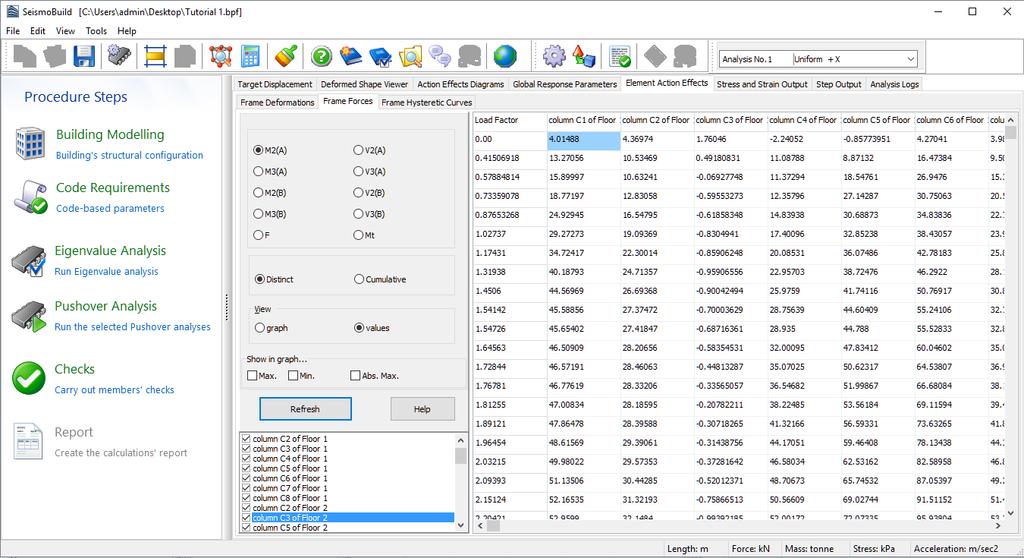
38 38 SeismoBuild User Manual Diagrams for a beam element in 3D Diagrams for a beam element in 2D Show Results Global Response Parameters In the Global Response Parameters module you can output the following results: (i) structural displacements, (ii) forces and moments at the supports, (iii) hysteretic curves and (iv) tables for Codebased Checks. In order to visualise the displacements, in the x direction, of a particular node at the top of the structure, (i) click on the Structural Displacements tab, (ii) select displacement and the x-axis, (iii) select the corresponding node from the list (-> Upper node of column C5 of Floor 2) by ticking the checkbox, (iv) choose the results to visualise (graph or values) and finally (v) click on the Refresh button.

39 Quick Start 39 NOTE: The results are defined in the global system of coordinates and may be exported in an Excel spreadsheet (or similar) as shown below. Global Response Parameters Module (Structural Displacements graph mode) Right click on the values Global Response Parameters Module (Structural Displacements values mode) The total support forces (e.g. total base shear) may be obtained by (i) clicking on the Forces and Moments at Support tab, (ii) selecting force and x-axis and total support forces/moments, (iii) choosing the results to visualise (graph or values) and (iv) clicking on the Refresh button.

40 40 SeismoBuild User Manual Global Response Parameters Module (Forces and Moments at Supports graph mode) Further, the capacity curve of your structure (i.e. total base shear vs. top displacement) can be plotted by (i) clicking on the Hysteretic Curves tab, (ii) selecting displacement and x-axis, (iii) selecting the corresponding node from the drop-down menu (e.g. Control Node), (iv) selecting the Total Base Shear/Moment option, (v) choosing the results to visualise (graph or values) and finally (vi) clicking on the Refresh button. Global Response Parameters Module (Hysteretic Curves graph mode) In order to have the shear forces with a positive sign, (i) right-click on the 3D plot window, (ii) select Post-Processor Settings and (iii) insert the value -1 as Y-axis multiplier.

41 Quick Start 41 Global Response Parameters Module (Hysteretic Curves graph mode) Fourth, in order to visualise the Code-based checks in every step of the analysis of your structure, (i) click on the Code-based Checks tab, (ii) select the chordrot_cap_dl Code-based check, (iii) select to view All (i.e. even the calculations for the members that have not reached their capacity), (iv) select the Output steps that correspond to the Damage Limitation limit state (i.e. Output LS of DL) and finally (vi) click on the Refresh button. Global Response Parameters Module (Code-based Checks) Show Results Element Action Effects In order to proceed with the seismic verifications prescribed in Eurocode 8 it is necessary to check the element chord rotations and element shear forces. For this reason the Frame Deformations and the Frame Forces tab windows may be very useful. The element chord rotations can be directly output by

42 42 SeismoBuild User Manual (i) clicking on the Frame Deformations tab, (ii) selecting chord rotation in the direction you are interested in (i.e. R2), (iii) selecting the elements from the list, by ticking the corresponding box, (iv) choosing the results to visualise (graph or values) and finally (v) clicking on the Refresh button. The element shear forces can be output by (i) clicking on the Frame Forces tab, (ii) selecting shear in the direction and the section you are interested in (i.e. V2(A)), (iii) selecting the elements from the list, by ticking the corresponding box, (iv) choosing the results to visualise (graph or values) and finally (v) clicking on the Refresh button. Element Action Effects Module (Frame Deformations graph mode) Element Action Effects Module (Frame Forces values mode) NOTE: The results may be easily exported in an Excel spreadsheet (or similar).

43 Quick Start 43 Checks SeismoBuild provides the option to automatically undertake chord-rotation and shear checks for structural elements, as well as the necessary beam-column joints checks (shear forces, horizontal hoops area and vertical reinforcement area), according to the expressions defined in the selected Code, and for the selected limit states. This can be visualised in the Checks module of the program's Main Window. The Checks area features a series of pages where the results of the structural members checks can be visualised, in table and graphical format, and then copied into any other Windows application. Users may select the limit state, as well as the analysis, the floor, the type of members and the local axis to view the results. The elements, where the demand has exceeded the capacity, are displayed in red both in the table and the 3D plot, as it is depicted in the figure below: Checks Module (Members Chord Rotations) Report After running the analyses and finishing the checks process, you may create the technical report of the assessment. Once you click on the Report button a window will appear in order to define the print output options. Click the OK button and the report will automatically be created and shown on screen. The report may be exported in PDF, RTF or HTML file formats, the two latter being editable. NOTE: Creating a report for a typical 4 or 5-storey building may take up to 4-5 minute to complete.

44 44 SeismoBuild User Manual Print-out Options (General information) Technical Report

45 Quick Start 45 CAD Drawing Finally, you may export a variety of CAD drawing files of the structural model (plan views, members' cross sections and reinforcement tables), together with specially created *.ctb files that are needed for plotting. It is noted that running the analyses is not a prerequisite for the exportation of the Cad drawing files, and only the introduction of the structural configuration in the Building Modeller is required. Export to DWG

46 46 SeismoBuild User Manual CAD drawing Congratulation, you have finished your first tutorial! TUTORIAL N.2 ASSESSMENT OF A THREE-STOREY BUILDING Problem Description Let us try to model a three dimensional, three-storey reinforced concrete building for which you are asked to assess its capacity according to the Eurocodes. The geometry of all the floors is the same and is shown in the corresponding plan-views below, the only difference being the presence of inclined slabs on the third floor.

47 Quick Start 47 Plan view of the 1 st and 2nd floor of the building NOTE: A movie describing Τutorial N.2 can be found on Seismosoft s YouTube channel. Plan view of the 3 rd floor of the building

48 48 SeismoBuild User Manual Getting started: a new project Section plan The introduction of structural members is the same with the Tutorial N.1, hence, in the current tutorial only the steps for the definition of the stairs and the inclined slabs will be described. For this tutorial the following settings have been chosen: Eurocode 8, Part 3 SI Units European sizes for rebar typology 3 Storeys Storeys heights: 3m Do not accept beams with free span less than: 0.1m Include beam effective widths A CAD drawing is imported as a background to facilitate the definition of the elements geometry.

49 Quick Start 49 Building Modeller CAD drawing insertion In the material sets module the member s concrete and reinforcement strength values are determined. Herein the Default_Existing material set is selected and edited by assigning the C16/20 concrete class and the S400 steel class. Building Modeller Modify Existing Material Scheme By clicking on the Advanced Member Properties button users may define the settings for the structural member according to the selected Code. The selected properties for the inserted members are shown in the figure below:

50 50 SeismoBuild User Manual Building Modeller Advanced Member Properties The dimensions and the reinforcement of the members (columns and beams) of the typical floor are shown in the following tables: Columns Height (mm) Width (mm) Longitudinal reinforcement Transverse reinforcement C /25 C /25 C /25 C /25 C /25 C /25 C /25 C /25 C /25 C /25 C /25

51 Quick Start 51 Columns Height (mm) Width (mm) Longitudinal reinforcement Transverse reinforcement C /25 C /25 C /25 C /25 C /25 C /25 C /25 Beams Height (mm) Width (mm) Reinforcement at the Start of the beam Reinforcement at the Middle of the beam Reinforcement at the End of the beam Transverse reinforcement B o3 16 u2 14 o2 12 u4 14 o3 16 u2 14 8/25 B o3 16 u2 14 o2 12 u4 14 o3 16 u2 14 8/25 B o3 16 u2 14 o2 12 u4 14 o3 16 u2 14 8/25 B o3 16 u2 14 o2 12 u4 14 o3 16 u2 14 8/25 B o3 16 u2 14 o2 12 u4 14 o3 16 u2 14 8/25 B o3 16 u2 14 o2 12 u4 14 o3 16 u2 14 8/25 B o3 16 u2 14 o2 12 u4 14 o3 16 u2 14 8/25 B o3 16 u2 14 o2 12 u4 14 o3 16 u2 14 8/25 B o3 16 u2 14 o2 12 u4 14 o3 16 u2 14 8/25 B o3 16 u2 14 o2 12 u4 14 o3 16 u2 14 8/25 B o3 16 u2 14 o2 12 u4 14 o3 16 u2 14 8/25 B o3 16 u2 14 o2 12 u4 14 o3 16 u2 14 8/25 B o3 16 u2 14 o2 12 u4 14 o3 16 u2 14 8/25 B o3 16 u2 14 o2 12 u4 14 o3 16 u2 14 8/25 B o3 16 u2 14 o2 12 u4 14 o3 16 u2 14 8/25

52 52 SeismoBuild User Manual Beams B16 Height Width (mm) (mm) Reinforcement at the Start of the beam Reinforcement at the Middle of the beam Reinforcement at the End of the beam Transverse reinforcement o3 16 u2 14 o2 12 u4 14 o3 16 u2 14 8/25 After inserting all the columns and beams you may assign the stairs from the main menu (Insert > Insert Stairs) or through the toolbar button. This can be easily done by specifying the centreline and some basic geometric parameters, such us the stairs width, the riser height, the stairs minimum depth, and the elevation differences relatively to the base floor and the top floor, as well as the additional permanent and live loads. Building Modeller Stairs Properties Type of Loaded Area

53 Quick Start 53 After inserting all the members of the 1st floor, you may automatically create the 2nd and 3rd floors based on the already created 1st one by using the Copy Floor facility. Building Modeller Copy Floor dialogue box Delete the elements (e.g. the stairs) that are not present in the 3rd floor and define the inclined slabs. Select the slab that will be modified, click on the Inclined or elevated slab (defined by 3points) checkbox in the slab s properties window, define graphically the coordinates of the 3 points and assign their elevation. Building Modeller Slab Element Properties When you create a building model, it is relatively common that one or more very short beams have been created unintentionally, due to graphical reasons (e.g. by extending slightly a beam s end beyond a column edge). For this reason, a check from the main menu (Tools > Verify Connectivity...) or through the toolbar button for the existence of any beam with free span smaller than its section height should be carried out. If such beams exist, the following message appears, and the user can select to remove or keep the member.

54 54 SeismoBuild User Manual Building Modeller Verify Connectivity With the building model now fully defined, save the project as a SeismoBuild file (with the *.bpf extension, e.g. Tutorial_2.bpf) from the main menu (File >Save As...)/(File >Save) or through the corresponding toolbar button. You are ready to go to the SeismoBuild Main Window. This can be done from the main menu (File > Exit * Create 3D Model) or through the toolbar button. SeismoBuild Main Window Code Requirements The Code-based parameters and options are defined as in Tutorial N.1, apart from the seismic action where: A peak ground acceleration equal to 0.16g is specified; this acceleration is referred to a return period of 475 years, 5% damping, response spectra Type 1, ground type A and Importance class II;

55 Quick Start 55 Analysis & Modelling Parameters The default predefined settings scheme is employed for the scope of this tutorial. Eigenvalue Analysis Run the eigenvalue analysis through this module. Eigenvalue Analysis You may see the results after running the analysis by clicking on the Show Results button.

56 56 SeismoBuild User Manual Eigenvalue Analysis Resuts Pushover Analysis Click on the Run button to run all the selected pushover analyses. Running the analysis When the analyses have arrived to the end, you may see the results by clicking on the Show Results button. The available modules have been discussed in Tutorial N1. Checks The results of the structural members checks can be visualised in the Checks area, in table or graphical format, and then copied into any other Windows application. Users may select the limit state,

57 Quick Start 57 as well as the analysis, the floor, the type of members and the local axis to view the results. The elements, where the demand has exceeded the capacity, are displayed in red both in the table and the 3D plot, as it is depicted in the figure below: Checks Module (Member Shear Forces) Report After running the analyses and finishing the checks process, you may create the technical report of the assessment. Once you click on the Report button a window will appear in order to define the print output options. Click the OK button and the report will automatically be created and shown on screen. The report may be exported in PDF, RTF or HTML file formats, the two latter being editable. NOTE: Creating a report for a typical 4 or 5-storey building may take up to 4-5 minute to complete. Print-out Options (General information)

58 58 SeismoBuild User Manual CAD Drawing Technical Report Finally, you may export a variety of CAD drawing files of the structural model (plan views, members' cross sections and reinforcement tables), together with specially created *.ctb files that are needed for plotting. It is noted that running the analyses is not a prerequisite for the exportation of the Cad drawing files, and only the introduction of the structural configuration in the Building Modeller is required. Export to DWG

59 Quick Start 59 CAD drawing TUTORIAL N.3 REHABILITATION OF A THREE-STOREY BUILDING Problem Description In this third tutorial the model that has already been created in Tutorial N2 will be strengthen with RC jackets. The columns of all the floors will be strengthened, as well as the beams of the first and second floor. Getting started: opening an existing project Open again the initial window of the software and, after clicking on icon on the toolbar, select the previous SeismoBuild project (Tutorial_2.bpf). Once opened, save the project with a new name through File > Save as menu command. In the material sets module the member s concrete and reinforcement strength values are determined. Herein the Default_New material set is selected and edited by assigning the C20/25 concrete class and the S500 steel class.

60 60 SeismoBuild User Manual Building Modeller Modify Existing Material Scheme The dimensions and the reinforcement of the jacketed columns of the first floor are shown in the following table: Columns Height (mm) Width (mm) Internal Longitudinal reinforcement Internal Transverse reinforcement External Longitudinal reinforcement External Transverse reinforcement C / /10 C / /10 C / /10 C / /10 C / /10 C / /10 C / /10 C / /10 C / /10 C / /10 C / /10 C / /10 C / /10

61 Quick Start 61 Columns Height (mm) Width (mm) Internal Longitudinal reinforcement Internal Transverse reinforcement External Longitudinal reinforcement External Transverse reinforcement C / /10 C / /10 C / /10 C / /10 C / /10 The dimensions and the reinforcement of the new/external section of the jacketed beams of the first floor are shown in the following table. It is noted that the reinforcement of the old/internal section of the jacketed beams is the same with that of Tutorial N.2. Beams Height (mm) Width (mm) External Reinforcement at the Start of the beam External Reinforcement at the Middle of the beam External Reinforcement at the End of the beam External Transverse reinforcement B o5 18 u3 14 s4 12 o2 14 s4 12 u5 14 o5 18 u3 14 s /10 B o5 18 u3 14 s4 12 o2 14 s4 12 u5 14 o5 18 u3 14 s /10 B o5 18 u3 14 s4 12 o2 14 s4 12 u5 14 o5 18 u3 14 s /10 B o5 18 u3 14 s4 12 o2 14 s4 12 u5 14 o5 18 u3 14 s /10 B o5 18 u3 14 s4 12 o2 14 s4 12 u5 14 o5 18 u3 14 s /10 B o5 18 u3 14 s4 12 o2 14 s4 12 u5 14 o5 18 u3 14 s /10 B o5 18 u3 14 s4 12 o2 14 s4 12 u5 14 o5 18 u3 14 s /10 B o5 18 u3 14 s4 12 o2 14 s4 12 u5 14 o5 18 u3 14 s /10 B o5 18 u3 14 s4 12 o2 14 s4 12 u5 14 o5 18 u3 14 s /10 B o5 18 u3 14 s4 12 o2 14 s4 12 u5 14 o5 18 u3 14 s /10

62 62 SeismoBuild User Manual Beams Height (mm) Width (mm) External Reinforcement at the Start of the beam External Reinforcement at the Middle of the beam External Reinforcement at the End of the beam External Transverse reinforcement B o5 18 u3 14 s4 12 o2 14 s4 12 u5 14 o5 18 u3 14 s /10 B o5 18 u3 14 s4 12 o2 14 s4 12 u5 14 o5 18 u3 14 s /10 B o5 18 u3 14 s4 12 o2 14 s4 12 u5 14 o5 18 u3 14 s /10 B o5 18 u3 14 s4 12 o2 14 s4 12 u5 14 o5 18 u3 14 s /10 B o5 18 u3 14 s4 12 o2 14 s4 12 u5 14 o5 18 u3 14 s /10 B o5 18 u3 14 s4 12 o2 14 s4 12 u5 14 o5 18 u3 14 s /10 B o5 18 u3 14 s4 12 o2 14 s4 12 u5 14 o5 18 u3 14 s /10 B o5 18 u3 14 s4 12 o2 14 s4 12 u5 14 o5 18 u3 14 s /10 B o5 18 u3 14 s4 12 o2 14 s4 12 u5 14 o5 18 u3 14 s /10 B o5 18 u3 14 s4 12 o2 14 s4 12 u5 14 o5 18 u3 14 s /10 B o5 18 u3 14 s4 12 o2 14 s4 12 u5 14 o5 18 u3 14 s /10 B o5 18 u3 14 s4 12 o2 14 s4 12 u5 14 o5 18 u3 14 s /10 B o5 18 u3 14 s4 12 o2 14 s4 12 u5 14 o5 18 u3 14 s /10 The dimensions and the reinforcement of the jacketed columns of the second and third floors are shown in the following table: Columns 2 nd and 3 rd Floors Height (mm) Width (mm) Internal Longitudinal reinforcement Internal Transverse reinforcement External Longitudinal reinforcement External Transverse reinforcement C / /10

63 Quick Start 63 Columns 2 nd and 3 rd Floors Height (mm) Width (mm) Internal Longitudinal reinforcement Internal Transverse reinforcement External Longitudinal reinforcement External Transverse reinforcement C / /10 C / /10 C / /10 C / /10 C / /10 C / /10 C / /10 C / /10 C / /10 C / /10 C / /10 C / /10 C / /10 C / /10 C / /10 C / /10 C / /10 The dimensions and the reinforcement of the new/external section of the jacketed beams of the second and third floors are the same with those of the first floor. After inserting all the jacketed elements, you check the building model for one or more very short beams that may have been created unintentionally, due to graphical reasons (e.g. by extending slightly a beam s end beyond a column edge) from the main menu (Tools > Verify Connectivity...) or through the respective toolbar button. If such beams exist, the following message appears, and the user can select to remove or keep the element. You are ready to go to the SeismoBuild Main Window. This can be done from the main menu (File > Exit & Create 3D Model) or through the corresponding toolbar button.

64 64 SeismoBuild User Manual SeismoBuild Main Window Code Requirements The Code-based parameters and options are defined as in Tutorial N.2. Analysis & Modelling Parameters The default predefined settings scheme is employed for the scope of this tutorial. Eigenvalue Analysis Run the eigenvalue analysis. Pushover Analysis Click on the Run button to run all the selected pushover analyses.

65 Quick Start 65 Running the analysis When the analyses have arrived to the end, you may see the results by clicking on the Show Results button. The available modules have been discussed in Tutorial N1. Checks SeismoBuild provides the option to automatically undertake chord-rotation and shear checks for structural elements, as well as the beam-column joints checks, according to the expressions defined in the selected Code, herein Eurocode 2 and Eurocode 8, for the selected limit states. The Checks results can be visualised in the Checks module of the default program state, as described in Tutorials 1 and 2. Checks Module (Members Shear Forces)

66 66 SeismoBuild User Manual Report After running the analyses and finishing the checks process, you may create the technical report of the assessment. Once you click on the Report button a window will appear in order to define the print output options. Click the OK button and the report will automatically be created and shown on screen. The report may be exported in PDF, RTF or HTML file formats, the two latter being editable. NOTE: Creating a report for a typical 4 or 5-storey building may take up to 4-5 minute to complete. Print-out Options (General information) Technical Report

67 Quick Start 67 CAD Drawing Finally, you may export a variety of CAD drawing files of the building structural model (plan views, cross sections and reinforcement tables), together with specially created *.ctb files that are needed for plotting. It is noted that running the analyses is not a prerequisite for the exportation of the Cad drawing files. CAD Drawing

68 SeismoBuild Main Menu MAIN MENU AND TOOLBAR SeismoBuild has a simple and easy to understand user interface. The program's Main Window, is subdivided into the following components: Main menu and toolbar: at the top of the program window; 3D Model window: on the centre of the screen Settings bar for the 3D Model: on the right of the program window; Procedure steps list: on the left of the program window. Main Window Area Main menu The main menu is the command menu of the program. It consists of the following sub-menus: File Edit View Tools Help Main toolbar The main toolbar provides quick access to frequently used items from the menu. Main toolbar

69 Quick Start 69 An overview of all the commands necessary to run SeismoBuild is shown below: Command Main menu Shortcut keys Toolbar button New Open Ctrl+N Ctrl+O File Save Ctrl+S Save as - Export Data to SeismoStruct - Export CAD drawings - Edit Copy 3D Plot Ctrl+Alt+C View Model Statistics View Large Icons View Small Icons Analysis & Modelling Parameters 3D Plot Options... - Deformed Shape Settings... - Tools Export to Text File - Create AVI File - Show AVI File... - Calculator - SeismoBuild Help F1 SeismoBuild User Manual SeismoStruct Verification Report SeismoBuild Sample Files Help Seismosoft Forum Video Tutorials Export CAD Drawings Send Message to Seismosoft Seismosoft Website - Register New License - About - A variety of CAD drawing files of the structural model (plan views, cross sections and reinforcement tables) may be quickly created and exported from the main menu (File > Export CAD drawings), together with specially created *.ctb files that are needed for plotting. Users may define the number of exported files (one file per floor) and the information to be included in the CAD file, the units etc.

70 70 SeismoBuild User Manual Export Data to SeismoStruct Export to DWG module The possibility of exporting SeismoStruct projects from the main menu (File > Export Data to SeismoStruct) is available. All the SeismoStruct projects for all the selected analyses (the eigenvalue analysis and all the pushover analyses) will be exported to the folder of the SeismoBuild project. Send Message to Seismosoft Commercial users may send a message to Seismosoft from the main menu (Help > Send Message to Seismosoft) or through the toolbar button. Once the Attach Input File checkbox is selected the model is automatically attached and will be sent to the Seismosoft Support group. It is noted that this facility is available in the Commercial Version only.

71 Send your Message to Seismosoft module Quick Start 71

72 72 SeismoBuild User Manual Analysis & Modelling Parameters All the parameters required for the nonlinear analytical calculations may be defined from the main menu (Tools > Analysis & Modelling Parameters) or from the button. Further information regarding the Analysis & Modelling Parameters may be found in the corresponding chapter of this Manual. 3D PLOT OPTIONS Analysis & Modelling Parameters module The 3D Plot settings of the structural model can be adjusted to best meet the user's preferences and requirements. Display Layout With this facility, accessible through the button on the right, users can (i) select a pre-defined layout, such as Standard Layout (default) and Structural Model (the latter is particularly useful to visualise internal forces results), (ii) save their personal Display Layouts or (iii) change the 3D Plot Options.

73 Quick Start 73 Display Layout Save Current Layout Users may wish to save the changes made in the 3D Plot Options. To do so they have to: Click on the button ; Assign a name to the new layout configuration; Click the OK button to confirm the operation. The new layout will appear in the corresponding drop-down menu. Further, users may always return to the initial default layout by selecting the Standard Layout option from the drop-down list. 3D Plot Options The full range of plotting adjustment parameters, on the other hand, can be found in the 3D Plot Options dialog box, accessible from the main menu (Tools > 3D Plot Options ) or through the button. Within the 3D Plot Options menu, there are a number of submenus from which users can, not only select which model components (nodes, structural members, etc.) to show in the plot, but also change a myriad of settings such as the colour/transparency of elements, the plot axes and background panels, the colour and size of text descriptors, and so on.

74 74 SeismoBuild User Manual 3D Plot Options menu By default, the 3D Plot is automatically updated. In cases where the structural model is very large (several hundreds of elements) and/or the user is using a laptop running on batteries with a sloweddown CPU (so as to increase the duration of battery), the program takes some seconds to update the view. Hence, it might prove to be more convenient for users to disable this feature (uncheck the Automatic 3D Plot Update option in the 3D Plot Options General submenu) and thus opt for manual updating instead, carried out with the Update 3D Plot command found in the 3D Plot Options on the right of the screen. Basic Display Settings These are a list of settings accessible through the button on the right, users can tweak the most commonly used plotting features (view type, rendering options, names show, members axes representation, element transparency, and so on) using the available check-boxes and drop-down menus. Basic Display Settings

75 Quick Start 75 Cut Planes In addition to the previous features, also the Cut Planes option can be activated through the on the right. button Cut Planes Additional operations Users can also quickly zoom, rotate, and move the 3D/2D plot of the structural model, by using either the mouse (highly recommended) or keyboard shortcuts. Further, it is also possible to point&click elements to quickly go to the Building Modeller to view/modify element s properties, or right-click and select "Member Configuration...".

76 Building Modeller A special CAD-based facility is introduced to facilitate the creation of building models. Currently, only reinforced concrete buildings can be created; in subsequent releases of the program steel and composite models will be also supported. The Building Modeller is accessed from the program Main Window by clicking on the Building Modelling button. MODELLING SETTINGS Users are able to define the geometry of the new building and the main settings of the model in the Initialize Building Modelling dialog box. Structural Configuration In the Structural Configuration tab the number of storeys and their heights are defined; a number from 1 to 100 storeys, with different heights at each storey and the possibility of applying a common height to a range of storeys, may be selected. Up to three underground floors (basement storeys) and their heights may also be defined. The default selection for this module is 3 storeys with 3.00m height each without basement storeys. Modelling Settings Structural Configuration

77 Building Modeller 77 Structural Modelling The option of not accepting beams shorter than a specific length is available through the Structural Modelling tab to avoid the creation of very short beams, by mistake (e.g. by extending slightly a beam s edge after the column at its end). The default value for this option is 0.1m. Users may also decide whether to include the effective slab width in the beams modelling. Finally, the definition of the control node is made within this module. Users may select directly the floor of the control node, or alternatively choose the automatic definition, in which the control node is defined at the center of mass of the upper floor or at the floor lower to that (in the case of having a top floor mass less than 10% of the lower floor s), depending on the choice made in the Advanced Settings> Advanced Building Properties. Modelling Settings Structural Modelling It is noted that the Building Modeller settings can be changed later through the toolbar button.

78 78 SeismoBuild User Manual BUILDING MODELLER MAIN WINDOW After defining the building s main settings, the Building Modeller Main Window appears, as shown in the figure below. Building Modeller Main Window INSERTING A BACKGROUND The possibility of inserting as background a CAD drawing is offered from the main menu (File > Import DWG...) or through the corresponding toolbar button. Once the drawing is inserted the user is asked to specify drawing s units and to choose whether to move the DWG/DXF file to (0,0), i.e. to the origin of the coordinates system. Selecting this checkbox moves the bottom-left edge of the drawing to the (0,0) coordinates, irrespective of its initial CAD coordinates. Imported Cad Settings window Note that the axes origin can be further moved to a different point that might be more suitable after loading the CAD file with the Move Axes Center ( ) toolbar button, also accessible from the main menu (View > Move Axes Center). The option of moving the imported CAD file is also available through the Move DWG ( ) toolbar button or from the main menu (View > Move DWG). Further, from the main

79 Building Modeller 79 menu (View > Show/Hide DWG) or through the toolbar button is defined whether the CAD drawing will be visible or not. Users may also move the building in plan view from the main menu (Tools > Move Building) or from the corresponding toolbar button by either assigning the relative coordinates or by selecting the base point and the second point graphically. Move Building window The option of rotating the building in plan view is also available from the main menu (Tools > Rotate Building) or from the toolbar button. Users should specify the base point by its coordinates or graphically and assign the rotation angle. Rotate Building window Finally, the layout of an existing floor may be used as background in order to easily introduce new members on another storey.

80 80 SeismoBuild User Manual New Floor & Background INSERTING STRUCTURAL MEMBERS The Material Sets, the Advanced Member Properties and the Modelling Parameters are common to all the sections properties windows while FRP Wrapping is available only for columns. Note that a HowTo documents list is introduced for a quick access to all the required information regarding modelling within the Building Modeller. Material Sets The material sets properties can be defined from the main menu (Tools > Define Material Sets), through the corresponding toolbar button, or through the Define Material Sets button within the member s properties window. The required values for the definition of the materials properties depend on the type of the members, i.e. existing or new members. For existing materials the mean strength value and the mean strength value minus the standard deviation are required, whereas for new materials the characteristic strength value and the mean strength value should be assigned. By default, there are two material schemes, one for the existing elements and one for the new ones. Users may modify the values of the default sets, but they can also add new material sets to cover the needs of their model (e.g. when different material strengths are employed). Material Sets Window

81 Building Modeller 81 Add New Material Scheme NOTE 1: There is a limit to the number of the defined material schemes equal to 10. The default material sets cannot be removed. NOTE 2: The option of applying predefined material strengths, depending on the year of construction of the building, is available when this is allowed from the selected Code. Advanced Member Properties The member s code-based settings may be defined from the Advanced Member Properties dialog box accessed by the Properties Window. Herein, users may determine the element s classification (i.e. primary or secondary seismic member), whether it is with or without detailing for earthquake resistance, its cover thickness, the type of the longitudinal bars (cold-worked brittle steel and smooth (plain) longitudinal bars may be assigned), the type and length of lapping for the longitudinal bars, as well as the accessibility of area of intervention (needed for the Greek Seismic interventions Code only). It is noted that the length of lapping may be defined in three ways; (i) the members have adequate relative lap length, compared with the minimum lap length for ultimate deformation (default option); (ii) the members have inadequate relative lap length (the ratio between the applied lap length and the minimum lap length for ultimate deformation should be defined); and (iii) the members have inadequate lap length (the absolute lap length should be assigned).

82 82 SeismoBuild User Manual Modelling Parameters Advanced Member Properties module The member s modelling parameters may be defined from the Modelling Parameters dialog box, accessed by the Properties Window. Herein, users may define the concrete and steel material types and the frame element type that will be used to model the structural member in SeismoBuild, together with other modelling options, such as the number of sections fibres and the assignment of Moment/Force releases. Materials and frame element types that are to be used within a SeismoBuild project come defined in the Advanced Building Modelling tab of the Advanced Settings module. The choices made in the Advanced Building Modelling tab are the Default options within the Member Modelling Parameters tab. Eleven material types are available in SeismoBuild, four types for concrete and seven for steel. The complete list of materials is proposed hereafter: Mander et al. nonlinear concrete model - con_ma Trilinear concrete model - con_tl Chang-Mander nonlinear concrete model con_cm Kappos and Konstantinidis nonlinear concrete model - con_hs Menegotto-Pinto steel model - stl_mp Giuffre-Menegotto-Pinto steel model - stl_gmp Bilinear steel model - stl_bl Bilinear steel model with isotropic strain hardening- stl_bl2 Ramberg-Osgood steel model - stl_ro Dodd-Restrepo steel model stl_dr Monti-Nuti steel model - stl_mn For a comprehensive description of the material types, refer to Appendix C Materials. Different frame element types may be employed within the structural members. Users may select between inelastic force-based frame elements (infrmfb), inelastic plastic-hinge force-based frame

83 Building Modeller 83 elements (infrmfbph), inelastic plastic-hinge displacement-based frame elements (infrmdbph), inelastic displacement-based frame elements (infrmdb) and elastic frame elements (elfrm). The inelastic displacement-based frame element type (infrmdb) is suggested to be employed for short members, a choice that improves both the accuracy and the stability of the analysis. NOTE: Code based checks are not executed for the member of the elastic frame element type (elfrm). Hence, this element type may be employed only for special modelling cases, when an elastic member behaviours is expected. Further, the number of section fibres used in equilibrium computations carried out at each of the element's integration sections needs to be defined. User may assign the number of fibres of their choice or they may select the automatic calculation, according to which 50 fibres are defined for a member s concrete area less than 0.1m 2 and 200 fibres for a member s concrete area more than 1m2, whereas linear interpolation is executed for the in between values. Each longitudinal reinforcement bar is defined with 1 additional fibre; added to the abovementioned concrete number of fibres. Finally, users may also 'release' one or more of the element degrees of freedom (forces or moments). FRP Wrapping Modelling Parameters module FRP wraps may be assigned to columns through the FRP Wrapping module. Users may select the FRP sheet from a list of the most common products found in the market, or alternatively introduce userdefined values. The number of applied layers may also be defined, as well as whether the dry or the laminate FRP properties are to be used in the calculations. Finally, for the rectangular cross sections the radius of rounding of the corners R may be specified, a critical parameter in the application of FRP wraps.

84 84 SeismoBuild User Manual Select from a list module When users choose to specify user-defined values, the required information is the type of the FRP sheet (Carbon, Aramid, Glass, Basalt or Steel fibres), its laminate or dry properties, the number of direction(s) and the orientation (relatively to the longitudinal direction of the sheet) of the fibres, as well as the number of layers and the radius of rounding corners R. User-defined Values module

85 Building Modeller 85 Finally, FRP systems may be proposed to Seismosoft through the Propose FRP system to Seismosoft button. Herein, the user is asked to assign the name of the FRP system, the link where information about the product may be found and the technical properties of the FRP sheet. Column Members Propose FRP System window The columns can be inserted from the main menu (Insert >...) or through the corresponding toolbar buttons. The column's Properties Window will appear where the properties below can be explicitly defined: (i) the dimensions (height, width and if it is full length or free length, assigning the length difference in the last case) (ii) the foundation level (iii) the reinforcement (iv) the material sets (v) the FRP wrapping (vi) the advanced member properties (vii) the modelling parameters The column members may be inserted in the project with a single mouse click. Once the Insert a Column command is selected, an informative message appears providing brief information of how to insert a column.

86 86 SeismoBuild User Manual How-To Insert a Column window Currently, eight section types are available in SeismoBuild: Rectangular Column L-Shaped Column T-Shaped Column Circular Column Rectangular Jacketed Column L-Shaped Jacketed Column T-Shaped Jacketed Column Circular Jacketed Column For a comprehensive description about the insertions of columns in the Building Modeller refer to Appendix D - Inserting Structural Members.

87 Building Modeller 87 Wall Members The walls can be inserted from the main menu (Insert >...) or through the corresponding toolbar button. The wall's Properties Window will appear where its properties are explicitly defined in the similar way to the columns. The walls may be inserted in the project by defining their edges; only two mouse clicks are needed. Currently, the following types are available in SeismoBuild: Wall Compound Wall Once the Insert a Wall command is selected, an informative message appears providing brief information of how to insert a wall. How-To Insert a Wall window For a comprehensive description about the insertions of walls in the Building Modeller refer to Appendix D - Inserting Structural Members. If the Insert Compound Wall toolbar button is selected, an informative window will appear proposing the best way to insert compound wall sections. According to recent research, (Beyer K., Dazio A., and Priestley M.J.N. [2008]), the best way to subdivide non-planar wall systems, e.g. U-shaped or Z-shaped walls, into planar subsections is by splitting the corner area between the flange and the wall elements. In this way the inner corner bar is attributed to both the web and the flange section, while the outer bar is not assigned to any section, the total reinforcement area is therefore modelled correctly.

88 88 SeismoBuild User Manual Modelling of Wall Systems message NOTE: Horizontal links are automatically assigned by the program in order to connect the defined vertical elements. Beam Members The beams can be inserted from the main menu (Insert > ) or through the corresponding toolbar buttons. Several additional parameters, in addition to those provided for columns, need to be specified for the correct definition of a beam, i.e. whether it is an inclined beam (in this case the height of the two ends should be specified), the additional permanent load and the reinforcement in three integration sections of the beam (in the middle and two edges). Beams may be inserted in the project by defining their edges with two mouse clicks. After assigning the beams and the slabs, the choice of including the effective width and customizing its value, as well as if the beam members will be inversed beams, may be made. Currently, two types are available in SeismoBuild: Beam Jacketed Beam Once the Insert Beam command is selected, an informative message appears providing brief information of how to insert a beam.

89 Building Modeller 89 How-To Insert a Beam window For a comprehensive description about the insertions of beams in the Building Modeller refer to Appendix D - Inserting Structural Members.

90 90 SeismoBuild User Manual Slabs The insertion of slabs can be done through the Menu (Insert > Insert Slab) or by clicking the toolbar button. Prior to adding a slab, an informative message appears providing brief information of how to insert a slab. How-To Insert a Slab window A slab can be defined with a single mouse click on any closed area surrounded by structural members (columns, walls and beams). In the slab s Properties Window users can define (i) the section s height, (ii) the reinforcement and its rotation to the X & Y axes, and (iii) its self weight and the additional permanent, live and snow loads; the latter is required only by ASCE and TBDY. The self-weight of the slabs may be automatically calculated and included in the structural model or a user-defined value may be used. The slab's live loads are automatically assigned by the program after the user selects the appropriate type of loaded area.

91 Building Modeller 91 Slab's Properties Window Type of Loaded Area

92 92 SeismoBuild User Manual Slab insertion After defining a slab, users may modify its support conditions, thus adjusting at which beams the slab loads are to be distributed. Slab Support Conditions Further the inclination of the slab may be modified, by specifying the slab elevation at three points that can be graphically selected. The neighbouring beams elevation and column heights are automatically adjusted, whereas the columns are subdivided in shorter members by the program, if this is required, i.e. in the cases where two or more beams are supported by the same column at different levels, thus creating short columns. Slab Inclination

93 Building Modeller 93 NOTE 1: The slab modelling is carried out with rigid diaphragms; hence, a rigid slab is implicitly considered in the structural configuration, which is the case for the vast majority of RC buildings. The slab s loads (self weight, additional gravity and live loads multiplied by the corresponding coefficients in the Static Actions module) are transformed to masses, based on the g value, and applied directly to the beams that support the slab. NOTE 2: The slab reinforcement is applied at the effective width of the beams at the perimeter of the slab. Obviously, when users select not to include the effective width in the modelling, such reinforcement settings become redundant. Slab by perimeter Slabs of any geometry can be defined in the Building Modeller by selecting the Insert > Insert Slab by perimeter from the Menu (or through the respective toolbar button ). An informative message appears providing brief information of how to insert a Slab by perimeter. How-To Insert Slab by its Perimeter After defining the Slab s perimeter by identifying its corners, the Apply & Insert Slab button should be clicked. The slab is automatically assigned. Draw Slab by perimeter

94 94 SeismoBuild User Manual NOTE 1: Slabs are modelled in SeismoBuild as rigid diaphragms that connect the beams, columns and walls in their perimeter and as additional loads applied to the beams. Obviously, in the case of cantilevered slabs no rigid diaphragm is created and a slab is only considered as additional mass on the supporting beam; the additional mass account for the slabs' permanent and live loads. NOTE 2: When the assigned perimeter does not define a closed area, the first point is automatically connected by the program with the last one in order to assign the new slab. Free Edge Cantilever slabs can also be defined in the Building Modeller. In order to do so, a Free Edge must be added from the Menu (Insert > Insert Free edge) or through the respective toolbar button. An informative message appears providing brief information of how to insert a Free Edge. How-To Insert Slab Edges window After defining the Free Edge's corner points, the Apply button should be clicked. Once drawn, the Free Edge is used to outline the shape of the slab. Draw Free Edge

95 Building Modeller 95 After the definition of the necessary free edges needed to define a closed area, users can insert a new slab. Create a new cantilevered slab NOTE: Slabs are modelled in SeismoBuild as rigid diaphragms that connect the beams, columns and walls in their perimeter and as additional loads applied to the beams. Obviously, in the case of cantilevered slabs no rigid diaphragm is created and a slab is only considered as additional mass on the supporting beam; the additional mass account for the slabs' permanent and live loads. Stairs The insertion of stairs can be done through the Menu (Insert > Stairs) or by clicking the button. An informative message appears providing brief information of how to insert Stairs. toolbar How-To Insert Stairs window Stairs may be easily defined by specifying their centreline. Landings may be applied through the Add Landings button after the insertion of the stairs member in the project. The two ends of the landings need to be specified graphically on the centreline. The defined landings may be removed through the Remove All Landings button.

96 96 SeismoBuild User Manual On the Properties Window users can further define the stairs width, the riser height, the stairs minimum depth, the elevation difference relatively to the base and the top floor level, as well as the self-weight and the additional permanent, live and snow loads; the latter is required only by ASCE and TBDY. The self-weight of the stairs may be automatically calculated according to the stairs geometry, materials and specific weight or a user-defined value may be used. Stairs Properties Window Type of Loaded Area NOTE: Slabs are modelled in SeismoBuild with elastic elements of the specified width and depth.

97 Building Modeller 97 EDITING STRUCTURAL MEMBERS By using the edit tools from the main menu (Tools >...) or through the respective toolbar buttons, users can select ( ) a member to view or change its properties. Further they can move it ( ) to a different location, rotate it ( ) in plan view or delete it ( ). It is noted that there is a number of ways to delete elements: (i) by clicking on the element (ii) by its name or (iii) by selecting a rectangular area on the Main Window. Delete element window The option of multi-editing structural members is available from the main menu (Tools > View/Modify Member Properties) or through the corresponding toolbar button. Users may select multiple members of the same section type and modify their properties at once. View/Modify Member Properties window The properties of one member may be applied to others from the main menu (Tools > Copy Member Properties) or through the corresponding toolbar button. A window with a list of the properties that will be copied appears after the selection of the member. Users should just click on a member in order to change its properties. It is noted that the additional rebars cannot be copied.

98 98 SeismoBuild User Manual Copy Member Properties window Moreover, an option to renumber the structural members is offered from the main menu (Tools > Renumber Elements) or through the toolbar button. By clicking on a member the selected number is assigned to it, and the numbering of all other members is changed accordingly. After creating a building model, it is relatively common that one or more very short beams have been created unintentionally, due to graphical reasons (e.g. by extending slightly a beam s end beyond a column edge). For this reason, a check is carried out from the main menu (Tools > Verify Connectivity...) or through the corresponding toolbar button for the existence of any beam with free span smaller than its section height should be carried out. If such beams exist, the following message appears, and the user can select to remove or to keep it. CREATING NEW STOREYS Verify connectivity The possibility of automatically creating new floors, based on the already created ones is offered through the main menu (Tools > Copy Floor...) or through the toolbar button. Copy floor

99 Building Modeller 99 It is noted that users may use the layout of an existing floor as background, in order to easily introduce new members on another storey. New Floor & Background

100 100 SeismoBuild User Manual VIEW STOREY 3D MODEL The possibility of viewing the 3D model of the current floor is offered through the main menu (View > Storey 3D Model...) or through the toolbar button. OTHER BUILDING MODELLER FUNCTIONS 3D View of Storey window The Building Modeller offers a variety of tools to facilitate the introduction of the structural layout: Different zoom tools are available to users (zoom in, zoom out, dynamic zoom, zoom to window, center all and zoom to member). These tools are also available through the respective toolbar buttons or through the main menu (View >...). Zoom tools Showing or hiding the CAD drawing as a background image can be done from the main menu (View > Show/Hide DWG...) or through the corresponding toolbar button, after it has been loaded with the button. Snap tools offer the possibility of snapping to the CAD drawing, the element and/or the grid. The grid properties (step, min and max values) and the snap properties (step), as well as whether the grid will be visualised or not may be defined from the Snap and Grid Properties dialog box accessed by the main menu (View > Snap & Grid Properties) or through the toolbar button.

101 Building Modeller 101 Snap & Grid Properties Further, an Ortho facility is provided; Ortho is short for orthogonal, and allows for the introduction of either vertical or horizontal - but not inclined - line (beams or walls) members. Again, all these facilities can be accessed from both the main menu (View >...) and through the corresponding toolbar buttons. Snap and Ortho tools The axes origin of the CAD drawing at the background can also be moved from the main menu (View >Move Axes Centre) or through the toolbar button. Move Axes Center The building in plan view may also be moved from the main menu (Tools > Move Building) or through the toolbar button. The option of rotating the building in plan view is available from the main menu (Tools > Rotate Building) or from the toolbar button. The possibility of undoing and redoing the last operations is offered (Edit >Undo)/ (Edit >Redo) or through the buttons. The selected plan view can be printed or previewed from the main menu (File >Print... & File >Print Preview...) or through the respective toolbar buttons &

102 102 SeismoBuild User Manual Print Preview SAVING AND LOADING SEISMOBUILD PROJECTS The SeismoBuild project (with the *.bpf extension) may be saved from the main menu (File >Save As...)/(File >Save) or through the toolbar button. These files can be opened again from the Main Window of SeismoBuild (File >Open) or through the corresponding toolbar button. The 3D SeismoBuild model may be visualised by selecting the & Create 3D Model). button or the main menu (File >Exit New SeismoBuild model

103 Building Modeller 103 NOTE: When creating a SeismoBuild project file from the Building Modeller, the structural mass is modelled by the material's specific weight, and the sections' additional mass parameters. The former accounts for the mass of the columns, the walls and the beams, while the latter accounts for the mass that corresponds to the slabs' self weight, additional permanent loads and live loads. These defined masses are transformed to gravity loads, based on the g value.

104 Structural Modelling After the model input is defined in the Building Modeller the program automatically creates the structural model according to the following rules: The structural members are modelled with fibre-based inelastic frame elements. Both geometric nonlinearities and material inelasticity are considered. Furthermore, the offsets at the beam-column joints are automatically calculated and included in the structural model. Eleven nonlinear material models are available for modelling the concrete and steel behaviour. The Mander et al. [1988] model and the Menegotto-Pinto [1973] model are employed by default for concrete and steel, respectively. A specially created model for high strength concrete is also available. Five element types are available, consisting of a combination of force-based and displacement based inelastic elements, with distributed plasticity or lumped plasticity (plastic-hinge elements), as well one elastic element type. In particular the available element types are: (i) Inelastic force-based frame element type - infrmfb, (ii) Inelastic force-based plastic hinge frame element type- infrmfbph, (iii) Inelastic displacement-based plastic hinge frame element type - infrmdbph, (iv) Inelastic displacement-based frame element type - infrmdb, and (v) Elastic frame element type elfrm. The inelastic displacement-based frame element type is generally used for members of small length, e.g. to model short columns. With the distributed plasticity formulations (infrmfb and infrmdb), the spread of inelasticity along the member length and across the section depth is explicitly modelled, allowing for the accurate estimation of damage accumulation. This is of particular importance in the modelling of walls at the lower floors and especially at the ground level, where the large bending moments and the distribution of plasticity are not concentrated at the member ends (in which case a plastic-hinge approach would be adequate), but rather along the entire storey height. Considering the dominant role that large shear walls play in the overall structural behaviour, this feature sets apart SeismoBuild from other similar assessment packages that model all the structural members with plastic-hinge element, and thus do not simulate the distribution of inelasticity along the entire height of the ground floor. The default element types employed are the lumped plasticity (plastic-hinge) force-based elements infrmfbph for the columns and beams, and the distributed plasticity force-based elements infrmfb for the walls. For short elements the distributed plasticity displacementbased is employed, for reasons of improved analysis stability and better convergence. Specifically for the beams, different cross section are considered in the elements integration sections, according to the specified reinforcement patterns (longitudinal and transverse) at the start, middle and end of the member. In the columns and the walls one cross-section is employed throughout the length of the member. The diaphragmatic action of the slabs is modelled though rigid diaphragms. The stairs are modelled with elastic elements of the specified width and depth. The column and beam masses are directly included in the model. The slab masses are applied to the supporting beams as additional masses and loads. The default option for the location of the control node is automatically determined by the program as the centre of mass of the upper floor or of the floor lower to that (in the case of having a top floor mass less than 10% of the lower floor s). Users may define the control node at a different floor. The column elements are considered fixed at the foundation level. Different foundation levels and at different floors may be employed for different columns of the same structure.

105 Building Modeller 105 SeismoBuild Main Window Show FE Model Member offsets

106 Code Requirements The Code requirements may be defined through a dialog box accessed by SeismoBuild window. in the main The Code Requirements area features a series of pages where the necessary settings for the analyses and the checks may be determined according to the selected Code or Standard. The available Codes in the current version of SeismoBuild are the Eurocode 8- Part 3, the American Code for Seismic Evaluation and Retrofit of Existing Buildings (ASCE 41-13), the Italian National Seismic Code (NTC-18), the Italian National Seismic Code (NTC-08), the Greek Seismic Interventions Code (KANEPE) and the Turkish Seismic Evaluation Building Code (TBDY); once the Code is selected the pages are respectively modified. Available Codes The available pages within the Code Requirements area are listed below and will be described in detail in the following paragraphs: Limit States (Performance Objectives in KANEPE) Analysis Type Knowledge Level Seismic Action Static Actions Interstorey Drift Limits (Only in NTC) Target Displacement (Only in KANEPE) Checks NOTE: The available Codes depend on the edition of the SeismoBuild. Users should select the edition with the required Codes. LIMIT STATES Herein users may define the Limit States or the Performance Levels to be used to check the structure. In the cases of the Eurocodes, the state of damage in the structure is defined through three limit states, namely Near Collapse (NC), Significant Damage (SD) and Damage Limitation (DL). It is noted that the

107 Code Requirements 107 selection of the limit state(s) that need to be checked in a country may be found in the relevant National Annex. The performance levels employed in ASCE consist of combinations of the target building performance levels (Operational Level, Immediate Occupancy, Life Safety and Collapse Prevention) and seismic actions (2%, 5%, 20% and 50% probabilities of exceedance of the seismic action within a conventional life cycle of 50 years). The corresponding limit states for the Italian Code are four, i.e. limit state of Operational Level (OL), Damage Limitation (DL), Life Safety (LS) and Collapse Prevention (CP). Apart from the considered limit states, users may specify the location of the structure in the Italian territory, the life time of the structure and its importance class, and the parameters needed for the spectra derivation are automatically calculated. The performance objectives employed in KANEPE consist of combinations of the performance requirements (Immediate Occupancy, Life Safety and Collapse Prevention) and seismic actions (10% and 50% probabilities of exceedance of the seismic action within a conventional life cycle of 50 years). The performance levels for the TBDY consist of combinations of the target building performance levels (Continuous Use, Immediate Occupancy, Life Safety and Collapse Prevention) and seismic actions (2%, 10%, 50% and 68% probabilities of exceedance of the seismic action within a conventional life cycle of 50 years). A detailed description on the limit states is available in the corresponding appendix for the selected Code (Appendix A.1 EUROCODES, Appendix A.2 ASCE, Appendix A.3 NTC-18, Appendix A.4 NTC- 08, Appendix A.5 KANEPE, Appendix A.6 - TBDY). ANALYSIS TYPE Limit States module In SeismoBuild the most common method in assessment practice of existing buildings is employed, which is the nonlinear static analysis. It is based on pushover analyses carried out under constant gravity loads and increasing lateral forces, applied at the location of the masses to simulate the inertia forces induced by the seismic action. As the model may account for both geometrical and mechanical nonlinearity, this method can describe the evolution of the expected plastic mechanisms and structural damage. The different load patterns that will be applied to the structure are defined in this module in two ways:

108 108 SeismoBuild User Manual The first one is by selecting one of the pattern schemes as defined by the Codes, i.e. (i) Basic Combinations, (ii) Eurocode 8, (iii) ASCE 41-13, (iv) NTC-08, (v) NTC-18 (vi) KANEPE and (vii) TBDY. By choosing one of these schemes the appropriate load patterns will be selected. The second way is to choose individual user-defined load patterns from the corresponding checkboxes. Users may decide about the vertical distribution of loads (uniform and/or modal patterns), the simultaneous or not application of the lateral incremental loads in the two horizontal directions (Uniaxial or Biaxial load patterns) and the existence or not of Single and/or Double Eccentricity. Analysis Type module Users may refer to the General section of Pushover Analysis of this Manual for further information about the loading patterns. KNOWLEDGE LEVEL In this module users may select the Knowledge Level that corresponds to the available data on the structural configuration. Three knowledge levels are defined. A more detailed description on the factors determining the achieved knowledge level is available in Appendix A.1 EUROCODES, Appendix A.2 ASCE, Appendix A.3 NTC-18, Appendix A.4 NTC-08, Appendix A.5 KANEPE, Appendix A.6 TBDY. The default values for the confidence factor are those recommended in the corresponding Code, although it is also possible to assign different values by selecting the Custom value checkbox (e.g. according to the country s National Annex for the case of Eurocodes).

109 Code Requirements 109 Knowledge Level module SEISMIC ACTION Herein the elastic response spectrum (as specified in the selected Code) is determined, and scaled to the values of the design ground acceleration established for the different Limit States. Users should assign the basic parameters needed for the generation of the spectral shape (i.e. peak ground acceleration, damping, spectrum type, ground type and important class). For further information you may refer to the corresponding section of the selected Code (Appendix A.1 EUROCODES, Appendix A.2 ASCE, Appendix A.3 NTC-18, Appendix A.4 NTC-08, Appendix A.5 KANEPE, Appendix A.6 TBDY). Seismic Action module

110 110 SeismoBuild User Manual STATIC ACTIONS The permanent and live loads coefficients are assigned in this module. As described in the General section of Pushover Analysis, in addition to the introduced vertical loads in nonlinear static analyses the permanent and live loads are applied, which are also used for the definition of the structural mass in the Eigenvalue Analysis. The snow load coefficient is also assigned in the case of ASCE or TBDY. Static Actions module INTERSTOREY DRIFT LIMITS In NTC an additional check may be executed for the limit states of Operational Level and Damage Limitation, as described in the Interstorey Drifts section of Appendix A.3 NTC-18 and Appendix A.4- NTC-08. Users may define through this module whether the infills will be considered as rigidly connected to the structure, or are expected to suffer no damage, in order to specify the target relative deformation at each floor. Alternatively, they can assign user-defined values, by selecting the other modelling option.

111 Code Requirements 111 Interstorey Drift Limits module TARGET DISPLACEMENT Herein the structural type of the building is specified for the proper definition of the C2 factor, taken into consideration in the Target Displacement calculations of KANEPE (see the Target Displacement section of Appendix A.5 KANEPE CHECKS Herein, the checks to be carried out according to the selected Code for structural members and beamcolumn joints may be selected. The available checks within all the employed Codes are the following: Members Chord Rotations Members Shear Forces Members Strains (Only for TBDY) Joints Shear Forces (Eurocode 8, ASCE & TBDY) Joints Horizontal Hoops Area (Only for Eurocode 8) Joints Vertical Reinforcement Area (Only for Eurocode 8) Joints Diagonal Tension (NTC & KANEPE) Joints Diagonal Compression (NTC & KANEPE) Interstorey Drifts (ASCE & NTC) A more detailed description on the checks and the equations used in SeismoBuild is available in the Checks and in the Capacity Models for Assessment and Checks of Appendix A.1 EUROCODES, Appendix A.2 ASCE, Appendix A.3 NTC-18, Appendix A.4 NTC-08, Appendix A.5 KANEPE, Appendix A.6 TBDY, respectively.

112 112 SeismoBuild User Manual Checks module The values of the safety factors used in the checks may be specified through the corresponding button, as well as the employed Code expressions. The program default factors are those defined in the selected Code. Safety Factors module

113 Analysis & Modelling Parameters Users are able to define all the parameters required for the nonlinear analytical calculations within this module, by selecting a predefined settings scheme, by clicking on the Advanced Settings button or double-clicking on a specific value to open the corresponding tab in the Advanced Settings module. SETTINGS SCHEMES Because of the requirement for advanced and specialised knowledge for most of the analysis parameters (e.g. material models, frame element type, convergence criteria tolerances, rigid diaphragm modelling), ten predefined schemes are available that define the more important analysis parameter settings. Settings Schemes bar These predefined Settings Schemes have been chosen so as to fit the requirements of multiple types of analysis and models, leading to optimised solutions in terms of performance efficiency and results accuracy. Depending on a model s particular characteristics and demands, different Settings Schemes might fit at different cases; the program carries out an internal check and a notification message is issued, whenever one or more of the settings do not seem to suit the needs of the specific project. The notification messages that might appear are the following: The selected settings scheme seems reasonable, which means that with the selected combination users will probably not face convergence difficulties or accuracy problems during the analyses; Strict convergence criteria. Convergence problems might arise; the program warns for possible convergence problems that might arise because of the strict convergence criteria chosen; Very strict convergence criteria. Convergence problems will probably arise; the program warns for possible convergence problems that will probably arise because of the very strict convergence criteria chosen; Loose convergence criteria. Accuracy problems might arise; the program warns for possible accuracy problems that might arise because of the loose convergence criteria chosen; Very loose convergence criteria. Accuracy problems will probably arise; the program warns for possible accuracy problems that will probably arise because of the very loose convergence criteria chosen. When a chosen settings scheme does not seem reasonable, a See Why button appears on the right side of the bar. By clicking on this button users are able to see why the selected settings scheme should not be applied to their model, and which specific settings need to be changed to improve them.

114 114 SeismoBuild User Manual See Why window ADVANCED SETTINGS For each SeismoBuild project it is possible to customise both the usability of the program as well as the performance characteristics of analytical proceedings, so as to better suit the needs of any given structural model and/or the preferences of a particular user. This program/project facility is available from the Analysis Parameters module or the Advanced Settings panel, which can be accessed through the Advanced Settings button. The Advanced Settings panel features a number of tab windows, which provide access to different type of settings, as described below: General Analysis Elements Constraints Convergence Criteria Iterative Strategy Gravity & Mass Eigenvalue Advanced Building Modelling Cracked Stiffness Analysis settings tab windows Common to all tab windows are the Program Defaults and Set As Default options found at the bottom of the Advanced Settings panel. The Set As Default option is employed whenever the user wishes to define new personalised default settings, which will then be used in all new projects subsequently created. The Program Defaults, on the other hand, can be used to reload, at any time,

115 Analysis Parameters 115 the original program defaults, as defined at installation time. Note, however, that the Program Defaults option does not change the default program settings; it simply loads the installation settings in the current project. Hence, if the user has previously personalised the default settings of the program (using the Set As Default option) and then wishes to revert the program default settings back to the original installation defaults, he/she should first load the Program Defaults and then choose the Set As Default option. Program Defaults and Set as Default options NOTE: For the majority of applications, there is no need for the Advanced Settings default values to be modified, since the available Settings Schemes have been chosen so as to fit the requirements of any building model, leading to optimised solutions in terms of performance efficiency and results accuracy. General The General settings provide the possibility of customising the usability of the program to the user's preferences. Text Output When activated, the Text Output option will lead to the creation, at the end of every analysis, of a text file (*.out) containing the output of the entire analysis (as given in the Step Output module). This feature may result useful for users who wish to systematically post-process the results using their own custom-made post-processing facility. For occasional access to text output, users are instead advised to use the facilities made available in the Step Output module. Multiple Text Output When activated, the Multiple Text Output option will lead to the creation of multiple text files (*.out), rather than a single one. This feature may result useful when large models are going to be analysed. Save Settings The Save Settings option is used when the user wishes to always make the current project settings the default settings for every new project that is subsequently created. With this checkbox selected, any change in Project Settings will become a default, without the need for the Set as Default option to be used. NOTE: Normally, this option is disabled so that the default settings are only changed if explicitly requested by the user (using the Set as Default option).

116 116 SeismoBuild User Manual Analysis General tab window In the Analysis tab window some settings related to the analysis can be defined. In particular, it is possible to select the solver type and whether to account for geometric nonlinearities. Solver Users may currently choose between two different solvers: The Skyline Method (Cholesky decomposition, Cuthill-McKee nodes ordering algorithm, Skyline storage format); The Frontal Method for sparse systems, introduced by Irons [1970] and featuring the automatic ordering algorithm proposed by Izzuddin [1991]. NOTE: Users are obviously advised to refer to the existing literature [e.g. Cook et al. 1989; Zienkiewicz and Taylor 1991; Bathe 1996; Felippa 2004] for further details on these and other direct solvers. Herein it is simply noted that the implemented Skyline solver, slower for very large models with respect to its Frontal counterpart, tends to be more numerically stable and is thus the default option, which users should change with care. Pushover Parameters The number of the analysis steps of Pushover Analysis is defined by the user in this tab, as well as the maximum interstorey drift of the structure; the default option for the maximum interstorey drift is 2%, whereas the number of pushover analysis steps depends on the selected predefined settings scheme. For the default settings scheme (i.e. N o 4) the default value is 50, which is reasonable for the majority of cases.

117 Analysis Parameters 117 Geometric Non-linearities Unchecking this option will disable the Geometric Nonlinearity formulation described in Appendix B - Theoretical background and modelling assumptions), rendering the analysis linear, from a displacement/rotation viewpoint, which may be particularly useful for users wishing to compare analysis results with hand calculations, for verification purposes. By default this option is active. Elements Analysis tab window Some beam element formulations, such as those employed in SeismoBuild for the inelastic frame elements, feature the disadvantage that, if the nodal displacement is zero, one then gets also nil strains, stresses, and internal forces (e.g. if one models a fully-clamped beam with a single element, and applies a distributed load, the end moments will come out as zero, which is clearly wrong). To overcome this limitation, it is common for Finite Element programs to use so-called stress-recovery algorithms, which allow one to retrieve the correct internal forces of an element subjected to distributed loading even if its nodes do not displace. It is noted, however, that (i) such algorithms do not cater for the retrieval of the correct values of strains stresses, given that these are characterised by a nonlinear history response, and (ii) will slow down considerably the analyses of large models.

118 118 SeismoBuild User Manual Constraints Elements tab window Constraints are typically implemented in structural analysis programs through the use of (i) Geometrical Transformations, (ii) Penalty Functions, or (iii) Lagrange Multipliers. In geometrically nonlinear analysis (large displacement/rotations), however, the first of these three tends to lead to difficulties in numerical convergence, for which reason only the latter two are commonly employed, and have thus been implemented in SeismoBuild. NOTE: Users are advised to refer to the existing literature [e.g. Cook et al., 1989; Felippa, 2004] for further information on this topic. Herein it is simply noted that whilst Penalty Functions have the advantage of introducing no new variables (and hence the stiffness matrix does not increase and remains positive definite), they may significantly increase the bandwidth of the structural equations [Cook et al., 1989]. In addition, Penalty Functions have the disadvantage that penalty numbers must be chosen in an allowable range (large enough to be effective but not so large as to induce numerical difficulties), and this is not necessarily straightforward [Cook et al., 1989], and may potentially lead to erroneous results. However, the use of the conceptually superior Lagrange Multipliers may slow analyses considerably, and, as such, the Penalty Functions are suggested as default in SeismoBuild. In those cases where the employment of Lagrange Multipliers leads to numerical difficulties and users opt for the utilisation of Penalty Functions, then the corresponding penalty coefficients, for diaphragm (typically smaller) and rigid links (typically larger) need to be defined; the Penalty Factors are then computed as the product of these penalty coefficients and the highest value found in the stiffness matrix. It is noted that, contrary to what could perhaps be one's intuition, the use of large values of penalty coefficients is not always required. Indeed, in models where very stiff structural elements already exist, penalty coefficients may need not to be extremely large, since their product by such large values

119 Analysis Parameters 119 found in the structural stiffness matrix will already lead to a large penalty factor, as shown in the study by Pinho et al. [2008a]. NOTE: Felippa [2004] suggests that the optimum penalty functions value should be the average of the maximum stiffness and the processors precision (1e20, in the case of SeismoBuild). Constraints tab window Penalty Functions Constraints tab window Lagrange Multipliers

120 120 SeismoBuild User Manual Convergence Criteria Four different schemes are available in SeismoBuild for checking the convergence of a solution at the end of each iteration: Displacement/Rotation based Force/Moment based Displacement/Rotation AND Force/Moment based Displacement/Rotation OR Force/Moment based NOTE: Users are alerted to the fact that there is no such thing as a set of convergence criteria parameters that will work for every single type of analysis. The default values of the predefined schemes in SeismoBuild will work well for the vast majority of applications, but might need to be tweaked and modified for particularly demanding projects, where strong response irregularities (e.g. large stiffness differentials, buckling of some structural members, drastic change in intensity, etc.) occur. As an example, note that a tighter convergence control may lead to higher numerical stability, by preventing a structure from following a less stable and incorrect response path, but, if too tight, may also render the possibility of achieving convergence almost impossible. Displacement/Rotation based Verification, at each individual degree-of-freedom of the structure, that the current iterative displacement/rotation is less or equal than a user-specified tolerance, provides the user with direct control over the degree of precision or, inversely, approximation, adopted in the solution of the problem. In addition, and for the large majority of analyses, such local precision check is also sufficient to guarantee the overall accuracy of the solution obtained. Therefore, this convergence check criterion is the default option in SeismoBuild for the majority of the predefined settings schemes with the default values for displacement and rotation tolerance varying between different settings schemes. For the default settings scheme, which lead to precise and stable solutions in the majority of cases, the values for the displacement and the rotation tolerances are m and rad, respectively. Convergence Criteria tab window Displacement/Rotation based

121 Analysis Parameters 121 Force/Moment based There are occasions where the use of a displacement/rotation convergence check criterion is not sufficient to guarantee a numerically stable and/or accurate solution, due to the fact that displacement/rotation equilibrium does not guarantee, in such special cases, force/moment balance. This is the typical behaviour, for instance, of simple structural systems (e.g. vertical cantilever), where displacement/rotation convergence is obtained in a few iterations, such is the simplicity of the system and its deformed shape, which however may not be sufficient for the internal forces of the elements to be adequately balanced. Particularly, when a RC wall section is used, the stress-strain distribution across the section may assume very complex patterns, by virtue of its large width, thus requiring a much higher number of iterations to be fully equilibrated. In such cases, if a force/moment convergence check is not enforced, the response of the structure will result very irregular, with unrealistically abrupt variations of force/moment quantities (e.g. wiggly force-displacement response curve in pushover analysis). As described in Appendix B - Theoretical background and modelling assumptions, a non-dimensional global tolerance is employed in this case, with a default value of NOTE: Force-based criteria will cause numerical problems and convergence difficulties when used with penalty functions. In these cases the Lagrange Multipliers method should be employed. Convergence Criteria tab window Force/Moment based Displacement/Rotation AND Force/Moment based Taking into account the discussion made above, it results clear that maximum accuracy and solution control should be obtained when combining the displacement/rotation and force/moment convergence check criteria. This option, however, is not the default since the force/moment based criterion does, on occasions, create difficulties in models where infinitely stiff/rigid connections are modelled with rigid links, as discussed in Appendix B - Theoretical background and modelling assumptions. Still, it is undoubtedly the most stringent convergence and accuracy control criterion available in SeismoBuild, and experienced users are advised to take advantage of it whenever accuracy is paramount.

122 122 SeismoBuild User Manual Convergence Criteria tab window Displacement/Rotation AND Force/Moment based Displacement/Rotation OR Force/Moment based This last convergence criterion provides users with maximum flexibility as far as analysis stability is concerned, since converge is achieved when one of the two criteria is checked. This option is highly recommended when arriving at a particular final structural solution is the primary objective of the analysis, and accuracy assumes, at least momentarily, a secondary role. Convergence Criteria tab window Displacement/Rotation OR Force/Moment based

123 Analysis Parameters 123 General Users may select if the convergence difficulties that might arise during the analysis will be visible in the Post-Processor. The default option is to show the convergence difficulties in the Post-Processor of pushover analysis. Automatic Adaptation of the Convergence Norms If this option is selected, in particular steps of the analysis, where convergence is difficult to achieve, the program may smartly increase the defined convergence norms, in order to enable convergence and to allow the program to move to the next step of the analysis. In order not to allow for infinite increase in the value of the convergence norms, a limit is set by the Largest Acceptable Increase of Norms combo box. The default option is to allow for the automatic adaptation of the convergence norm. Force-based Element Type / Force-based Plastic-Hinge Element Type Individual force-based frame elements require a number of iterations to be carried in order for internal equilibrium to be reached [e.g. Spacone et al. 1996; Neuenhofer and Filippou 1997]. The maximum number of such element loop iterations, together with the corresponding (force) convergence criterion or tolerance, can be defined herein: Element Loop Convergence Tolerance. The default value is 1e-5 (users may need to relax it to e.g. 1e-4, in case of convergence difficulties) Element Loop Maximum Iterations (fbd_ite). The default value is 300 (although this is already a very large value (typically not more than 30 iterations are required to reach convergence), users may need to increase it to 1000 in cases of persistent fbd_ite error messages). Whilst running an analysis, fbd_inv and fbd_ite flag messages may be shown in the analysis log, meaning respectively that the element stiffness matrix could not be inverted or that the maximum allowed number of element loop iterations has been reached. In both cases, the global load increment is subdivided, as described in Appendix B - Theoretical background and modelling assumptions, unless the Do not allow element unbalanced forces in case of fbd_ite option discussed below has been deactivated by the user. Users are also given the possibility of allowing the element forces to be output and passed on to the global internal forces vector upon reaching the maximum iterations, even if convergence is not achieved. This non-default option may facilitate the convergence of the analysis at global/structure level, since it avoids the subdivision of the load increment (note that the element unbalanced forces are then to be balanced in the subsequent iterations). Iterative Strategy In SeismoBuild, all analyses are treated as potentially nonlinear, and therefore an incremental iterative solution procedure, whereby loads are applied in pre-defined increments and equilibrated through an iterative procedure, is applied on all cases (with the exception of eigenvalue analyses). The workings and theoretical background of this solution algorithm is described in some detail within the Nonlinear Solution Procedure section in Appendix B - Theoretical background and modelling assumptions, to which users should refer to whenever a deeper understanding of the parameters described herein is sought. Maximum number of iterations This parameter defines the maximum number of iterations to be performed within each load increment (analysis step). The default value depends on the selected predefined settings scheme, for the default settings scheme, which should work well for most practical applications, this value is equal to 40. However, whenever structures are subjected to extremely high levels of geometric nonlinearity and/or material inelasticity, it might be necessary for this value to be increased.

124 124 SeismoBuild User Manual Number of stiffness updates This parameter defines the number of iterations, from the start of the increment, in which the tangent stiffness matrix of the structure is recalculated and updated. It is noteworthy that assigning a value of zero to this parameter effectively means that the modified Newton-Raphson (mnr) procedure is adopted, whilst making it equal to the Number of Iterations transforms the solution procedure into the Newton-Raphson (NR) method. Usually, the ideal number of stiffness updates lies somewhere in between 50% and 75% of the maximum number of iterations within an increment, providing an optimum balance between the reduction of computation time and stability stemming from the non-updating of the stiffness matrix and the corresponding increase in analysis effort due to the need of further iterations to achieve convergence. The default value of this parameter for the default predefined settings scheme, which should work well for most practical applications, is however slightly more conservative, at a value of 35, leading to the adoption of a hybrid solution procedure between the classic NR and mnr approaches (see also discussion in Incremental Iterative Algorithm). Divergence iteration This parameter defines the iteration after which divergence and iteration prediction checks are performed (see divergence and iteration prediction for further details). On all subsequent step iterations, if the solution is found to be diverging or if the predicted number of required iterations for convergence is exceeded, the iterations within the current increment are interrupted, the load increment (or time-step) is reduced and the analysis is restarted from the last point of equilibrium (end of previous increment or analysis step). Whilst these two checks are usually very useful in avoiding the computation of useless equilibrium iterations in cases where lack of convergence becomes apparent at an early stage within a given loading increment, it is also very difficult, if not impossible, to recommend an ideal value which will work for all types of analysis. Indeed, if the divergence iteration is too low it may not allow highly nonlinear problems to ever converge into a solution, whilst if it is too high it may allow the solution to progress into a numerically spurious mode from which convergence can never be reached. A value around 75% of the maximum number of iterations within an increment usually provides a good starting point. The value for the default predefined settings scheme, which should work well for most practical applications, is set equal to 35. Maximum Tolerance As discussed in Numerical instability, the possibility of the solution becoming numerically unstable is checked at every iteration, right from the start of any given loading increment, by comparing the Euclidean norm of out-of-balance loads (go to Appendix B - Theoretical background and modelling assumptions for details on this norm) with a pre-defined maximum tolerance (for the majority of the predefined settings scheme it is set to 1e20), several orders of magnitude larger than the applied load vector. If the out-of-balance norm exceeds this tolerance, then the solution is assumed as numerically unstable, iterations within the current increment are interrupted, the load increment (or time-step) is reduced and the analysis is restarted from the last point of equilibrium (end of previous increment or analysis step). Maximum Step Reduction Whenever lack of convergence, solution divergence or numerical instability occurs, the automatic stepping algorithm of SeismoBuild imposes a reduction to the load increment or time-step, before the analysis is restarted from the last point of equilibrium (end of previous increment or analysis step). However, in order to prevent ill-behaved analysis (which never reach convergence) to continue on running indefinitely, a maximum step reduction factor is imposed and checked upon after each automatic step reduction. In other words, the new automatically reduced analysis step is confronted with the initial load increment or time-step defined by the user at the start of the analysis, and if the ratio of the former over the latter is smaller than the maximum step reduction value then the analysis

125 Analysis Parameters 125 is terminated. The default value, for the majority of the predefined settings scheme, for this parameter is 0.001, meaning that if convergence difficulties call for the adoption of an analysis step that is 1000 times smaller than the initial load increment or time-step specified by the user, then the problem is deemed as ill-behaved and the analysis is terminated. Minimum number of iterations This parameter defines the minimum number of iterations to be performed within each load increment (analysis step). The default value, for the most predefined settings schemes, is 1. Through this parameter it is possible to achieve a better convergence when the displacement-based criterion is loose and the force-based very strict (this happens in small models in the highly inelastic region). Step Increase/Decrease Multipliers The automatic stepping algorithm in SeismoBuild features the possibility of employing adaptive analysis step reductions, which depend on the level of non-convergence verified. When the obtained non-converged solution is very far from convergence, a large step decrease multiplier is used (default = 0.125, i.e. the current analysis increment will be subdivided into 8 equal increments before the analysis is restarted). If, on the other hand, the non-converged solution was very close to convergence, then a small step decrease multiplier is employed (default = 0.5, i.e. the current analysis increment will be subsequently applied in two steps). For intermediate cases, an average step decrease multiplier is utilised instead (default = 0.25, i.e. the current load increment will be split into four equal loads). Also as described in automatic stepping, once convergence is reached, the load increment or time-step can be gradually increased, up to a size equal to its initial user-specified value. This is carried out through the use of step increasing factors. When the analysis converges in an efficient manner (details in Appendix B - Theoretical background and modelling assumptions), a small step increase multiplier is used (default = 1.0, i.e. the current analysis increment will remain unchanged in subsequent steps). If, on the other hand, the converged solution was obtained in a highly inefficient way (details in Appendix B - Theoretical background and modelling assumptions), then a large step increase multiplier is employed (default = 2.0, i.e. the current load increment will be doubled). For intermediate cases, an average step increase multiplier is utilised instead (default = 1.5, i.e. an increase of 50% will be applied to the current analysis step). Iterative Strategy tab window

126 126 SeismoBuild User Manual NOTE: Users are alerted to the fact that there is no such thing as a set of incremental/iterative parameters that will work for every single type of analysis. The default values of the predefined settings schemes in SeismoBuild will usually work well for the vast majority of applications, but might need to be tweaked and modified for particularly demanding projects, where strong response irregularities (e.g. large stiffness differentials, buckling of some structural members, etc.) occur. As an example, note that a smaller load increment may lead to higher numerical stability, by preventing a structure from following a less stable and incorrect response path, but, if too small, may also render the possibility of achieving convergence almost impossible. Users facing difficulties are advised to consult the Technical Support Forum, where additional guidance and advice is provided. Gravity & Mass The materials specific weight is automatically defined by the program for the calculation of the distributed self-mass of the structure. More, in the Beams sections, additional distributed load may also be defined, which will serve to define any load not associated to the self-weight of the structure (e.g. finishings, infills, variable loading, etc). Finally, the slab s loads (self weight, additional gravity and live loads) are applied directly to the beams that support the slab. Here, it is possible for users to define which degrees of freedom are to be considered in the analyses. Mass Settings When running analyses, it may sometimes come handy to have the possibility of constraining the dynamic degrees-of-freedom to only a few directions of interest, in order to speed up the analyses or avoid the development of spurious response modes in those directions where the structural mesh was intentionally not adequately devised or refined. This can be done here, by unchecking those dofs that are not of interest (by default, all dofs are activated, i.e. checked). Gravity Settings In SeismoBuild loads are defined explicitly in the Slabs and Beams modules of the Building Modeller. The user may define the value of acceleration of gravity g (which is to be multiplied by the masses in order to obtain the permanent loads). Clearly, for the vast majority of standard applications, the default value (g=9.81 m/s 2 ) need not to be modified. The direction of the gravity forces is considered in the -z direction. NOTE: Stress-recovery (Advanced Settings > Elements > Carry out Stress Recovery) may be employed to retrieve correct internal forces when distributed loads are defined (through the definition of material specific weight or of sectional/element additional load).

127 Analysis Parameters 127 Eigenvalue Gravity & Mass tab window Users may choose between two different eigensolvers, the Lanczos algorithm presented by Hughes [1987]) or the Jacobi algorithm with Ritz transformation, in order to determine the modes of vibration of a structure. When the automatic option is selected the most suitable eigensolver will be used depending on the number of the degrees of freedom of the building. Each algorithm is described in detail hereafter. Lanczos algorithm The parameters listed below are used to control the way in which this eigensolver works: Number of eigenvalues. The maximum number of eigenvalue solutions required by the user. The default value for the default predefined settings scheme is equal to 10, which normally guarantees that, at least for standard structural configurations, all modes of interest are adequately captured. Users might wish to increase this parameter when analysing 3D irregular buildings, where modes of interest might be found beyond the 10th eigensolution. Maximum number of steps. The maximum number of steps required for convergence to be reached. The default value is 50, for all of the predefined settings schemes, sufficiently large to ensure that, for the vast majority of structural configurations, solutions will always be obtained.

128 128 SeismoBuild User Manual Eigenvalue tab window Lanczos algorithm Jacobi algorithm with Ritz transformation The user may specify: Number of Ritz vectors (i.e. modes) to be generated in each direction (X, Y and Z). This number cannot exceed the number of the degrees of freedom of the model. Maximum number of steps. The default value of 50 may, in general, remain unchanged. NOTE: Users should make sure that the total number of Ritz vectors in the different directions does not exceed the corresponding number of degrees-of-freedom (or of structurally meaningful modes), otherwise unrealistic mode shapes and values will be generated

129 Analysis Parameters 129 Advanced Building Modelling Eigenvalue tab window Jacobi algorithm The concrete and steel material types and the frame element types that will be used to model the structural members in SeismoBuild are defined herein, together with other modelling options, such as the modelling of offsets at beam-column joints, the discretisation of the slabs, and the determination of the Control Node. Materials Modelling Materials that are to be used within a SeismoBuild project come defined in the Advanced Building Modelling tab. Eight material types are available in SeismoBuild, four types for concrete and four for steel. The complete list of materials is proposed hereafter: Mander et al. nonlinear concrete model - con_ma Trilinear concrete model - con_tl Chang-Mander nonlinear concrete model con_cm Kappos and Konstantinidis nonlinear concrete model - con_hs Menegotto-Pinto steel model - stl_mp Giuffre-Menegotto-Pinto steel model - stl_gmp Bilinear steel model - stl_bl Bilinear steel model with isotropic strain hardening- stl_bl2 Ramberg-Osgood steel model - stl_ro Dodd-Restrepo steel model stl_dr Monti-Nuti steel model - stl_mn By making use of these material types, the user is able to create an unlimited number of different materials, used to define the cross-sections of structural members. For a comprehensive description of the material types, refer to Appendix C Materials. Frame Elements Modelling Different frame element types may be employed for columns/beams and walls. Users may select between inelastic force-based frame elements (infrmfb), inelastic plastic-hinge force-based frame

130 130 SeismoBuild User Manual elements (infrmfbph) and inelastic plastic-hinge displacement-based frame elements (infrmdbph). Further, it is possible to assign the inelastic displacement-based frame element type (infrmdb) to short members, a choice that improves both the accuracy and the stability of the analysis. Users can determine the maximum length of the short members (1.0m by default). The inelastic plastic-hinge force-based frame element, infrmfbph, is selected for columns/beams and the inelastic force-based frame element, infrmfb, for walls in the default predefined settings scheme, which should work well for most practical applications. Rigid Ends Definition The choice whether to include or not rigid ends at the frame elements to model beam-column joints is also done herein. It is noted that these rigid ends are included in the model, only when the length of a member s rigid end is larger than the specified value, otherwise the beam is connected to the column node directly. Slabs Discretization Users may select the number of triangles,to which the slabs are to be subdivided, so that their weight and mass are appropriately distributed in the supporting beams and columns. This may be done in two ways, either by assigning the exact number of triangles or by providing it as a multiplier of the slabs edges, which is an indication of the complexity of the slab. Obviously, an increased number of triangles leads to a better and more accurate distribution of loads to vertical members, however it also leads to longer slab analysis. Control Node Definition The choice of defining the control node at the upper floor or at the floor lower to that (in the cases of a top floor mass less than 10% of that at the lower floor) is provided. Advanced Building Modelling tab window

131 Analysis Parameters 131 Cracked Stiffness Users may take into account the effect of cracking during the linear analyses, i.e. Eigenvalue and Response Spectrum analyses, by selecting to use sections with cracked stiffness. The cracked stiffness may be defined as a percentage of the corresponding uncracked stiffness, or, in the case of unelastic frame elements only, from the section s M y/θ y (bending moment at yield/chord rotation capacity at yield) ratio. In the latter case, users should select the employed Code for the calculation of the chord rotation capacity at yield. Cracked Stiffness tab window- user-defined ratios Cracked Stiffness tab window- My/θy ratios

132 Eigenvalue Analysis EIGENVALUE PARAMETERS The efficient Lanczos algorithm [Hughes, 1987] is used by default for the evaluation of the structural natural frequencies and mode shapes. However, the Jacobi algorithm with Ritz transformation may also be chosen by the user in the Advanced Settings module. Eigenvalue analysis is a purely elastic type of structural analysis, since material properties are taken as constant throughout the entire computation procedure. However, in SeismoBuild inelastic frame elements are used, that will be employed in all the analyses, including the eigenvalue one. Hence, different material and section types are employed in the characterisation of the elements' sectional mechanical properties, which are not defined by the user, but internally determined by the program, using classic formulae that can be found on any book or publication on basics of structural mechanics [e.g. Gere and Timoshenko, 1997; Pilkey, 1994]. NOTE: Concrete confinement will increase the compressive strength of the material, and hence the stiffness of the member, leading thus to shorter periods of vibration. PROCESSOR Having defined the eigenvalue analysis parameters in the Advanced Settings module, the user is then ready to run the analysis. This is carried out in the Eigenvalue Analysis area of SeismoBuild, by selecting the Run Analysis button. Processor area As the analysis is running, a progress bar provides the user with a percentage indication of how far has the former advanced to. Users can in this manner quickly assess the waiting time required for the

133 Eigenvalue Analysis 133 analysis to be completed, and hence quickly plan their subsequent work schedule, although, the eigenvalue analysis takes just few seconds to be completed. When the analysis is completed an informative message appears suggesting to check the deformed shapes of the different modes for possible connectivity problems between the beams and the columns. POST-PROCESSOR Verification of Connectivity with Eigenvalue Analysis After running the Eigenvalue analysis users may go to view the results by clicking the Show Results button. The results of the analysis are saved in a SeismoBuild Results File, distinguishable by its *_Eig.brf extension, with the same name as the input project file. The Show Results area features a series of modules where results from Eigenvalue analysis can be viewed in table or graphical format, and then copied into any other Windows application (e.g. tabled results can be copied into a spreadsheet like Microsoft Excel, whilst results plots can be copied into a word-processing application, like Microsoft Word). The available modules are listed below and will be described in the following paragraphs: Deformed Shape Viewer Modal/Mass Quantities Step Output Analysis Logs

134 134 SeismoBuild User Manual Post-Processor Modules There are some general operations that apply to all the post -processor modules. For example, the way in which model components (e.g. nodes, sections, elements, etc.) appear on all dialogue boxes in the post-processor. Plot Options All graphs displayed in the Post-Processor modules can be tweaked and customised using the Plot Options facility, available from the main menu (Tools > Plot Options ), toolbar button or right-click popup menu. The user can then change the characteristics of the lines (colour, thickness, style, etc.), the background (colour, gradient), the axes (colour, font size and style of labels etc.) and the titles of the plot. Through the Save Plot Settings... and the Load plot Settings..., available on the right click popup menu, the plot settings may be saved and retrieved, respectively, to be applied to other plots. Plot Options General Further, within the 3D Plot Options menu, accessible when the 3D model is visible, there are a number of submenus from which users can not only select which model components (nodes, structural

135 Eigenvalue Analysis 135 members, etc.) to show in the plot but also change a myriad of settings such as the colour/transparency of elements, the plot axes and background panels, the colour/transparency of load symbols, the colour of text descriptors, and so on. Creating an analysis movie 3D Plot Options General SeismoBuild provides users with the possibility of creating a movie where the vibration mode of a structure (as obtained from eigenvalue analysis) is animatedly depicted. This facility can be accessed through the program main menu (Tools > Create AVI File...) or through the respective toolbar button. Selection of steps for the AVI file

136 136 SeismoBuild User Manual If a user wishes to create a movie illustrating a given vibration mode of a particular structure, then he/she must define the number of mode cycles to be created (i.e. how many times will the modal animation be repeated) and the number of images/frames to be used per cycle. Evidently, the highest the number of interim frames, the smoothest the animation, but also the largest the movie file becomes. Selection of steps for the AVI file Before creating the animation, users are advised to customise the 3D Plot to their needs and likings, since these settings will reflect the look and feel of the movie. In particular, it is noted that during movie creation, the axes of the plot are not automatically updated, thus implying that, before initiating the creation process, users should set the axes to their largest needed values. The latter can be done by viewing an output shape where deformations are at their highest. Once the animation has been created, users can verify its adequacy through the AVI Viewer incorporated in SeismoBuild, accessible from the program main menu (Tools > Show AVI File ) or through the respective toolbar button.

137 Eigenvalue Analysis 137 SeismoBuild AVI player Animations created in SeismoBuild (i.e. AVI movies) can also be opened by other Windows applications such as Windows Media Player or, perhaps more importantly, Microsoft PowerPoint, where they can be used in multimedia presentations. Deformed Shape Viewer With the Deformed Shape Viewer, users have the possibility of visualising the deformed shape of the model for every period of the model (click on the desired output identifier to update the deformed shape view).

138 138 SeismoBuild User Manual Deformed model Deformed Shape Viewer The deformed shape plot can be tweaked and customised using the 3D Plot options and then copied to any Windows application by means of the Copy 3D Plot facility. In addition, and whenever the realtime deformed shape of the structure is difficult to interpret (because displacements are either too large or too small), users can make use of the Deformation Amplifier available on the left of the Deformed Shape Viewer tab or of the Deformed Shape Multiplier, available from the right-click popup menu, the main menu (Tools > Deformed Shape Settings ) or through the corresponding toolbar button, to better adapt the plot. Deformed Shape Viewer-Deformation Amplifier

139 Eigenvalue Analysis 139 Deformed Shape Settings Finally, the vibration mode of a structure (as obtained from eigenvalue analysis) is animatedly depicted through the selection of the Animate 3D model check-box. Modal/Mass Quantities The Modal/Mass Quantities module provides a summary of (i) the main eigenvalue results (i.e. the natural period/frequency of vibration of each mode, the modal participation factors and the effective modal masses), and (ii) the nodal masses. These results can be easily copied to a text editor, through the right-click popup menu. Modal/Mass Quantities Module Modal Periods and Frequencies

140 140 SeismoBuild User Manual Modal/Mass Quantities Module Nodal Masses Regarding the nodal masses, SeismoBuild provides a table in which are summarized the masses of the nodes for each degree of freedom (also for rotation). For a particular node, the rotational mass is computed as the rotational mass defined by the user for that node, plus the translational mass at that node times the square of the distance to the centre of gravity of the model. The modal participation factors, obtained as the ratio between the modal excitation factor (L n= nt *M) and the generalised mass (M n= nt *M* n), provide a measure as to how strongly a given mode n participates in the dynamic response of a structure. However, since mode shapes n can be normalised in different ways, the absolute magnitude of the modal participation factor has in effect no meaning, and only its relative magnitude with respect to the other participating modes is of significance. [Priestley et al., 1996] For the reason above, and particularly for the case of buildings subjected to earthquake groundmotion, it is customary for engineers/analysts to use the effective modal mass (m eff,n=l n2 /M n) as a measure of the relative importance that each of the structure's modes has on its dynamic response. Indeed, since m eff,n can be interpreted as the part of the total mass M of the structure that is excited by a given mode n, modes with high values of effective modal mass are likely to contribute significantly to response, whilst the inverse is also true. NOTE 1: Users are advised to refer to the available literature [e.g. Clough and Penzien, 1993; Chopra, 1995] for further information on modal analysis and respective parameters. NOTE 2: The mode shapes are normalised so that n=1.

141 Eigenvalue Analysis 141 NOTE 3: MPFs for rotations are calculated considering a transformation matrix defined as follows (where x0, y0, z0 are the coordinates of the centre of mass), so that the modal excitation factor becomes Ln= n T *M*Ti, from which the effective modal mass (as for the translational DOFs). Step Output This post-processing module provides in text file-type of output all the analytical results (nodal displacements/rotations, natural frequency and natural period) obtained by SeismoBuild. The entire step output, or selected parts of it, can be copied to text editors for further manipulation, using the corresponding menu commands, keyboard shortcuts, toolbar buttons or right-click popup menu. Step Output Rather than copying and pasting the contents of this module, users may also choose to simply use the Export to Text File facility, which gives also the possibility of choosing the start and end mode numbers of interest, together with a mode number increment. This useful facility is available from the toolbar button. Finally, and as noted in Advanced Settings >General, users may also activate the option of creating, at the end of every analysis, a text file (*.out) containing the output of the entire analysis (as given in this module). This feature may result useful for users, who wish to systematically, rather than occasionally, post-process the results using their own custom-made post-processing facility.

142 142 SeismoBuild User Manual Analysis Logs As discussed above, during any given analysis, a log of its numerical progress and of the performance response of the model is created and saved within the project s log file (*_Eig.log). The contents of such file can be visualised in the Analysis Logs module and, if required, copied and pasted into any other Windows application. It is also noted that, since the date and time of the last analysis are saved within the log file, users can refer to this module when such type of information is required.

143 Pushover Analysis GENERAL Conventional (non-adaptive) pushover analysis is employed in the estimation of the horizontal capacity of structures implying a dynamic response that is not significantly affected by the levels of deformation incurred (i.e. the shape of the horizontal load pattern, which aims at simulating dynamic response, can be assumed as constant). The introduced vertical loads applied to the 3D model, in addition to the incremental loads, are equal to C gg+c qq, where C g and C q are the permanent and live loads coefficients, respectively, defined in the Static Actions tab of the Code Requirements module. It is noted that the snow load is also introduced when it is required, i.e. C gg+c qq+c ss for ASCE and TBDY. The self weight of the beam and column elements is automatically computed according to the materials specific weight and sections geometry. The slabs additional gravity and live loads are automatically introduced as beams additional mass. Nonlinear static analysis may be applied with two vertical distributions of loads: (i) a uniform pattern, which attempts to simulate an inelastic response dominated by a soft-storey mechanism (development of plastic hinges at both top and bottom ends of all columns of a storey, in general the ground floor, which is subjected to highest lateral forces); (ii) a modal pattern, proportional to the fundamental elastic translational mode shape. The incremental loads may be applied in both positive and negative directions. Furthermore, the incremental loads applied in X and in Y direction, may be taken as acting simultaneously by employing both of the following combinations: I. ±F x ± 0.30F y II. ±0.30F x ± F y With F x and F y representing the incremental loads applied in the X and Y direction of the structure, respectively. Finally, in order to account for uncertainties in the location of masses and in the spatial variation of the seismic motion, the calculated centre of mass at each floor may be considered as being displaced from its nominal location in each direction by an accidental eccentricity equal to 5% of the floor-dimension perpendicular to the direction of the seismic action. The applied incremental load P is kept proportional to the pattern of nominal loads (P ) defined by default by the program according to Code requirements: P = λ(p ). The load factor λ is automatically increased by the program until a Code-defined limit, or numerical failure, is reached. For the incrementation of the loading factor, a displacement control strategy is employed, which refers to direct incrementation of the global displacement of the control node and the calculation of the loading factor that corresponds to this displacement. PROCESSOR After introducing the model s configuration and carrying out the eigenvalue analysis, the user is then ready to run the analysis. This is carried out in the Pushover Analysis area of SeismoBuild by selecting the Run Analysis button.

144 144 SeismoBuild User Manual Processor area Depending on the size of the structure, the selected frame elements type, the applied loads and the processing capacity of the computer being used, the analysis may last some seconds to several minutes. As the analysis is running, a progress bar provides the user with a percentage indication of how far has the former advanced to, and a message placed above the progress bar informs about the number of the analysis that is running. Users can in this manner quickly assess the waiting time required for the analysis to be completed, and hence quickly plan their subsequent work schedule. The analysis can also be paused, enabling users to (i) momentarily free computing resources so as to carry out an urgent priority task or (ii) check the results obtained up to that point, which may be useful to decide the worthiness of progressing with the other analyses. If the user presses the Run Analysis button again, the analysis can be continued. Progress bar and Pause / Stop buttons

145 Pushover Analysis 145 The Analysis Log is also shown to the user, in real-time, providing expedient information on the progress of the analysis, loading control and convergence conditions (for each global load increment). Real-time Analysis Log area This log is saved on a text file (*_Push(number of analysis).log) that features the same name as the project file, as well as the name and number of the analysis, and indicates the date and time of when the analysis was run (the sort of non-technical information that comes very handy on occasions). In addition, the corresponding real-time log is shown during the analysis and saved to the same *_Push(number of analysis).log file. At the bottom of the window, the convergence norms at the end of a given (global) load increment are shown. Convergence norms Further, the user has also the option of graphically observing the real-time plotting of a capacity (static pushover) curve of the control node and respective degree-of-freedom.

146 146 SeismoBuild User Manual Real-time plotting option Alternatively, the user may also choose to visualise the real-time plotting of the deformed shape of the structure (see Deformed Shape Viewer settings). Real-time deformed shape option Both of these options, however, might slow down the analysis and increase its running time when used in relatively slow computers, for which reason the user has also the possibility of simply disabling any real-time plotting, choosing to follow only the analysis logs.

147 Pushover Analysis 147 See only essential information option A message appears, when the analyses are completed, that provided information about the execution of the analyses. In particular, the message informs if the whole process was successfully completed, (i.e. all the analyses have reached the specified maximum displacement), or whether the SeismoBuild solver could not execute all the analyses until the end, because of convergence difficulties. In the last case the message informs about the percentage of the maximum displacement reached when the analysis terminated. Informative message

148 148 SeismoBuild User Manual NOTE 1: Whenever the real-time deformed shape of the structure is difficult to interpret (because displacements are either too large or too small), users can right-click on the plotting window and adjust its respective Deformed Shape Multipliers. The 3D Plot options are also available for further fine-tuning (e.g. on some cases, it may prove handy to fix the graph axis, rather than having them automatically updated by the program). Please refer to the Deformed shape viewer section for further hints and info on real-time visualisation of a model s deformed shape. NOTE 2: The current version of SeismoBuild is not capable of taking advantage of multi-processor computing hardware; hence, speed of a single analysis may be increased only by increasing the CPU speed (together with the speeds of the CPU Cache, the Front Side Bus, the RAM modules, the Video RAM, the Hard-Disk (rotation and access)). Having more than one CPU, however, will reduce running times of multiple contemporary analyses, since in such cases "parallel processing" can take place NOTE 3: There is a RAM limitation in SeismoBuild (4GB in 64-bit Windows systems and 3GB in 32-bit Windows systems). POST-PROCESSOR After running the analysis/es users may view the results by clicking the Show Results button. The results of the analysis are saved in a SeismoBuild Results File, and are identified by the *.brf extension, with the same name as the input project file and the analysis. The Show Results area features a series of modules where results from all the analyses can be viewed in table or graphical format, and then copied into any other Windows application (e.g. tabled results can be copied into a spreadsheet like Microsoft Excel, whilst results plots can be copied into a wordprocessing application, like Microsoft Word). Users may choose which analysis results to view through a drop-down menu available on the top right side of the program. Selection of the analysis to view The modules available in the Post-Processor are listed below and will be described in the following paragraphs:

149 Pushover Analysis 149 Target Displacement Deformed Shape Viewer Convergence Problems Action Effects Diagrams Global Response Parameters Element Action Effects Stress and Strain Output Step Output Analysis Logs Post-Processor Modules There are some general operations that apply to all the post -processor modules. For example, the way in which model components (e.g. nodes, sections, elements, etc.) appear on all dialogue boxes in the post-processor. Post-Processor settings Often, the possibility of applying a multiplying factor or coefficient to the results comes as very handy. For instance, if the analysis has been carried out using knm as the units for moment quantities, which are the default units, users might wish to multiply the corresponding results by 1e+06, so as to obtain moments expressed in Nmm instead. Alternatively, and as another example, users might also wish to multiply the curvature values of an element with a factor of -1, so that compression stresses and strains comes plotted in the x-y positive quadrant, as usually presented. Therefore, users are given the possibility to apply multipliers to all quantities being post-processed. This facility can be accessed through the program menu (Tools > Post-Processor Settings), or through the right-click pop-up menu, or through the corresponding toolbar button. Post-Processor Settings

150 150 SeismoBuild User Manual In addition, the Post-Processor Settings provide users also with the possibility of transposing the Output Tables. This might come very handy in cases where, for instance, a model features several thousands of nodes/elements, which in turn leads to default output tables with an equally very large number of columns, that one may not be able to then copy to spreadsheet applications (e.g. Microsoft Excel) that feature a relatively stringent limit on the number of columns (max = 16384). By transposing the tables, the nodes/elements are then listed in rows, thus overcoming the limitation described above (in general, the aforementioned spreadsheet applications cater for tables with might have up to rows). NOTE: This is a Post-Processor-wide setting, meaning that it applies to all its modules. Hence, users should have in mind that if, for instance, they apply a -1 coefficient to the values of total base shear of the structure (plotted as a y-quantity in the hysteretic plots module) then the values of material stresses (plotted as y-quantity in the stress and strain module) will also be modified by this -1 multiplier. Plot Options All graphs displayed in the post-processor modules can be tweaked and customised using the Plot Options facility, available from the main menu (Tools > Plot Options ), toolbar button or right-click popup menu. The user can then change the characteristics of the lines (colour, thickness, style, etc.), the background (colour, gradient), the axes (colour, font size and style of labels etc.) and the titles of the plot. Through the Save Plot Settings... and the Load Plot Settings..., available on the right click popup menu, the plot settings may be saved and retrieved, respectively, to be applied to other plots. Plot Options General NOTE: Before copying results plots into other Windows applications, users might wish to remove the plot's background gradient, which looks good on screen but comes out quite badly on printed documents. This can be done easily in the Panel tab of the Plot Options dialog box.

151 Pushover Analysis 151 Plot Options Panel In addition, zooming-in and -out can be done by dragging the mouse on the graph area (a top-left to bottom-right selection zooms in, whereas a bottom-right to top-left selection zooms out). Creating an analysis movie SeismoBuild provides users with the possibility of creating animations illustrating the way a particular structure, subjected to a given set of loads, deforms in pseudo-time (static analysis). This facility can be accessed through the program main menu (Tools > Create AVI file ) or through the respective toolbar button. For the case of static analysis animations, users need only to define the name of the movie file to be created (*.avi), the start and end deformed shapes, and the frequency in shape image selection. Evidently, the lower the frequency, the highest number of images will be used in the creation of the movie, and hence the higher the quality (smoothness of the moving sequence), but also the highest the size of the resulting file. The smallest possible frequency value is 1, effectively meaning that all deformed shapes that have been output will be used in the creation of the movie. Selection of steps for the AVI file

152 152 SeismoBuild User Manual Before creating the animation, users are advised to customise the 3D Plot to their needs and likings, since these settings will reflect the look and feel of the movie. In particular, it is noted that during movie creation, the axes of the plot are not automatically updated, thus implying that, before initiating the creation process, users should set the axes to their largest needed values. The latter can be done either by viewing an output shape where deformations are at their highest, or by manually tweaking the axes characteristics (using the 3D Plot options). Once the animation has been created, users can verify its adequacy through the AVI Viewer incorporated in SeismoBuild, accessible from the program main menu (Tools > Show AVI file ) or through the respective toolbar button. SeismoBuild AVI player Animations created in SeismoBuild (i.e. AVI movies) can also be opened by other Windows applications such as Windows Media Player or, perhaps more importantly, Microsoft PowerPoint, where they can be used in multimedia presentations. Target Displacement In the Target Displacement module the capacity curves before and after the linearisation that correspond to the selected analysis are shown, as well as the target displacements for the selected limit states in the Code Requirements window. Data about the linearisation procedure are also provided in this module. Users may refer to Appendix A.1 - EUROCODES, Appendix A.2 ASCE, Appendix A.3 NTC-18, Appendix A.4 NTC-08, Appendix A.5 KANEPE or Appendix A.6 - TBDY for more information about the calculation of the target displacement.

153 Pushover Analysis 153 Deformed Shape Viewer Target Displacement With the Deformed Shape Viewer, users have the possibility of visualising the deformed shape of the model at every step of the analysis (click on the desired output identifier to update the deformed shape view), thus easily identifying deformation, and eventually collapse, mechanisms. Deformed Shape Viewer

154 154 SeismoBuild User Manual Deformed Shape Viewer Displacement values display option The deformed shape plot can be tweaked and customised using the 3D Plot Options and then copied to any Windows application by means of the Copy 3D Plot facility. In addition, and whenever the realtime deformed shape of the structure is difficult to interpret (because displacements are either too large or too small), users can make use of the Deformation Amplifier available on the left side of the Deformed Shape Viewer tab, through the program menu (Tools > Deformed Shape Settings ) or through the corresponding popup menu. Deformed Shape Settings The option to automatically update the 3D model after changing the multipliers is available. Users may deactivate this option and update it manually by clicking on the update 3D plot button on the right. Convergence Problems Whenever convergence problems arise, users may be informed about the elements that cause the diverging solutions. The elements or the locations of the structure, where the convergence problems are caused, are marked in the 3D view format, whereas information about the type of divergence (value of convergence norms and their limits, divergence message and the corresponding elements or nodes) are displayed on the top-left corner of the screen.

155 Pushover Analysis 155 Convergence Problems NOTE: Users should activate in Advanced Settings > Convergence Criteria the option of showing convergence difficulties in Post-Processor in order to be able to view the Convergence Problems tab in the Post-Processor. Action Effects Diagrams The internal forces (axial and shear) and moments (flexure and torsion) diagrams are provided in the 3D plot view. By default the diagrams for horizontal and vertical elements are shown in the same plot. If users wish to obtain the diagrams separately (for horizontal or vertical elements only), they have to check the appropriate box. The possibility of scaling the diagrams and the thickness of the lines is also available.

156 156 SeismoBuild User Manual Action Effects Diagrams (Elements as Lines) Action Effects Diagrams Users may customize the diagrams aspect by changing the Structural Members settings in the 3D Plot Options menu (i.e. main line and secondary line colours, number of sec. lines and number of values).

157 Pushover Analysis 157 Global Response Parameters Element Action Effects Frame Forces Viewer For pushover analysis four different kinds of global response parameters results can be output in this module: Structural Displacements Forces and Moments at Supports Hysteretic Curves Code-based Checks Apart from the latter, all the other results are defined in the global system of coordinates, as illustrated in the figure below, where it is noted that rotation/moment variables defined with regards to a particular axis, refer always to the rotation/moment around, not along, that same axis.

158 158 SeismoBuild User Manual NOTE: The supports reactions should evidently be equal to the internal forces of the base elements that are connected to the foundation nodes. In other words, one would expect the values obtained in Forces and Moments at Supports to be identical to those given in the Element Action Effects for the elements connected to the foundations. However, some factors may actually lead to differences in these two response parameters, e.g. the member action effects are given in the local reference system of each element, whilst reactions at supports are provided in the global coordinates system. Hence, in those cases where large displacements/rotations are incurred by the structure, differences in element shears and support horizontal reactions may be observed. All of these parameters are briefly described hereafter: Structural displacements The user can obtain the displacement results of any given number of nodes including the control node, for any of the six global degrees-of-freedom. The possibility for relative displacement output is also available, as well as the choice of displaying in the graph the maximum, minimum and absolute maximum values. Forces and Moments at Supports Global Response Parameters Structural displacements Similarly to the structural deformations, the support forces and moments in every direction can be obtained for all restrained nodes. The possibility for outputting the total support force/moment in the specified direction, instead of individual support values, enables also the computation and plotting of total base shear values, for instance. Finally, the maximum, minimum and absolute maximum values may be displayed on the selected graph. NOTE: Evidently, the total moment support reaction does not include overturning effects, consisting simply of the sum of moments at the structure's supports.

159 Pushover Analysis 159 Global Response Parameters Forces and Moments at Supports (total support) Hysteretic Curves Global Response Parameters Forces and Moments at Supports (distinct support) The user is able to specify a translational/rotational global degree-of-freedom to be plotted against the corresponding total base-shear/base-moment or load factor (pushover analysis). In static nonlinear analysis such a plot represents the structure's capacity curve. The possibility for relative displacement output is also available, as well as the choice of displaying in the graph the maximum, minimum and absolute maximum values.

160 160 SeismoBuild User Manual Global Response Parameters Hysteretic Curves Code-based Checks Here, it is possible for the user to perform the Code-based Checks in every step of the analysis. Users may select the name of the check from the relevant drop-down menu, and the step of the analysis, and click on the Refresh button. The results can be displayed for all the structural members, or just for those members that have reached the selected check. Global Response Parameters Code-based Checks

161 Pushover Analysis 161 Element Action Effects For the inelastic frame element type employed in the structural model, there can be three kinds of Element action effects results (subdivided into three categories), which are described in detail hereafter. NOTE 1: Rotational degrees-of-freedom defined with regards to a particular axis, refer always to the rotation around, not along, that same axis. Hence, this is the convention that should be applied in the interpretation of all rotation/moment results obtained in this module. NOTE 2: Element chord-rotations output in this module correspond to structural member chordrotations, allowing the direct employment of element chord rotations in seismic code verifications (see e.g. Eurocode 8, Italian National Seismic Code NTC-08, Greek Seismic Interventions Code KANEPE, etc). NOTE 3: Under large displacements, shear forces at base elements might well be different from the corresponding reaction forces at the supports to which such base elements are connected to, since the former are defined in the (heavily rotated) local axis system of the element whilst the latter are defined with respect to the fixed global reference system. NOTE 4: SeismoBuild does not automatically output dissipated energy values. However, users should be able to readily obtain such quantities through the product/integral of the force-displacement response. Frame Deformations The deformations incurred by inelastic (infrm, infrmph) frame elements, as computed in their local corotational system of reference, are provided. The values refer to the chord rotations at the end-nodes of each element (referred to as A and B, as indicated in Appendix B - Theoretical background and modelling assumptions), the axial deformation and the torsional rotation. Finally, the maximum, minimum and absolute maximum values may be displayed on the selected graph.

162 162 SeismoBuild User Manual Frame Forces Element Action Effects Frame Deformations The internal forces developed by inelastic (infrm, infrmph) frame elements, as computed in their local co-rotational system of reference, are provided. The values refer to the internal forces (axial and shear) and moments (flexure and torsion) developed at the end-nodes of each element, referred to as A and B (see in Appendix B - Theoretical background and modelling assumptions). The possibility of obtaining the cumulative, rather than the distinct, results of each element can be very handy when a user is interested in adding the response of a number of elements (e.g. obtain the shear at a particular storey, given as the sum of the internal shear forces of the elements at that same level). Further, the maximum, minimum and absolute maximum values may be displayed on the selected graph. Element Action Effects Frame Forces

163 Pushover Analysis 163 Frame Hysteretic Curves Hysteretic plots of deformation vs. internal forces developed by inelastic (infrm, infrmph) frame elements, as computed in their local co-rotational system of reference, are provided. The maximum, minimum and absolute maximum values may be displayed on the selected graph. Stress and Strain Output The material response in each of the inelastic frame elements (infrm, infrmph) employed in the modelling of the structure can be obtained in this module. Frame Element Curvatures The curvature of selected members is provided, for each of the Integration Sections of the element, and with reference to local axes (2) or (3), defined in Building Modeller. The maximum, minimum and absolute maximum values may be displayed on the selected graph. Stress and Strain Output Frame Element Curvatures

164 164 SeismoBuild User Manual Peak Strains and Stresses The maximum/minimum values of stresses and strains observed in a particular member, as well as the local sectional coordinates where these values occurred, can be obtained. The user has the possibility of selecting the Integration Section and the material type to which these results should refer to. Stress and Strain Output Peak Strains and Stresses Step Output This post-processing module provides, in text file-type of output, all the analytical results (nodal displacements/rotations, support and element forces/moments, element strains and stresses) obtained by SeismoBuild at any given analysis step plus the analytical results for the selected limit state(s). The entire step output, or selected parts of it, can be copied to text editors for further manipulation, using the corresponding menu commands, keyboard shortcuts, toolbar buttons or rightclick popup menu. Step Output

165 Pushover Analysis 165 Rather than copying and pasting the contents of this module, users may also choose to simply use the Export to Text File facility, which gives also the possibility of choosing the start and end output steps of interest, together with a step increment. This useful facility is available from the toolbar button. Finally, and as noted in Advanced Settings >General, users may also activate the option of creating, at the end of every analysis, a text file (*.out) containing the output of the entire analysis (as given in this module). This feature may result useful for users, who wish to systematically, rather than occasionally, post-process the results using their own custom-made post-processing facility. Analysis Logs As discussed above, during any given analysis, a log of its numerical progress and of the performance response of the model is created and saved within the project s log file (*.log). The contents of such file can be visualised in the Analysis Logs module and, if required, copied and pasted into any other Windows application. It is also noted that, since the date and time of the last analysis are saved within the log file, users can refer to this module when such type of information is required.

166 Checks The results of the Code-based checks can be accessed through the corresponding module in the program Main Window. Once the Checks button is selected, an information window appears with a progress bar, providing a percentage indication of how far the structural model checks process has advanced to. Structural Model Checks informative window The Checks module features a series of tabs where results from different type of checks can be viewed in table or the 3D view format, and then copied into any other Windows applications (i.e. tabled results can be copied into a spreadsheet like Microsoft Excel, whilst results plots can be copied into a wordprocessing application, like Microsoft Word). Herein, the checks already selected in the Checks module of Code Requirements are shown. The available tabs, within all the employed Codes, are listed below and will be described in the following paragraphs: Members Chord Rotations Members Shear Forces Members Strains (TBDY only) Joints Shear Forces (Eurocodes, ASCE & TBDY) Joints Horizontal Hoops Area (Eurocodes only) Joints Vertical Reinforcement Area (Eurocodes only) Joints Diagonal Tension (NTC & KANEPE) Joints Diagonal Compression (NTC & KANEPE) Interstorey Drifts (ASCE & NTC) PGA ratios (NTC only) Seismic Risk Classification (NTC only)

167 Checks 167 Checks Modules MEMBERS CHORD ROTATIONS Herein the results of the deformation capacity checks for beams, columns and walls, according to the selected Code, are exported. Users may select for which Limit State, or Performance objective, to view the results and choose filters, which include the determination of the analysis, the floor, the members type and the local axis. The available limit states are those already selected in the Limit States module in Code Requirements. Further, in the drop-down menu for the analysis selection apart from the executed analyses there is an option called Critical Analysis, which is the envelope of the results of all the analyses. The elements that have exceeded their deformation capacity are marked with red both in the table view and the 3D view format, whereas different visualisation options are available. For instance users may select to display the members performance ratios or each member s critical analysis on the 3D plot, or to display the elements with different colours, depending on the value of their performance ratio for the selected limit state. Member Chord Rotations Module

168 168 SeismoBuild User Manual It is possible to hide the data entry table through the corresponding button in order to view the 3D rendering of the structural model in 'full-screen' modality. By right clicking on an element and selecting the View Members Checks, a window appears with the checks for all the analyses for that particular element. Member Checks module A more detailed description on the members chord rotation checks and the equations used in SeismoBuild is available in the Deformation Capacity section of the respective appendix. MEMBERS SHEAR FORCES The results of the shear capacity checks for beams, columns and walls, according to the selected Code, can be visualised in this module. Users may select for which Limit State, or Performance objective, to view the results and choose filters, which include the determination of the analysis, the floor, the members type and the local axis. The available limit states are those already selected in the Limit States module in Code Requirements. In addition, in the drop-down menu for the analysis selection apart from the executed analyses there is an option called Critical Analysis, which is the envelope of the results of all the analyses. The elements that have exceeded their shear capacity are marked with red both in the table view and the 3D view format, whereas different visualisation options are available. For instance users may select to display the members performance ratios or each member s

169 Checks 169 critical analysis on the 3D plot, or to display the elements with different colours, depending on the value of their performance ratio for the selected limit state. Member Shear Forces Module It is possible to hide the data entry table through the corresponding button in order to view the 3D rendering of the structural model in 'full-screen' modality. By right clicking on an element and selecting the View Members Checks, a window appears with the checks for all the analyses for that particular element.

170 170 SeismoBuild User Manual Member Checks module A more detailed description on the members shear forces checks and the equations used in SeismoBuild is available in the Shear capacity section of the respective appendix. MEMBERS STRAINS (TBDY ONLY) The results of the strains capacity checks for beams, columns and walls, can be visualised in this module (this check applies to TBDY only). Users may select for which Limit State, or Performance objective, to view the results and choose filters, which include the determination of the analysis, the floor, the members type and the local axis. The available limit states are those already selected in the Limit States module in Code Requirements. In addition, in the drop-down menu for the analysis selection apart from the executed analyses there is an option called Critical Analysis, which is the envelope of the results of all the analyses. The elements that have exceeded their shear capacity are marked with red both in the table view and the 3D view format, whereas different visualisation options are available. For instance users may select to display the members performance ratios or each member s critical analysis on the 3D plot, or to display the elements with different colours, depending on the value of their performance ratio for the selected limit state.

171 Checks 171 Member Strains Module It is possible to hide the data entry table through the corresponding button in order to view the 3D rendering of the structural model in 'full-screen' modality. By right clicking on an element and selecting the View Members Checks, a window appears with the checks for all the analyses for that particular element. Member Checks module A more detailed description on the members strains checks and the equations used in SeismoBuild is available in the Members Strains section of the Appendix A.5 - TBDY.

172 172 SeismoBuild User Manual JOINTS SHEAR FORCES (EUROCODES, ASCE & TBDY) Herein the results of the shear forces checks for beam column joints, according to the selected Code, are exported (this check applies to Eurocodes, ASCE and TBDY). Users may select for which Limit State, or Performance objective, to view the results and choose filters, which include the determination of the analysis and the floor. The available limit states are those already selected in the Limit States module in Code Requirements. In addition, in the drop-down menu for the analysis selection apart from the executed analyses there is an option called Critical Analysis, which is the envelope of the results of all the analyses. The elements that have exceeded their shear capacity are marked with red both in the table view and the 3D view format, whereas different visualisation options are available. For instance users may select to display the joints performance ratios or each joint s critical analysis on the 3D plot, or to display the joints with different colours, depending on the value of their performance ratio for the selected limit state. Joints Shear Forces Module It is possible to hide the data entry table through the corresponding button in order to view the 3D rendering of the structural model in 'full-screen' modality. By right clicking on an element and selecting the View Members Checks, a window appears with the checks for all the analyses for that particular element. Performance Criteria Checks module

173 Checks 173 A more detailed description on the joints shear forces checks and the equations used in SeismoBuild is available in the Joints Shear Forces section of the respective Appendix. JOINTS HORIZONTAL HOOPS AREA (EUROCODES ONLY) Herein the results of the horizontal hoops area checks for beam column joints are exported (this check applies only to Eurocode 8). Users may select for which Limit State to view the results and choose filters, which include the determination of the analysis and the floor. The available limit states are those already selected in the Limit States module in Code Requirements. In addition, in the drop-down menu for the analysis selection apart from the executed analyses there is an option called Critical Analysis, which is the envelope of the results of all the analyses. The elements whose horizontal hoops area is less than the Code defined are marked with red both in the table view and the 3D view format, whereas different visualisation options are available. For instance users may select to display the joints performance ratios or each joint s critical analysis on the 3D plot, or to display the joints with different colours, depending on the value of their performance ratio for the selected limit state. Joints Horizontal Hoops Area Module It is possible to hide the data entry table through the corresponding button in order to view the 3D rendering of the structural model in 'full-screen' modality. By right clicking on an element and selecting the View Members Checks, a window appears with the checks for all the analyses for that particular element.

174 174 SeismoBuild User Manual Performance Criteria Checks module A more detailed description on the joints horizontal hoops area checks and the equations used in SeismoBuild is available Joints Horizontal Hoops Area section of the Appendix A.1-EUROCODES. JOINTS VERTICAL REINFORCEMENT AREA (EUROCODES ONLY) Herein the results of the vertical reinforcement area checks for beam column joints are presented (this check applies only to Eurocode 8). Users may select for which Limit State to view the results and choose filters, which include the determination of the analysis and the floor. The available limit states are those already selected in the Limit States module in Code Requirements. In addition, in the dropdown menu for the analysis selection apart from the executed analyses there is an option called Critical Analysis, which is the envelope of the results of all the analyses. The elements whose vertical reinforcement area is less than the Code defined are marked with red both in the table view and the 3D view format, whereas different visualisation options are available. For instance users may select to display the joints performance ratios or each joint s critical analysis on the 3D plot, or to display the joints with different colours, depending on the value of their performance ratio for the selected limit state. Joints Vertical Reinforcement Area Module

175 Checks 175 It is possible to hide the data entry table through the corresponding button in order to view the 3D rendering of the structural model in 'full-screen' modality. By right clicking on an element and selecting the View Members Checks, a window appears with the checks for all the analyses for that particular element. Performance Criteria Checks module A more detailed description on the joints vertical reinforcement area checks and the equations used in SeismoBuild is available in the Joints Vertical Reinforcement Area section of the Appendix A.1- EUROCODES. JOINTS DIAGONAL TENSION (NTC & KANEPE) Herein the results of the diagonal tension checks for beam column joints are presented (this check applies to NTC and KANEPE). Users may select for which Limit State to view the results as well as the View criteria, which include the determination of the analysis and the floor. The available limit states are those already selected in the Limit States module in Code Requirements. In addition, in the dropdown menu for the analysis selection apart from the executed analyses there is an option called Critical Analysis, which is the envelope of the results of all the analyses. The elements that have exceeded their diagonal tensile stress capacity are marked with red both in the table view and the 3D view format, whereas different visualisation options are available. For instance users may select to display the joints performance ratios or each joint s critical analysis on the 3D plot, or to display the joints with different colours, depending on the value of their performance ratio for the selected limit state.

176 176 SeismoBuild User Manual Joints Diagonal Tension Module It is possible to hide the data entry table through the corresponding button in order to view the 3D rendering of the structural model in 'full-screen' modality. By right clicking on an element and selecting the View Members Checks, a window appears with the checks for all the analyses for that particular element. Performance Criteria Checks module A more detailed description on the joints diagonal tension checks and the equations used in SeismoBuild is available in the Joints Diagonal Tension section of the respective appendix. JOINTS DIAGONAL COMPRESSION (NTC & KANEPE) Herein the results of the diagonal compression checks for beam column joints are presented (this check applies to NTC and KANEPE). Users may select for which Limit State to view the results as well as the View criteria, which include the determination of the analysis and the floor. The available limit states are those already selected in the Limit States module in Code Requirements. In addition, in the drop-down menu for the analysis selection apart from the executed analyses there is an option called Critical Analysis, which is the envelope of the results of all the analyses. The elements that have exceeded their diagonal compressive stress capacity are marked with red both in the table view and

177 Checks 177 the 3D view format, whereas different visualisation options are available. For instance users may select to display the joints performance ratios or each joint s critical analysis on the 3D plot, or to display the joints with different colours, depending on the value of their performance ratio for the selected limit state. Joints Diagonal Compression Module It is possible to hide the data entry table through the corresponding button in order to view the 3D rendering of the structural model in 'full-screen' modality. By right clicking on an element and selecting the View Members Checks, a window appears with the checks for all the analyses for that particular element. Performance Criteria Checks module A more detailed description on the joints diagonal compression checks and the equations used in SeismoBuild is available in the Joints Diagonal Compression section of the respective appendix

178 178 SeismoBuild User Manual INTERSTOREY DRIFTS (ASCE & NTC) Herein the results of the interstorey drifts checks for columns and walls are presented (this check applies to ASCE and NTC). Users may select for which Limit State to view the results, as well as the View criteria, which include the determination of the analysis and the floor. The available limit states are those already selected in the Limit States module in Code Requirements. It is noted that only the walls controlled by shear are checked according to the ASCE and only the limit states of Damage Limitation and Operational Level for columns and walls are checked according to the NTC. In addition, in the drop-down menu for the analysis selection apart from the executed analyses there is an option called Critical Analysis, which is the envelope of the results of all the analyses. The elements that have exceeded the Code defined relative drift are marked with red both in the table view and the 3D view format, whereas different visualisation options are available. For instance users may select to display the members performance ratios or each member s critical analysis on the 3D plot, or to display the elements with different colours, depending on the value of their performance ratio for the selected limit state. Interstorey Drifts Module It is possible to hide the data entry table through the corresponding button in order to view the 3D rendering of the structural model in 'full-screen' modality. By right clicking on an element and selecting the View Member Checks, a window appears with the checks for all the analyses for that particular element.

179 Checks 179 Interstorey Drift Check module A more detailed description on the interstorey drift checks and the equations used in SeismoBuild is available in the section of the respective appendix. PGA RATIOS (NTC ONLY) PGA ratios (available only in NTC) provide general aspect of the vulnerability of the structure in terms of peak ground accelerations that a structure can sustain; hence it is a measure of seismic risk. It is defined as the ratio of the PGA Capacity, which corresponds to the displacement on the Capacity Curve, at which the first failure (at any member of the structure) occurs, divided by the PGA Demand, which corresponds to Spectral acceleration specified by the user in the Seismic Action tab. The PGA ratio is calculated for each limit state, check type and pushover analysis. Values larger than unity (displayed in green color) indicate no damages for the selected combination of limit state, check type and analysis, while in case of values smaller than unity (in red color) damage is expected. Values significantly larger than unity indicate a structure, which is able to resist seismic loads quite larger than seismic action required by Code, whereas values close to zero denote a structure with capacity significantly poorer than the capacity required by Code. In the PGA ratios tab the demand and capacity displacement response spectra are also displayed graphically, and the displacement at the first check failure is denoted. The return period that corresponds to the PGA capacity is shown as well. PGA ratios Module

180 180 SeismoBuild User Manual SEISMIC RISK CLASSIFICATION (NTC ONLY) Seismic Risk Classification (specified only in NTC) is an index corresponding to a scale of the seismic hazard, which a building is exposed to, ranging from G (highest seismic risk) to A+ (lowest seismic risk). It is defined as the worst of two partial indices, the expected average annual loss (PAM) and the Life Safety Index (IS-V). For the calculation of the aforementioned indices the PGA ratios for the limit states of Life Safety and Damage Limitation are required, so these limit states should be selected in the Code Requirements/Limit States Module. Selection of the Limit states of Operational Level and Collapse Prevention is not compulsory, however, if these are selected, the procedure will result in a more accurate classification. The lowest calculated values of the PGA ratios for all check type and pushover analyses are considered in the determination of the Seismic Risk Classification. Information about these parameters can be found in the Italian Regulations. Seismic Risk Classification Module

181 Report After running all the analyses and the carrying out the Code-based checks, the technical report can be delivered, through the Report module in the program Main Window. Once, the Report button is clicked, a dialog box appears whereby users can determine which information will be included in the report. The available tabs are listed below and will be described in the following paragraphs: General Information Members Beam-Column Joints Detailed Calculations (Annex) GENERAL INFORMATION In the General Information module users may determine the general information of the structure that will be included in the technical report. The option of not extracting any general information is available by disabling the Export General Information check-box. Preliminary Information General Information tab Herein, the information about the program and the Codes that will be included in the report is specified. An effort has been made to include by default the information needed for the case of the most common structures, but there are also numerous options available to the user with data to be included in the report. Further, by selecting the relevant Edit Text buttons predefined texts appear providing some guidelines for the technical description of the structure and the software, which can be partially or totally modified according to the users needs and preferences.

182 182 SeismoBuild User Manual View/Modify Text for Building Technical Description All the information about the SeismoBuild program and the Codes, such as the rehabilitation objectives, the structural assessment, the knowledge factors, the types of analysis and the capacity models for assessment and checks, as well as the numerical model and the basic assumptions are predefined or automatically assigned and may be exported to the technical report by selecting the corresponding check-box. The perspective of the 3D plot views of the structure exported in the technical report may be modified once the Update Report View button is selected within the View/Modify 3D Views window, accessible by the 3D Views... buttons. Modify/View 3D Views

183 Report 183 NOTE: Users may also modify the text of the technical report if they export it in a *.rtf or *.html file format. The selection of the file format is available in the Preview window. Eigenvalue Information The choice of including the eigenvalue analysis results in the technical report is available in this module. The eigenvalue results that will be exported are the natural period/frequency of vibration of each mode, the modal participation factors, the effective modal masses and their percentages, as well as, two figures for the fundamental periods along global axes X and Y. Users may modify the perspective of these figures through the 3D Views... button, wherein a scale amplifier is also available in order to change the 3D plot deformations scale. Target Displacement Information Modify/View 3D Views The capacity curve of the structure before and after the linearisation for the selected analysis, as well as the target displacement for the selected limit states may be exported to the technical report. A detailed description about the Target Displacement calculations is available in the corresponding appendix for the selected Code (Appendix A.1 - EUROCODES, Appendix A.2 ASCE, Appendix A.3 NTC-18, Appendix A.4 NTC-08, Appendix A.5 KANEPE and Appendix A.6 - TBDY). Users may define, for which analyses the target displacement information will be exported, as well as for which limit states. The default selection is to export the information for all the executed analyses and for all the limit states.

184 184 SeismoBuild User Manual MEMBERS Select Pushover Loading Patterns module In the Members module users may determine the information about the structural members checks that will be exported to the technical report. The choice of selecting whether to export just the vertical or the horizontal members, all or none is available from the corresponding check-boxes. Members tab It is noted that the module is active only if the checks for member chord rotation, member shear forces, member strains or Interstorey Drifts have been carried out. The members properties may also be

185 Report 185 selected to be exported. Further, users may choose the members results that will be included in the technical report, i.e. which of the checks results to be exported, for which analyses and for which limit states. The option of selecting the envelope of the most critical analyses is available through the Critical Pushover Analyses check-box. It is noted that the perspective of the 3D plot view is modified in the report, through the 3D Views... button, once the Update Report View button is selected. Modify/View 3D Views BEAM-COLUMN JOINTS In the Beam-Column Joints module users may determine the information about the beam-column joint checks that are to be exported in the technical report. It is also possible not to output any information by disabling the Export Beam-Column Joints check-box. Beam-Column Joints tab

186 186 SeismoBuild User Manual It is noted that the module is active only if one, or more, of the checks regarding the beam-column joints has been carried out. Users may select whether to export just simple or detailed information about the geometry and the configuration of the joint. It is noted that the exported results for the joints may differ depending on the selected Code. A detailed description on the available joints checks may be found in the corresponding appendix; Appendix A.1 - EUROCODES, Appendix A.2 ASCE, Appendix A.3 NTC-18, Appendix A.4 NTC-08, Appendix A.5 KANEPEand Appendix A.6 - TBDY. The option of selecting the envelope of the most critical analyses is available through the Critical Pushover Analyses check-box, otherwise specific analyses may be selected through the Select Analyses button. Finally, the limit states for which the results will be exported, as well as the corresponding 3D Views can be defined. It is noted that the 3D plot view is modified in the report once the Update Report View button is selected. DETAILED CALCULATIONS (ANNEX) Modify/View 3D Views In the Detailed Calculations (Annex) module users may select the members and the beam-column joints, for which detailed checks calculations are to be output in the technical report. Members Checks Calculations The detailed Members Checks Calculations may be exported to the technical report according to the employed equations, available in the corresponding appendix of the selected Code (Appendix A.1 - EUROCODES, Appendix A.2 ASCE, Appendix A.3 NTC-18, Appendix A.4 NTC-08 Appendix A.5 KANEPE and Appendix A.6 - TBDY). Users may select the information to export per member, i.e. for which check type, edge, axis, limit state and pushover analysis, by selecting the member and the Modify button. The default selection is to export all the members checks calculations for the selected members.

187 Report 187 Members Checks Calculations tab Joints Checks Calculations Modify Checks Specifications for Member tab The detailed Joints Checks Calculations may be exported to the technical report according to the employed equations, available in the corresponding appendix of the selected Code (Appendix A.1 - EUROCODES, Appendix A.2 ASCE, Appendix A.3 NTC-18, Appendix A.4 NTC-08, Appendix A.5 KANEPE and Appendix A.6 - TBDY). Users may select the information to export per joint, i.e. for which check type, limit state and pushover analysis, by selecting the joint and the Modify button. The default selection is to export all the joints checks calculations for the selected joints.

188 188 SeismoBuild User Manual Joints Checks Calculations tab Modify Checks Specifications for Joint tab

189 Bibliography Abbasi V., Daudeville L., Kotronis P., Mazars J. [2004] "Using damage mechanics to model a four story RC framed structure submitted to earthquake loading," Proceedings of the Fifth International Conference on Fracture Mechanics of Concrete Structures, Vol. 2, pp ACI [2014] American Concrete Institute: Building Code Requirements for Structural Concrete (ACI 318M-14) and Commentary. ACI 440.2R-08 [2008] American Concrete Institute: Guide for the Design and Construction of Externally Bonded FRP Systems for Strengthening Concrete Structures. Ahmad S.H., Shah S.P. [1982] "Stress-strain curves of concrete confined by spiral reinforcement," Journal of the American Concrete Institute, pp Allotey N.K., El Naggar M.H. [2005a] "Cyclic Normal Force-Displacement Model for Nonlinear Soil- Structure Interaction Analysis: SeismoStruct Implementation," Research Report No. GEOT-02-05, Geotechnical Research Centre, Department of Civil & Environmental Engineering, University of Western Ontario, London, Ontario, Canada. Allotey N.K., El Naggar M.H. [2005b] "Cyclic soil-structure interaction model for performance-based design," Proceedings of the Satellite Conference on Recent Developments in Earthquake Geotechnical Engineering, TC4 ISSMGE, Osaka, Japan. Ameny P., Loov R.E., Shrive N.G. [1983] "Prediction of elastic behaviour of masonry," International Journal of Masonry Construction, Vol. 3, No. 1, pp Annaki M., Lee K.L.L. [1977] "Equivalent uniform cycle concept for soil dynamics," Journal of Geotechnical Engineering Division, ASCE, Vol. 103, No. GT6, pp Anthes R.J. [1997] "Modified rainflow counting keeping the load sequence," International Journal of Fatigue, Vol. 19, No. 7, pp Alemdar B.N., White D.W. [2005] "Displacement, flexibility, and mixed beam-column finite element formulations for distributed plasticity analysis," Journal of Structural Engineering, Vol. 131, No. 12, pp Antoniou S., Rovithakis A., Pinho R. [2002] "Development and verification of a fully adaptive pushover procedure," Proceedings of the Twelfth European Conference on Earthquake Engineering, London, UK, Paper No Antoniou S., Pinho R. [2004a] "Advantages and Limitations of Force-based Adaptive and Non-Adaptive Pushover Procedures," Journal of Earthquake Engineering, Vol. 8, No. 4, pp Antoniou S., Pinho R. [2004b] "Development and Verification of a Displacement-based Adaptive Pushover Procedure," Journal of Earthquake Engineering, Vol. 8, No. 5, pp ASCE [2013] American Society of Civil Engineers: Seismic Evaluation and Retrofit of Existing Buildings. Asteris P.G. [2003] "Lateral stiffness of brick masonry infilled plane frames," ASCE Journal of Structural Engineering, Vol. 129, No. 8, pp Atkinson R.H., Amadei B.P., Saeb S., Sture S. [1989] "Response of masonry bed joints in direct shear," ASCE Journal of Structural Division, Vol. 115, No. 9, pp Auricchio F., Sacco E. [1997] "A superelastic shape-memory-alloy beam," Journal of Intelligent Materials and Structures, Vol. 8, pp

190 190 SeismoBuild User Manual Bathe K.J. [1996] "Finite Element Procedures in Engineering Analysis," 2nd Edition, Prentice Hall. Beyer, K., Dazio, A., and Priestley, M.J.N. [2008] "Seismic design of torsionally eccentric buildings with U-shaped RC walls," ROSE School, Pavia, Italy. Beyer, K., Dazio, A., and Priestley, M.J.N. [2008] "Inelastic Wide-Column Models for U-Shaped Reinforced Concrete Walls," Journal of Earthquake Engineering 12:Sp1, Beyer, K., Dazio, A., and Priestley, M.J.N.[2008] "Elastic and inelastic wide-column models for RC non rectangular walls," Proceedings of the fortieth World Conference on Earthquake Engineering, Beijing, China. Benjamin S.T., Williams H.A. [1958] "The behaviour of one-storey brick shear walls," ASCE Journal of Structural Division, Vol. 84, No.ST4, pp. 30. Bento R., Pinho R., Bhatt C. [2008] "Nonlinear Static Procedures for the seismic assessment of the 3D irregular SPEAR building," Proceedings of the Workshop on Nonlinear Static Methods for Design/Assessment of 3D Structures, Lisbon, Portugal. Bernuzzi C., Zandonini R., Zanon P. [1996] "Experimental analysis and modelling of semi-rigid steel joints under cyclic reversal loading," Journal of Constructional Steel Research, Vol. 38, No. 2, pp Bertoldi S.H., Decanini L.D., Gavarini C. [1993] "Telai tamponati soggetti ad azione sismica, un modello semplificato: confronto sperimentale e numerico," (in Italian) Atti del 6 convegno nazionale ANIDIS, Vol. 2, pp , Perugia, Italy. Bertoldi S.H., Decanini L.D., Santini S., Via G. [1994] "Analytical models in infilled frames," Proceedings of the Tenth European Conference on Earthquake Engineering, Vienna, Austria. Beyer K, Dazio A., Priestley M.J.N. [2008] "Inelastic wide-column models for U-shaped reinforced concrete wall," Journal of Earthquake Engineering, Vol. 12, No. 1, pp Binda L., Fontana A., Frigerio G. [1988] "Mechanical behaviour of brick masonries derived from unit and mortar characteristics," Proceedings of the Eighth International Brick and Block Masonry Conference, Dublin, Ireland. Blandon, C.A. [2005] Implementation of an Infill Masonry Model for Seismic Assessment of Existing Buildings, Individual Study, European School for Advanced Studies in Reduction of Seismic Risk (ROSE School), Pavia, Italy. Broderick B.M., Elnashai A.S., Izzuddin B.A. [1994] "Observations on the effect of numerical dissipation on the nonlinear dynamic response of structural systems," Engineering Structures, Vol. 16, No. 1, pp Calabrese A., Almeida J.P., Pinho R. [2010] "Numerical issues in distributed inelasticity modelling of RC frame elements for seismic analysis," Journal of Earthquake Engineering, Vol. 14, Special Issue 1, pp Casarotti C., Pinho R. [2006] "Seismic response of continuous span bridges through fibre-based finite element analysis," Journal of Earthquake Engineering and Engineering Vibration, Vol. 5, No. 1, pp Casarotti C., Pinho R. [2007] "An Adaptive capacity spectrum method for assessment of bridges subjected to earthquake action," Bulletin of Earthquake Engineering, Vol. 5, No. 3, pp CEB [1996] RC Frames under Earthquake Loading: State of the Art Report, - Comite Euro-International du Beton, Thomas Telford, London, England. Celarec D., Dolšek M. [2012] "Practice-oriented probabilistic seismic performance assessment of infilled frames with consideration of shear failure of columns," Earthquake Engineering & Structural Dynamics, Vol. 43, No. 9, pp

191 Bibliography 191 CEN [2005] European Prestandard ENV 1998: Eurocode 8 - Design provisions for earthquake resistance of structures. Comite Europeen de Normalisation, Brussels. Chang, G.A., Mander, J.B. [1994] "Seismic Energy Based Fatigue Damage Analysis of Bridge Columns: Part 1 Evaluation of Seismic Capacity," NCEER Technical Report No. NCEER , State University of New York, Buffalo, N.Y. Chege J.K., Matalanga N. [2000] "NDT Application in Structural Integrity Evaluation of Bomb Blast Affected Buildings," Proceedings of the Fifteenth World Conference on Non-Destructive Testing, Rome, Italy. Chopra A.K. [1995] Dynamics of Structures: Theory and Applications to Earthquake Engineering, Prentice-Hall. Chopra A.K. & Goel R.K. [2001] A Modal Pushover Analysis Procedure to Estimate Seismic Demands for Buildings: Theory and Preliminary Evaluation, Pacific Earthquake Engineering Research Center, Technical Report PEER No. 2001/03. Clough R.W., Johnston S.B. [1966] "Effect of Stiffness Degradation on Earthquake Ductility Requirements" Proceedings, Second Japan National Conference on Earthquake Engineering, 1966, pp Clough R.W., Penzien J. [1994] Dynamics of Structures, 2nd Edition, McGraw Hill. Cook R.D., Malkus D.S., Plesha M.E. [1989] Concepts and Applications of Finite Elements Analysis, John Wiley & Sons. Correia A.A., Virtuoso F.B.E. [2006] "Nonlinear Analysis of Space Frames," Proceedings of the Third European Conference on Computational Mechanics: Solids, Structures and Coupled Problems in Engineering, Mota Soares et al. (Eds.), Lisbon, Portugal. Cremer C., Pecker A., Davenne L. [2002] "Modelling of non linear dynamic behaviour of a shallow foundation with macro - element," Journal of Earthquake Engineering, Vol. 6, No. 2, pp Crisafulli F.J. [1997] Seismic Behaviour of Reinforced Concrete Structures with Masonry Infills, PhD Thesis, University of Canterbury, New Zealand. Crisafulli F.J., Carr A.J., Park R. [2000] "Analytical modelling of infilled frame structures a general overview," Bulletin of the New Zealand Society for Earthquake Engineering, Vol. 33, No 1. Crisfield M.A. [1991] Non-linear Finite Element Analysis of Solids and Structures, John Wiley & Sons. Dawe J.I., Young T.C. [1985] "An investigation of factors influencing the behaviour of masonry infills in steel frames subjected to on-plane shear," Proceedings of the Seventh International Brick Masonry Conference, Melbourne, Australia. Dawe J. L. and Seah C. K. [1989] "Out-of-plane resistance of concrete masonry infilled panels." Can. J. Civ. Eng., 16(6), Decanini L.D., Fantin G.E. [1987] "Modelos Simplificados de la Mamposteria Incluida en Porticos. Características s de Rigidez y Resistencia Lateral en Estado Limite," Jornadas Argentinas de Ingenieria Estructural, Buenos Aires, Argentina, Vol. 2, pp (in Spanish) Deierlein G.G., Reinhorn A.M., and Willford M.R. [2010] "Nonlinear structural analysis for seismic design," NEHRP Seismic Design Technical Brief No. 4, produced by the NEHRP Consultants Joint Venture, a partnership of the Applied Technology Council and the Consortium of Universities for Research in Earthquake Engineering, for the National Institute of Standards and Technology, Gaithersburg, MD, NIST GCR Della Corte G., De Matteis G., Landolfo R. [2000] "Influence of connection modelling on seismic response of moment resisting steel frames," in Moment Resistant Connections of Steel Frames in Seismic Areas: Design and Reliability (ed. F.M. Mazzolani), Chapter 7, E&FN Spon, London, New York.

192 192 SeismoBuild User Manual De Martino A., Faella C., Mazzolani F.M. [1984] "Simulation of Beam-to-Column Joint Behaviour under Cyclic Loads," Construzioni Metalliche, Vol. 6, pp De Sortis A., Di Pasquale G., Nasini U. [1999] Criteri di Calcolo per la Progettazione degli Interventi Terremoto in Umbria e Marche del 1997, Servizio Sismico Nazionale, Rome, Italy. (in Italian) Dionysis Biskinis and Michael N. Fardis [2013] "Stiffness and cyclic deformation capacity of circular RC columns with or wothout lap-splices and FRP wrapping," Bulletin of Earthquake Engineering 11(5) Dodd L., Restrepo-Posada J. [1995] Model for Predicting Cyclic Behavior of Reinforcing Steel, Journal of Structural Engineering, Vol. 121, No. 3, pp Drysdale R.G., Khattab M.M. [1995] "In-plane behaviour of grouted concrete masonry under biaxial tension-compression," American Concrete Institute Journal, Vol. 92, No. 6, pp Elnashai A.S., Elghazouli A.Y. [1993] "Performance of composite steel/concrete members under earthquake loading, Part I: Analytical model," Earthquake Engineering and Structural Dynamics, Vol. 22, pp Emori K., Schnobrich W.C. [1978] Analysis of Reinforced Concrete Frame-Wall Structures for Strong Motion Earthquakes, Structural Research Series No. 434, Civil Engineering Studies, University of Illinois at Urbana-Champaign. EN (2004) (English): Eurocode 8: Design of structures for earthquake resistance Part 1: General rules, seismic actions and rules for buildings. EN (English) [2004]: Eurocode 8: Design of structures for earthquake resistance -Part 3: Assessment and retrofitting of buildings. Felippa C.A. [2001] "Nonlinear Finite Element Methods," Lecture Notes, Centre for Aerospace Structure, College of Engineering, University of Colorado, USA. Available from URL: Felippa C.A. [2004] "Introduction to Finite Element Methods," Lecture Notes, Centre for Aerospace Structure, College of Engineering, University of Colorado, USA. Available from URL: Ferracuti B., Savoia M. [2005] "Cyclic behaviour of FRP-wrapped columns under axial and flexural loadings," Proceedings of the International Conference on Fracture, Turin, Italy. Ferracuti B., Pinho R., Savoia M., Francia R. [2009] "Verification of Displacement-based Adaptive Pushover through multi-ground motion incremental dynamic analyses," Engineering Structures, Vol. 31, pp FIB [2001] "Externally Bonded FRP Reinforcement for RC Structures," FIB Bulletin n. 14, Federation Internationale du Beton, pp FIB [2006] Retrofitting of Concrete Structures by Externally Bonded FRPS, with Emphasis on Seismic Applications, FIB Bulletin n. 35, Federation Internationale du Beton, pp Filippou F.C., Popov E.P., Bertero V.V. [1983] "Effects of bond deterioration on hysteretic behaviour of reinforced concrete joints," Report EERC 83-19, Earthquake Engineering Research Center, University of California, Berkeley. Filippou F.C., Fenves G.L. [2004] "Methods of analysis for earthquake-resistant structures", Chapter 6 in 'Earthquake Engineering - From Engineering Seismology to Performance-Based Engineering', eds. Y. Bozorgnia and V.V. Bertero, Cambridge University Press, Cambridge, United Kingdom. Fiorato A.E., Sozen M.A., Gamble W.L. [1970] An Investigation of the Interaction of Reinforced Concrete Frames with Masonry Filler Walls, Report UILU-ENG , Department of Civil Engineering, University of Illinois, Urbana-Champaign IL, USA. Fragiadakis M., Pinho R., Antoniou S. [2008] "Modelling inelastic buckling of reinforcing bars under earthquake loading," in Progress in Computational Dynamics and Earthquake Engineering, Eds. M.

193 Bibliography 193 Papadrakakis, D.C. Charmpis, N.D. Lagaros and Y. Tsompanakis, A.A. Balkema Publishers Taylor & Francis, The Netherlands. Fragiadakis M., Papadrakakis M. [2008] "Modeling, analysis and reliability of seismically excited structures: computational issues," International Journal of Computational Methods, Vol. 5, No. 4, pp Freitas J.A.T., Almeida J.P.M., Pereira E.M.B.R. [1999] "Non-conventional formulations for the finite element method," Computational Mechanics, Vol. 23, pp Fugazza D. [2003] Shape-memory Alloy Devices in Earthquake Engineering: Mechanical Properties, Constitutive Modelling and Numerical Simulations, MSc Dissertation, European School for Advanced Studies in Reduction of Seismic Risk (ROSE School), Pavia, Italy. Gere J.M., Timoshenko S.P. [1997] Mechanics of Materials, 4th Edition. Giannakas A., Patronis D., Fardis M. [1987] "The influence of the position and the size of openings to the elastic rigidity of infill walls," Proceedings of Eighth Hellenic Concrete Conference, Xanthi-Kavala, Greece. (in Greek) Giberson, M.F. [1967] The Response of Nonlinear Multi-Story Structures subjected to Earthquake Excitation, Doctoral Dissertation, California Institute of Technology, Pasadena, CA., May 1967, 232pp. Giberson, M.F. [1969] Two Nonlinear Beams with Definition of Ductility, Journal of the Structural Division, ASCE, Vol. 95, No. 2, pp Gostic S., Zarnic R. [1985] "Cyclic lateral response of masonry infilled R/C frames and confined masonry walls," Proceedings of the Eighth North-American Masonry Conference, Austin, Texas, USA. Hall J.F. [2006] "Problems encountered from the use (or misuse) of Rayleigh damping," Earthquake Engineering and Structural Dynamics, Vol. 35, No. 5, pp Hamburger R.O. [1993] "Methodology for seismic capacity evaluation of steel-frame buildings with infill unreinforced masonry," Proceedings of the US National Conference on Earthquake Engineering, Memphis, Tennesse, USA. Hamburger R.O., Foutch D.A., Cornell C.A. [2000] "Performance basis of guidelines for evaluation, upgrade and design of moment-resisting steel frames," Proceedings of the Twelfth World Conference on Earthquake Engineering, Auckland, New Zealand, paper No Hellesland J., Scordelis A. [1981] "Analysis of RC bridge columns under imposed deformations," IABSE Colloquium, Delft, pp Hendry A.W. [1990] Structural Masonry, Macmillan Education Ltd, London, England. Hilber H.M., Hughes T.J.R., Taylor R.L. [1977] "Improved numerical dissipation for time integration algorithms in structural dynamics," Earthquake Engineering and Structural Dynamics, Vol. 5, No. 3, pp Holmes M. [1961] "Steel Frames with Brickwork and Concrete Infilling," Proceedings of the Institution of Civil Engineers, Vol. 19, pp Hughes T.J.R. [1987] The Finite Element Method, Linear Static and Dynamic Finite Element Analysis, Prentice-Hall. Hyodo M., Yamamoto Y., Sugyiama M. [1994] "Undrained cyclic shear behavior of normally consolidated clay subjected to initial static shear stresses," Soils and Foundations, Vol. 34, No. 4, pp Irons B.M. [1970] "A frontal solution program for finite element analysis," International Journal for Numerical Methods in Engineering, Vol. 2, pp Izzuddin B.A. [1991] Nonlinear Dynamic Analysis of Framed Structures, PhD Thesis, Imperial College, University of London, London, UK

194 194 SeismoBuild User Manual Kaldjian M.J. [1967] "Moment-curvature of beams as Ramberg-Osgood functions," Journal of Structural Division, ASCE, Vol. 93, No. ST5, pp KANEPE [2017] Earthquake Planning and Protection Organisation of Greece: Code for Structural Interventions, 2 nd revision. Kappos A., Konstantinidis D. [1999] "Statistical analysis of confined high strength concrete," Materials and Structures, Vol. 32, pp Kunnath S.K. [2004] "Identification of modal combination for nonlinear static analysis of building structures," Computer-Aided Civil and Infrastructure Engineering, Vol. 19, pp Liauw T.C., Lee S.W. [1977] "On the behaviour and the analysis of multi-storey infilled frames subjected to lateral loading," Proceedings of Institution of Civil Engineers, Part 2, Vol. 63, pp Liauw T.C., Kwan K.H. [1984] "Nonlinear behaviour of non-integral infilled frames," Computer and Structures, Vol. 18, No. 3, pp Lopez-Menjivar MA. [2004] Verification of a Displacement-Based Adaptive Pushover Method for Assessment of 2D RC Buildings. PhD Thesis, European School for Advanced Studies in Reduction of Seismic Risk (ROSE School), University of Pavia, Italy. Madas P. [1993] "Advanced Modelling of Composite Frames Subjected to Earthquake Loading," PhD Thesis, Imperial College, University of London, London, UK. Madas P. and Elnashai A.S. [1992] "A new passive confinement model for transient analysis of reinforced concrete structures," Earthquake Engineering and Structural Dynamics, Vol. 21, pp Mainstone R.J. [1971] "On the Stiffnesses and Strength of Infilled Panels," Proceedings of the Institution of Civil Engineers, Supplement IV, pp Mainstone R.J., Weeks G.A. [1970] "The influence of Bounding Frame on the Racking Stiffness and Strength of Brick Walls," Proceedings of the Second International Brick Masonry Conference, Stoke-on- Trent, United Kingdom. Mallick D.V., Garg R.P. [1971] "Effect of openings on the lateral stiffness of infilled frames," Proceedings of the Institution of Civil Engineering, Vol. 49, pp Mander J.B., Priestley M.J.N., Park R. [1988] "Theoretical stress-strain model for confined concrete," Journal of Structural Engineering, Vol. 114, No. 8, pp Mann W., Muller H. [1982] "Failure of shear-stresses masonry - an enlarged theory, tests and application to shear walls, " Proceedings of the British Ceramic Society, Vol. 30, pp Mari A., Scordelis A. [1984] "Nonlinear geometric material and time dependent analysis of three dimensional reinforced and prestressed concrete frames," SESM Report 82-12, Department of Civil Engineering, University of California, Berkeley. Martinez-Rueda J.E. [1997] Energy Dissipation Devices for Seismic Upgrading of RC Structures, PhD Thesis, Imperial College, University of London, London, UK. Martinez-Rueda J.E., Elnashai A.S. [1997] "Confined concrete model under cyclic load," Materials and Structures, Vol. 30, No. 197, pp Menegotto M., Pinto P.E. [1973] "Method of analysis for cyclically loaded R.C. plane frames including changes in geometry and non-elastic behaviour of elements under combined normal force and bending," Symposium on the Resistance and Ultimate Deformability of Structures Acted on by Well Defined Repeated Loads, International Association for Bridge and Structural Engineering, Zurich, Switzerland, pp Mirza S.A. [1989] "Parametric study of composite column strength variability," Journal of Construction Steel Research, Vol. 14, pp

195 Bibliography 195 Monti G., Nuti C. [1992] "Nonlinear cyclic behaviour of reinforcing bars including buckling," Journal of Structural Engineering, Vol. 118, No. 12, pp Monti, G., Nuti, C., Santini, S. [1996] CYRUS - Cyclic Response of Upgraded Sections, Report No. 96-2, University of Chieti, Italy. Mosalam K.M., White R.N., Gergely P. [1997] "Static response of infilled frames using quasi-static experimentation," ASCE Journal of Structural Engineering, Vol. 123, No. 11, pp Mpampatsikos V., Nascimbene R., Petrini L. [2008] "A critical review of the R.C. frame existing building assessment procedure according to Eurocode 8 and Italian Seismic Code," Journal of Earthquake Engineering, Vol. 12, Issue SP1, pp Nagashima T., Sugano S., Kimura H., Ichikawa A. [1992] "Monotonic axial compression tests on ultra high strength concrete tied columns," Proceedings of the Tenth World Conference on Earthquake Engineering, Madrid, Spain, pp Neuenhofer A., Filippou F.C. [1997] "Evaluation of nonlinear frame finite-element models," Journal of Structural Engineering, Vol. 123, No. 7, pp Newmark N.M. [1959] "A method of computation for structural dynamics," Journal of the Engineering Mechanics Division, ASCE, Vol. 85, No. EM3, pp Nogueiro P., Simoes da Silva L., Bento R., Simoes R. [2005a] "Numerical implementation and calibration of a hysteretic model with pinching for the cyclic response of steel and composite joints," Proceedings of the Fourth International Conference on Advances in Steel Structures, Shangai, China, Paper no. ISP- 45. Nogueiro P., Simoes da Silva L., Bento R., Simoes R. [2005b] "Influence of joint slippage on the seismic response of steel frames," Proceedings of the EuroSteel Conference on Steel and Composite Structures, Maastricht, Nederlands, Paper no NTC 2008, D.M. Infrastrutture Trasporti 14 gennaio 2008 (G.U. 4 febbraio 2008 n Suppl. Ord.). Norme tecniche per le Costruzioni (NTC08). NTC 2018, D.M. Infrastrutture Trasporti 17 gennaio 2018 (G.U. 20 febbraio 2018 n. 8 - Suppl. Ord.). Norme tecniche per le Costruzioni (NTC18). Oran C. [1973] "Tangent stiffness in space frames," Journal of the Structural Division, ASCE, Vol. 99, No. ST6, pp Otani, S. [1974] SAKE, A Computer Program for Inelastic Response of R/C Frames to Earthquakes, Report UILU-Eng , Civil Engineering Studies, University of Illinois at Urbana-Champaign, USA. Otani S. [1981] "Hysteresis Models of Reinforced Concrete for earthquake Response Analysis," Journal of Faculty of Engineering, University of Tokyo, Vol. XXXVI, No2, 1981 pp Papia M. [1988] "Analysis of infilled frames using a coupled finite element and boundary element solution scheme," International Journal for Numerical Methods in Engineering, Vol. 26, pp Park R., Paulay T. [1975] Reinforced Concrete Structures, John Wiley & Sons, New York. Paulay T., Priestley M.J.N. [1992] Seismic Design of Reinforced Concrete and Masonry Buildings, John Wiley & Sons Inc., New York. Pegon P. [1996] "Derivation of consistent proportional viscous damping matrices," JRC Research Report No I.96.49, Ispra, Italy. Penelis G.G., Kappos A.J. [1997] Earthquake-resistant Concrete Structures, E & FN Spon, London, UK. Pietra D., Pinho R. and Antoniou S. [2006] "Verification of displacement-based adaptive pushover for seismic assessment of high-rise steel buildings," Proceedings of the First European Conference on Earthquake Engineering and Seismology, Geneva, Switzerland, Paper no Pilkey W.D. [1994] Formulas for Stress, Strain, and Structural Matrices, John Wiley & Sons, New York.

196 196 SeismoBuild User Manual Pinho R., Antoniou S. [2005] "A displacement-based adaptive pushover algorithm for assessment of vertically irregular frames," Proceedings of the Fourth European Workshop on the Seismic Behaviour of Irregular and Complex Structures, Thessaloniki, Greece. Pinho R., Casarotti C., Antoniou S. [2007] "A comparison of single-run pushover analysis techniques for seismic assessment of bridges," Earthquake Engineering and Structural Dynamics, Vol. 36, No. 10, pp Pinho R., Bhatt C., Antoniou S., Bento R. [2008a] "Modelling of the horizontal slab of a 3D irregular building for nonlinear static assessment," Proceedings of the Fourteenth World Conference on Earthquake Engineering, Beijing, China, Paper no Pinho R., Marques M., Monteiro R., Casarotti C. [2008b] "Using the Adaptive Capacity Spectrum Method for seismic assessment of irregular frames," Proceedings of the Fifth European Workshop on the Seismic Behaviour of Irregular and Complex Structures, Catania, Italy, Paper no. 21. Pinho R., Monteiro R., Casarotti C., Delgado R. [2009] "Assessment of continuous span bridges through Nonlinear Static Procedures," Earthquake Spectra, Vol. 25, No. 1, pp Priestley M.J.N. [2003] Myths and Fallacies in Earthquake Engineering, Revisited. The Mallet Milne Lecture, IUSS Press, Pavia, Italy. Priestley M.J.N., Grant D.N. [2005] "Viscous damping in seismic design and analysis," Journal of Earthquake Engineering, Vol. 9, Special Issue 1, pp Priestley M.J.N., Seible F., Calvi G.M. [1996] Seismic Design and Retrofit of Bridges, John Wiley & Sons Inc., New York. Prota A., Cicco F., Cosenza E. [2009] "Cyclic behavior of smooth steel reinforcing bars: experimental analysis and modeling issues," Journal of Earthquake Engineering, Vol. 13, No. 4, pp Przemieniecki J.S. [1968] Theory of Matrix Structural Analysis, McGraw Hill. Ramberg W., Osgood W.R. [1943] Description of Stress-Strain Curves by Three Parameters, National Advisory Committee on Aeronautics, Technical Note 902. Repapis C. [2000] Study of Different Approaches for Nonlinear Dynamic Analysis of RC Frames, MSc Dissertation, Dept. of Civil Engineering, Imperial College, London, UK. Richard R.M., Abbott B.J. [1975] "Versatile Elastic Plastic Stress-Strain Formula," Journal of Engineering Mechanics, ASCE, Vol. 101, No. 4, pp Riddington J.R., Ghazali M.Z. [1988] "Shear strength of masonry walls," Proceedings of the Eighth International Brick and Block Masonry Conference, Dublin, Ireland. Rosenblueth, E.[1951] A basis for a Seismic Design, PhD Thesis, University of Illinois, Urbana, USA.. Sahlin S. [1971] Structural Masonry, Prentice-Hall Inc., New Jersey, USA. San Bartolome A.[1990] Colleciσn del Ingeniero Civil, Libro No. 4, Colegio de Ingenierios del Peru, Peru. (in Spanish) Sattar S. and Liel A.B. [2010] "Seismic Performance of Reinforced Concrete Frame Structures with and without Masonry Infill Walls". 9th U.S. National and 10th Canadian Conference on Earthquake Engineering, Toronto, Canada. Scott B.D., Park R., Priestley M.J.N. [1982] "Stress-strain behaviour of concrete confined by overlapping hoops at low and high strain rates," ACI Journal, Vol. 79, No. 1, pp Scott M.H., Fenves G.L. [2006] "Plastic hinge integration methods for force-based beam column elements," ASCE Journal of Structural Engineering, Vol. 132, No. 2, pp Seed H.B., Idriss I.M., Makdisi F., Banerjee N. [1975] "Representation of irregular stress time-histories by equivalent uniform stress series in liquefaction analysis," Report No. UCB/EERC 75-29, University of California, Berkeley, USA.

197 Bibliography 197 Sheikh S.A., Uzumeri S.M. [1982] "Analytical model for concrete confined in tied columns," Journal of the Structural Division, ASCE, Vol. 108, No. ST12, pp Simoes R., Simoes da Silva L., Cruz P. [2001] "Behaviour of end-plate beam-to-column composite joints under cyclic loading," International Journal of Steel and Composite Structures, Vol. 1, No. 3, pp Sivaselvan M., Reinhorn A.M. [1999] "Hysteretic models for cyclic behavior of deteriorating inelastic structures," Report MCEER , MCEER/SUNY/Buffalo. Sivaselvan M., Reinhorn A.M. [2001] "Hysteretic models for deteriorating inelastic structures," Journal of Engineering Mechanics, ASCE, Vol. 126, No. 6, pp , with discussion by Wang and Foliente and closure in Vol. 127, No. 11. Smyrou E., Blandon C.A., Antoniou S., Pinho R., Crisafulli F. [2011] "Implementation and verification of a masonry panel model for nonlinear dynamic analysis of infilled RC frames," Bullettin of Earthquake Engineering, DOI /s Spacone E., Ciampi V., Filippou F.C. [1996] "Mixed formulation of nonlinear beam finite element," Computers & Structures, Vol. 58, No. 1, pp Spoelstra M., Monti G. [1999] "FRP-confined concrete model," Journal of Composites for Construction, ASCE, Vol. 3, pp Shrive N.G. [1991] "Materials and material properties," in Reinforced and Prestressed Masonry, Longman Scientific and Technical, London, England. Stafford-Smith B. [1966] "Behaviour of square infilled frames," Proceedings of the American Society of Civil Engineers, Journal of Structural Division, Vol. 92, No. ST1, pp Stafford-Smith B. and Carter C. [1969]. "A method for the analysis of infilled frames", Proc. Instn. Civ. Engrs., 44, Stockl S., Hofmann P. [1988] "Tests on the shear bond behaviour in the bed-joints of masonry," Proceedings of the Eighth International Brick and Block Masonry Conference, Dublin, Ireland. Takeda T., Sozen M.A., Nielsen N.N. [1970] "Reinforced concrete response to simulated earthquakes," Journal of Structural Division, ASCE, Vol. 96, No. ST12, pp TBDY [2018]: Turkish Seismic Building Regulations. Thiruvengadam H. [1980] "On the natural frequencies of infilled frames," Journal of Earthquake Engineering and Structural Dynamics, Vol. 13, pp Triantafillou T.C. [2006] "Seismic Retrofitting using Externally Bonded Fibre Reinforced Polymers (FRP)," (To appear in Chapter 5 of the fib bulletin "Seismic Assessment & Retrofit of RC Buildings") Trueb U. [1983] Stability Problems of Elasto-Plastic Plates and Shells by Finite Elements, PhD Thesis, Imperial College, University of London, London. TS500 [2000]: Requirements for Design and Construction of Reinforced Concrete Structures. Utku B. [1980] "Stress magnifications in walls with openings," Proceedings of the Seventh World Conference on Earthquake Engineering, Istanbul, Turkey. Vamvatsikos D., Cornell C.A. [2002] "Incremental dynamic analysis," Earthquake Engineering and Structural Dynamics, Vol. 31, No. 3, pp Varum H.S.A. [2003] Seismic Assessment, Strengthening and Repair of Existing Buildings, PhD Thesis, University of Aveiro, Portugal. Wilson E. [2001] Static and Dynamic Analysis of Structures, Computers and Structures Inc, Berkeley, California. (available at URL: Wakabayashi M. [1986] Design of earthquake-resistant buildings, McGraw-Hill, USA.

198 198 SeismoBuild User Manual Wan Q., Yi W. [1986] "The shear strength of masonry walls under combined stresses," Proceedings of the Fourth Canadian Masonry Symposium, University of New Brunswick, Canada. Wolf J.P. [1994] Foundation Vibration Analysis Using Simple Physical Models, Prentice Hall, New Jersey, USA. Yassin M.H.M. [1994] Nonlinear analysis of prestressed concrete structures under monotonic and cyclic loads, PhD Thesis, University of California, Berkeley, USA. Yankelevsky D.Z., Reinhardt H.W. [1989] "Uniaxial behavior of concrete in cyclic tension," Journal of Structural Engineering, ASCE, Vol. 115, No. 1, pp Zienkiewicz O.C., Taylor R.L. [1991] The Finite Element Method, 4th Edition, McGraw Hill.

199 Appendix A.1 - EUROCODES Appendix A Codes In this appendix the parameters used for the structures assessment according to the Eurocodes (EC8- Part1 and Part3) are presented. TYPE OF ANALYSIS Current practice in Europe in structural assessment is regulated by the Eurocode 8: Design of Structures for Earthquake Resistance Part 1: General rules, seismic action and rules for buildings (CEN, 2005a) and Part 3: Assessment and Retrofitting of Buildings (CEN, 2005b). According to Eurocode 8 (CEN, 2005b), the seismic actions effects in combination with the effects of the permanent and variable loads are evaluated using one of the following methods: - Lateral force analysis, subject to limitations specified in EN :2004 section with the addition of section of EN :2005; - Modal response spectrum analysis, subject to limitations specified in EN :2004 section with the addition of the conditions specified in section 4.2 of EN :2005; - Non-linear static (pushover) analysis, according to sections of EN1998-1:2004 and of EN :2005; - Non-linear time history dynamic analysis, according to the procedure of section of EN :2004; - q-factor approach, as described in EN :2004 section or , as appropriate. In SeismoBuild the most common method in assessment practice of existing buildings is employed, which is the nonlinear static analysis. It is based on pushover analyses carried out under constant gravity loads and increasing lateral forces, applied at the location of the masses to simulate the inertia forces induced by the seismic action. As the model may account for both geometrical and mechanical nonlinearity, this method can describe the evolution of the expected plastic mechanisms and structural damage. Each pushover analysis leads to a capacity curve, which is a relationship between the total base shear and the horizontal displacement of a representative point of the structure, termed control node. The demand at the considered Limit State Near Collapse, Significant Damage or Damage Limitation - is determined by the appropriate comparison between the capacity determined by the pushover curve and the demand established as the damped Linear Response Spectrum. To do so, the control node displacements are defined in terms of spectral quantities relative to an equivalent single-degree-offreedom (SDOF) system which is derived from the multi-degree-of-freedom (MDOF) response estimated according to Annex B of EN1998-1:2004. The structural demand associated with the acquired target displacement shall fulfil the verification criteria defined in Eurocode 8 Part3 (CEN, 2005b). Accordingly, element s demand for brittle (shear) and ductile (chord rotation deformation) actions are deemed to comply with limits that take into account: section mechanical properties; element s bending, shear and axial force interaction; and strength/stiffness degradation associated with the ductility demand and cyclic hysteretic response of reinforced concrete elements, through appropriate material non-linearity consideration.

200 200 SeismoBuild User Manual PERFORMANCE REQUIREMENTS According to EN section 2.1, performance requirements refer to the state of damage in the structure defined through three limit states, namely Near Collapse (NC), Significant Damage (SD) and Damage Limitation (DL). Limit State of Near Collapse (NC) The limit state of Near Collapse (NC) may be selected, according to EN , where the target state of damage in the structure is near collapse and would probably not survive another earthquake, even of moderate intensity. The structure is heavily damaged with low residual lateral strength and stiffness, although vertical elements are still capable of sustaining vertical loads. Most non-structural components have collapsed and large permanent drifts are present. The appropriate level of protection is achieved by choosing a seismic action with a return period of years corresponding to a probability of exceedance of 2% in 50 years. Limit State of Significant Damage (SD) The limit state of Significant Damage (SD) may be selected, according to EN , where the target state of damage in the structure is significant and can sustain after-shocks of moderate intensity, although it is likely to be uneconomic to repair. Some residual lateral strength and stiffness, and vertical elements are capable of sustaining vertical loads. Non-structural components are damaged, although partitions and infills have not failed out-of-plane. Moderate permanent drifts are present. The appropriate level of protection is achieved by choosing a seismic action with a return period of 475 years corresponding to a probability of exceedance of 10% in 50 years. Limit State of Damage Limitation (DL) The limit state of Damage Limitation (DL) may be selected, according to EN , where the target state of damage in the structure is insignificant and does not need any repair measures. The structure is only lightly damaged, with structural elements prevented from significant yielding and retaining their strength and stiffness properties. Non-structural components, such as partitions and infills may show distributed cracking, but the damage could be economically repaired. Permanent drifts are negligible. The appropriate level of protection is achieved by choosing a seismic action with a return period of 225 years corresponding to a probability of exceedance of 20% in 50 years. The Eurocodes National Annexes specify whether to employ all three Limit States, two of them, or just one. INFORMATION FOR STRUCTURAL ASSESSMENT In order to choose the admissible type of analysis and the appropriate confidence factor values, the following three knowledge levels are defined: KL1: Limited Knowledge KL2: Normal Knowledge KL3: Full Knowledge The factors determining the obtained knowledge level are (i) geometry, i.e. the geometrical properties of the structural system and the non-structural elements, e.g. masonry infill panels, that may affect structural response; (ii) details, which include the amount and detailing of reinforcement in reinforced concrete sections, the connection of floor diaphragms to lateral resisting structure, the bond and mortar jointing of masonry and the nature of any reinforcing elements in masonry; and finally (iii) materials, that is the mechanical properties of the constituent materials. KL1: Limited Knowledge The limited knowledge level corresponds to a state of knowledge where the overall structural geometry and member sizes are known from survey or from original outline construction drawings

201 Appendix A used for both the original construction and any subsequent modifications, as well as a sufficient sample of dimensions of both overall geometry and member sizes checked on site. In case of significant discrepancies from the outline construction drawings a fuller dimensional survey is performed. The structural details are not known from detailed construction drawings and are assumed based on simulated design in accordance with usual practice at the time of construction. Limited inspections performed in the most critical elements should prove that the assumptions correspond to the actual situation. Information on the mechanical properties of the construction materials isn t available so default values are assumed in accordance with standards at the time of construction accompanied by limited in-situ testing in the most critical elements. Structural evaluation based on this state of knowledge is performed through linear analysis methods, either static or dynamic. KL2: Normal Knowledge The normal knowledge level corresponds to a state of knowledge where the overall structural geometry and member sizes are known from extended survey or from outline construction drawings used for both the original construction and any subsequent modifications, as well as a sufficient sample of dimensions of both overall geometry and member sizes. The structural details are known from an extended in-situ inspection or from incomplete detailed construction drawings in combination with limited in-situ inspections in the most critical elements, which confirms that the available information corresponds to the actual situation. Information on the mechanical properties of the construction materials is available from extended in-situ testing or from original design specifications and limited in-situ testing. Structural evaluation based on this state of knowledge is performed through linear or nonlinear analysis methods, either static or dynamic. KL3: Full Knowledge The full knowledge level corresponds to a state of knowledge where the overall structural geometry and member sizes are known from a comprehensive survey or from the complete set of outline construction drawings used for both the original construction and subsequent modifications, as well as a sufficient sample of both overall geometry and member sizes checked on site. The structural details are known from comprehensive in-situ inspection or from a complete set of detailed construction drawings in combination with limited in-situ inspections in the most critical elements, which prove that the available information corresponds to the actual situation. Information on the mechanical properties of the construction materials is available from comprehensive in-situ testing or from original test reports and limited in-situ testing. Structural evaluation based on this state of knowledge is performed through linear or nonlinear analysis methods, either static or dynamic.

202 202 SeismoBuild User Manual Confidence Factors In the following table of EN a summary and recommendations for the confidence factors and the analysis methods are provided for each knowledge level. Knowledge Level KL1 KL2 KL3 Geometry Details Materials Analysis CF From original outline construction drawings with sample visual survey or from full survey Simulated design in accordance with relevant practice and from limited insitu inspection From incomplete original detailed construction drawings with limited in-situ inspection or from extended in-situ inspection From original detailed construction drawings with limited in-situ inspection or from comprehensive in-situ inspection Default values in accordance with standards of the time of construction and from limited in-situ testing From original design specifications with limited insitu testing or from extended in-situ testing From original test reports with limited insitu testing or from comprehensive in-situ testing LF-MRS All All CF KL1 CF KL2 CF KL3 NOTE The values ascribed to the confidence factors to be used in a country may be found in its National Annex. The recommended values are CFKL1=1,35, CFKL2=1,20 and CFKL3=1,00. Table 3.1 of EN

203 Appendix A Safety Factors The values of the safety factors and the Code expressions employed may be specified through the dialog box that opens from the corresponding button. It is noted the default values of the safety factors are those defined in Eurocode 8 Part 3. Safety Factors module CAPACITY MODELS FOR ASSESSMENT AND CHECKS All the member checks (chord rotation capacity and shear capacity) should be carried out for all the elements of every floor, according to Annex A of EN1998-3:2005, considering the members as primary or secondary seismic elements, designated in accordance with the definitions in EN1998-1:2004, 4.2.2(1)P, (2) and (3). Moreover, beam-column joints checks may be employed in order to check (i) the horizontal shear forces acting on the core of the joints; (ii) the joint s horizontal hoops area and (iii) whether adequate vertical reinforcement is provided to the column passing through the joint. Deformation Capacity The deformation capacity of beams, columns and walls is defined in terms of the chord rotation θ, that is the angle between the tangent to the axis at the yielding end and the chord connecting that end with the end of the shear span (L V=M/V=moment/shear at the end section). The chord rotation is also equal to the element drift ratio, which is the deflection at the end of the shear span with respect to the tangent to the axis at the yielding end divided by the shear span. Deformation capacity of beams and columns is highly influenced by the lack of appropriate seismic resistant detailing in longitudinal reinforcement, as well as by the bars type, that is whether there are smooth bars or/and of cold-worked brittle steel. Inadequate development of splicing along the span (beams) and height (columns) and inadequate embedment into beam-column joints can control the member s response to seismic action, drastically limiting its capacity in respect to the situation in

204 204 SeismoBuild User Manual which the reinforcement is considered fully effective. The above limitations to the deformation capacity are taken into consideration. The value for the chord rotation capacity for the limit state of near collapse (NC) is the value of the total chord rotation capacity (elastic plus inelastic part) at ultimate of concrete members under cyclic loading, which is calculated from the equations (A.1) and (A.3) of EC8: Part 3 (CEN, 2005b): θ (A.1) EC8: Part 3 Where γ el is equal to 1,5 for primary seismic elements and to 1,0 for secondary seismic ones and L V is the ratio between bending moment, M, and shear force, V. The remaining relevant parameters are defined in section A of EC8: Part 3. In walls the value given by the equation (A.1) is multiplied by 0,58. The total chord rotation capacity at ultimate of concrete members under cyclic loading may be also calculated as the summary of the chord rotation at yielding and the plastic part of the chord rotation capacity calculated from the following expression: θ θ θ (A.3) EC8: Part 3 Where γ el is equal to 1,8 for primary seismic elements and to 1,0 for secondary seismic ones; the chord rotation at yielding, θ y, is calculated in accordance with the section A of EC8: Part 3 and the remaining relevant parameters are defined in section A of EC8: Part 3. In walls the value of θ given by the equation (A.3) is multiplied by 0,6. The chord rotation capacity corresponding to the limit state of significant damage (SD) is assumed to be ¾ of the ultimate chord rotation, calculated from the equations above. The chord rotation capacity that corresponds to the limit state of damage limitation (DL) is given by the chord rotation at yielding, evaluated as: For beams and columns: θ (A.10a) EC8: Part 3 For walls or rectangular T- or barbelled section: θ (A.11a) EC8: Part 3 Or from alternative and equivalent expressions for beams and columns θ (A.10b) EC8: Part 3 For walls or rectangular T- or barbelled section: θ (A.11b) EC8: Part 3 Where α V is equal to zero if the yielding bending moment is lower than L V multiplied by the concrete shear resistance V R,c - and 1.0 otherwise. V R,c is calculated according to EN :2004 provisions for concrete elements without shear reinforcement. The remaining relevant parameters are defined in section A of EC8: Part 3.

205 Appendix A The yield curvature of the end section is calculated according to the following expression for the sections whose compressive zone is of constant width and for the case that the section s yielding is due to steel yielding. If the section yields due to the deformation non-linearities of the concrete in compression, that is for deformation of the edge compressive fibre larger than, then the yield curvature is calculated according to the following expression: The lower from the two values above is used for the calculation of the chord rotation capacity. According to Annex A of EN the chord rotation capacity is highly influenced by a number of different factors such as the type of the longitudinal bars. If cold-worked brittle steel is used the plastic part of chord rotation is divided by 2, whereas if smooth (plain) longitudinal bars are applied, section A.3.2.2(5) of Annex A is employed, taking, also, into consideration whether the longitudinal bars are well lapped or not. In case of members with lack of appropriate seismic resistant detailing the values given by expressions (A.1) and (A.3) are divided by 1,2. Moreover, if the deformed (high bond) longitudinal bars have straight ends lapped starting at the end section of the member, the plastic part of chord rotation is calculated with the value of the compression reinforcement ratio, ω, doubled over the value applying outside the lap splice. In addition, in sections where the reinforcement lap length l o is less than the minimum lap length for ultimate deformation l ou,min, the plastic part of the chord rotation capacity, given in (A.3) EC8: Part 3 equation, is multiplied by the ratio l o/l ou,min, for more information about the calculation of l ou,min you may refer to A.3.2.2(4) of Annex A, while the value for chord rotation at yielding, θ y accounts for the effect of the lapping in accordance with A.3.2.4(3) of Annex A. In the case of circular column sections, the equations above cannot be employed for the calculation of the elements chord rotation capacity. In SeismoBuild the equations below suggested by D. Biskinis and M. N. Fardis [2013] are employed for θ y and θ u. θ Where f y and f c values are in MPa, α V=1 if V Rc<V My, V Rc is calculated according to Eurocode 2 (CEN 2004), otherwise α V=0, and α sl=0 if pull-out of the tension bars from their anchorage zone beyond the yielding end is physically impossible, otherwise α sl=1. Where γ el is equal to 2.0 for primary seismic elements and to 1.0 for secondary seismic elements, Δθ u,slip and L pl are calculated according to the following equations: Users are advised to refer to the relevant publications for the definition of the other parameters and further details on the expression. Concrete Jacketing The following assumptions are made in order to evaluate the deformation capacities of the jacketed members, according to Annex A of EN1998-3:2005: (i) the jacketed element behaves monolithically, (ii) the full axial load is assumed to act on the jacketed member, disregarding the fact that the axial

206 206 SeismoBuild User Manual load is originally applied to the old column, and (iii) the concrete properties of the jacket are assumed to apply over the full section of the element. The values of the jacketed members for, and that are adopted in the capacity verifications depend on the corresponding values calculated under the assumptions above, according to the following equations of Annex A of EN1998-3:2005: The yield moment: The chord rotation at yield: The ultimate chord rotation: FRP wrapping (A.18) EC8: Part 3 (A.19a) EC8: Part 3 (A.20) EC8: Part 3 The contribution of the FRP wrapping to members capacity is taken into account, according to Annex A of EN1998-3:2005, as described below: The effect of FRP wrapping on the members' flexural resistance at yielding is neglected, with the θ y computed in accordance with A3.2.1(2) to (4). The total chord rotation capacity and its plastic part for the members of rectangular sections with corners rounded is calculated through the expressions (A.1) and (A.3), respectively, with the exponent of the term due to confinement increased by αρ ff f,e, where α is the confinement effectiveness factor, ρ f the FRP ratio parallel to the loading direction and f f,e the effectiveness stress given from the (A.35) equation of EC8: Part 3. Shear Capacity Shear capacity is calculated through the following expression according to Annex A of EN1998-3:2005, as controlled by the stirrups, accounting for the reduction due to the plastic part of ductility demand. (A.12) EC8: Part 3 Where γ el is equal to 1,15 for primary seismic elements and to 1,0 for secondary ones, the other variables are calculated as defined in A of Annex A of EN The shear strength of a concrete wall is not taken greater than the value corresponding to failure by web crushing, V R,max, which under cyclic loading is calculated according to A3.3.1(2) of Annex A of EN1998-3:2005 from the following expression: (A.15) EC8: Part 3 If in a concrete column the shear span ratio (L V/h) at the end section with the maximum of the two end moments is less or equal to 2, the shear strength is not taken greater than the value corresponding to the failure by web crushing along the diagonal of the column after flexural yielding, V R,max, which under cyclic loading is calculated according to A3.3.1(3) of Annex A of EN1998-3:2005 from the following expression:

207 Appendix A Where δ is the angle between the diagonal and the axis of the column ( ). Concrete Jacketing (A.16) EC8: Part 3 The following assumptions are made in order to evaluate the strength of the jacketed members, according to Annex A of EN1998-3:2005: (i) the jacketed element behaves monolithically, (ii) the full axial load is assumed to act on the jacketed member, disregarding the fact that the axial load is originally applied to the old column, and (iii) the concrete properties of the jacket are assumed to apply over the full section of the element. The value for the shear capacity,, of the jacketed members that is adopted in the capacity verifications depend on the corresponding value calculated under the assumptions above, according to the following equation of Annex A of EN1998-3:2005: FRP wrapping (A.17) EC8: Part 3 According to section A.4.4.2(9) of Annex A of EN1998-3:2005, in members with their plastic hinge region fully wrapped in an FRP jacket over a length at least equal to the member depth, the cyclic resistance V R, may be calculated from expression (A.12) of EC8: Part 3 adding in V w the contribution of the FRP jacket to shear resistance. The contribution of the FRP jacket to V w is computed through the following expression: (A.33) EC8: Part 3 where ρ f is the geometric ratio of the FRP, z the length of the internal lever arm and f u,fd the design value of the FRP ultimate strength. Joints Shear Forces The diagonal compression induced in the joint by the diagonal strut mechanism shall not exceed the compressive strength of concrete in the presence of transverse tensile strains. EN :2004 defines that this requirement is satisfied by means of the subsequent rules: For interior beam-column joints the following expression should be satisfied: For exterior beam-column joints the corresponding equation is the following: (5.33) EC8: Part 1 V jhd is the horizontal shear acting on the core of a joint between primary seismic beams and columns elements and is determined taking into account the most adverse conditions under seismic actions, i.e. capacity design conditions for the beams framing into the joint and the lowest compatible values of shear forces in the other framing elements. The expressions for the horizontal shear force acting on the concrete core of the joints are the following: For interior beam-column joints: (5.22) EC8: Part 1

208 208 SeismoBuild User Manual For exterior beam-column joints: (5.23) EC8: Part 1 For information about the values in the equations above users may refer to sections (2) and (2) of EN :2004. Joints Horizontal Hoops Area According to EN :2004, adequate confinement of the joint should be provided, to limit the maximum diagonal tensile stress of concrete. This requirement may be satisfied by providing horizontal hoops calculated from the following expression: (5.35) EC8: Part 1 Where A sh is the total area of the horizontal hoops and f ctb is the design value of the tensile strength of concrete. For the definition of the other values users may refer to section (3) of EN :2004. Alternatively, the integrity of the joint after diagonal cracking may be ensured by horizontal hoop reinforcement. The total area of horizontal hoops that should be provided in the joint is calculated from the following equations: For interior joints: For exterior joints: (5.36a) EC8: Part 1 (5.36b) EC8: Part 1 Where γ Rd is equal to 1,2; for the definition of the other values users may refer to section (4) of EN :2004. Joints Vertical Reinforcement Area Adequate vertical reinforcement of the column passing through the joint should be provided according to section (6) of EN :2004, so that the following expression is satisfied: (5.37) EC8: Part 1 With A sv,i denoting the total area of the intermediate bars placed in the relevant column faces between corner bars of the column, including bars contributing to the longitudinal reinforcement of columns. CAPACITY CURVE Each pushover analysis leads to a capacity curve, which is a relationship between the total base shear and the horizontal displacement of a representative point of the structure, termed control node, with the values of the control displacement ranging between zero and a maximum value defined by the user, which should correspond to 150% of the target displacement. TARGET DISPLACEMENT The target displacement is defined as the seismic demand derived from the elastic response spectrum in terms of displacement of an equivalent single-degree-of-freedom system. To define the target displacement of a MDOF system a number of steps have to be followed according to Annex B of EN The following relation between normalized lateral forces F i and normalized displacements Φ i is assumed:

209 Appendix A Where m i is the mass in the i-th storey. Displacements are normalized in such a way that Φ n=1, where n is the control node, consequently F n=m n. Transformation to an equivalent Single Degree of Freedom (SDOF) system The mass of an equivalent SDOF system m* is determined as: And the transformation factor is given by: The force F* and displacement d* of the equivalent SDOF system are computed as: Where F b and d n are, respectively, the base shear force and the control node displacement of the Multi Degree of Freedom (MDOF) system. Determination of the idealized elasto-perfectly plastic force-displacement relationship The yield force F y*, which represents also the ultimate strength of the idealized SDOF system, is equal to the base shear force at the formation of the plastic mechanism. The initial stiffness of the idealized system is determined in such a way that the areas under the actual and the idealized force-deformation curves are equal, as shown in the figure B.1 below: Figure B.1 of EN : Determination of the idealized elasto-perfectly plastic force-displacement relationship Based on this assumption, the yield displacement on the idealized SDOF system d y * is given by: Where E m * is the actual deformation energy up to the formation of the plastic mechanism.

210 210 SeismoBuild User Manual Determination of the period of the idealized equivalent SDOF system The period T * of the idealized equivalent SDOF system is determined by: Determination of the target displacement for the equivalent SDOF system The target displacement of the structure with period T* and unlimited elastic behaviour is given by: Where S e(t * ) is the elastic acceleration response spectrum at the period T *. For the determination of the target displacement d * t for structures in the sort-period range and for structures in the medium and long-period ranges different expressions should be used as indicated below. The corner period between the short- and medium-period range is T C. For T * <T C (short period range) If, the response is elastic and thus If, the response is nonlinear and Where q u is the ratio between the acceleration in the structure with unlimited elastic behaviour S e(t * ) and the structure with limited strength F y* /m *. d * t need not exceed 3 d * et For T * T C (medium and long period range) Determination of target displacement for the MDOF system The target displacement of the MDOF system is given by: Note that the target displacement corresponds to the displacement of the control node.

211 Appendix A.2 ASCE In this appendix the parameters used for the structures assessment according to the American Seismic Evaluation and Retrofit of Existing Buildings Code, ASCE/SEI 41-13, are presented. TYPE OF ANALYSIS Current practice in USA is regulated by the ASCE 41-13: Seismic Evaluation and Retrofit of Existing Buildings in combination with ACI 318: Building Code Requirements for Structural Concrete and Commentary and ACI 440.2R-08: Guide for the Design and Construction of Externally Bonded FRP Systems for Strengthening Concrete Structures. According to ASCE 41-13, the seismic actions effects in combination with the effects of the permanent and variable loads are evaluated using one of the following methods: - Linear Static Procedure (LSP) in accordance with section of ASCE 41-13; - Linear Dynamic Procedure (LDP) in accordance with section ofasce 41-13; - Non-linear Static Procedure (NSP) according to section of ASCE 41-13; - Non-Linear Dynamic Procedure (NDP) according to section of ASCE In SeismoBuild the most common method in assessment practice of existing buildings is employed, which is the nonlinear static analysis. It is based on pushover analyses carried out under constant gravity loads and increasing lateral forces, applied at the location of the masses to simulate the inertia forces induced by the seismic action. As the model may account for both geometrical and mechanical nonlinearity, this method can describe the evolution of the expected plastic mechanisms and structural damage. Each pushover analysis leads to a capacity curve, which is a relationship between the total base shear and the horizontal displacement of a representative point of the structure, termed control node. The demand at the considered Performance Level Operational Level, Immediate Occupancy, Life Safety or Collapse Prevention - is determined by the appropriate comparison between the capacity determined by the pushover curve and the demand established as the damped Linear Response Spectrum. To do so, the control node displacements are defined in terms of spectral quantities relative to an equivalent single-degree-of-freedom (SDOF) system which is derived from the multi-degree-offreedom (MDOF) response estimated according to section of ASCE The structural demand associated with the acquired target displacement shall fulfil the verification criteria defined in ASCE Accordingly, element s demand for brittle (shear) and ductile (plastic hinge or chord rotation) actions are deemed to comply with limits that take into account: section mechanical properties; element s bending, shear and axial force interaction; and strength/stiffness degradation associated with the ductility demand and cyclic hysteretic response of reinforced concrete elements, through appropriate material non-linearity consideration. PERFORMANCE REQUIREMENTS According to ASCE section 2.2, the objectives of the assessment or redesign (Table C2-2) consist of combinations of both a performance level and a seismic action, given an "acceptable probability of exceedance within the life cycle of the building" (design earthquake), as shown in Table C2-2 of ASCE below.

212 212 SeismoBuild User Manual Seismic Hazard Level Operational Performance Level (1-A) Target Building Performance Levels Immediate Life Safety Occupancy Collapse Prevention Performance Performance Performance Level Level Level (5-D) (3-C) (1-B) 50%/50years a b c d BSE-1E (20%/50 years) e f g h BSE-2E (5%/50 years) i j k l BSE-2N (2%/50 years) m n o p Table C2-2. Performance Objectives The target building performance levels refer to the state of damage in the structure defined through four limit states, namely Operational Level (1-A), Immediate Occupancy (1-B), Life Safety (3-C) and Collapse Prevention (5-D). Performance Level of Operational Level (1-A) The Operational Level (1-A), according to ASCE 41-13, is a condition in which it is expected that damage is insignificant and structure does not need any repair measures. Structural elements are prevented from significant yielding and retaining their strength and stiffness properties. All systems important to normal operation are functional. Non-structural components, such as partitions and infills should not be damaged. Performance Level of Immediate Occupancy (1-B) The Immediate Occupancy after the earthquake (1-B), according to ASCE 41-13, is a condition in which it is expected that no building operation is interrupted during and after the design earthquake, with the possible exception of minor importance functions. Structural elements are retaining their strength and stiffness properties. A few hairline cracks may occur in the structure. Performance Level of Life Safety (3-C) The Life Safety (3-C), according to ASCE 41-13, is a condition in which moderate damage to the structure is expected to occur during the design earthquake, although it is likely to be uneconomic to repair. Structural elements are retaining some residual strength and stiffness. Non-structural components are damaged, although partitions and infills have not failed out-of-plane. Moderate permanent drifts are present. Performance Level of Collapse Prevention (5-D) The Collapse Prevention (5-D), according to ASCE 41-13, is a condition in which severe (nonrepairable, in general) damage to the structure is expected during the design earthquake and would probably not survive another earthquake. The structure is heavily damaged with low residual lateral strength and stiffness, although vertical elements are still capable of sustaining vertical loads. Most non-structural components have collapsed and large permanent drifts are present. The criteria for the selection of the Performance Objectives may be found in ASCE INFORMATION FOR STRUCTURAL ASSESSMENT In order to choose the admissible type of analysis and the appropriate confidence factor values, the following three knowledge levels are defined:

213 Appendix A Minimum Knowledge Usual Knowledge Comprehensive Knowledge The factors determining the obtained data reliability level are the (i) geometry, which is the geometrical properties of the structural system and of non-structural elements, e.g. masonry infill panels, that may affect structural response; (ii) details, which include the amount and detailing of reinforcement in reinforced concrete sections, the connection of floor diaphragms to lateral resisting structure, the bond and mortar jointing of masonry and the nature of any reinforcing elements in masonry; and finally (iii) materials, that is the mechanical properties of the constituent materials. Minimum Knowledge The minimum data collection requirements corresponds to a state of knowledge where information is obtained from design drawings with sufficient information to analyse component demands and calculate component capacities. The design drawings show the configuration of the gravity load system and seismic-force-resisting system with sufficient details. Information is verified by a visual condition assessment. In the absence of sufficient information from design drawings, incomplete or nonexistent information is supplemented by a comprehensive condition assessment, including destructive and non-destructive investigation. In the absence of material test records and quality assurance reports default material properties are used according to section of ASCE Usual Knowledge The usual data reliability level corresponds to a state of knowledge where information is obtained from design drawings with sufficient information to analyse component demands and calculate component capacities. The design drawings show the configuration of the gravity load system and seismic-force-resisting system with sufficient details. Information is verified by a visual condition assessment. In the absence of sufficient information from design drawings, incomplete or nonexistent information is supplemented by a comprehensive condition assessment, including destructive and non-destructive investigation. In the absence of material test records and quality assurance reports default material properties are used according to section of ASCE Comprehensive Knowledge The comprehensive data reliability level corresponds to a state of knowledge where information is obtained from construction documents including design drawings, specifications, material test records, and quality assurance reports covering original construction and subsequent modifications to the structure. Information is verified by a visual condition assessment. In cases where construction documents are incomplete, missing information is supplemented by comprehensive condition assessment, including destructive and non-destructive investigation. In the absence of material test records and quality assurance reports, material properties are determined by comprehensive materials testing in accordance to section of ASCE

214 214 SeismoBuild User Manual Knowledge Factors In the following table of ASCE a summary and recommendations for the confidence factors and the analysis methods are provided for each knowledge level. Data Performance Level Analysis Procedures Testing Drawings Conditional assessment Material Properties Minimum Life Safety or lower LSP, LDP No tests Design drawings or equivalent Visual Visual From default values From design drawings Knowledge factor (κ) Level of Knowledge Usual Life Safety or lower All Usual testing Design drawings or equivalent Visual Comprehensive From drawings and From usual tests tests Comprehensive Greater than Life Safety All Comprehensive testing Construction documents or equivalent Visual Comprehensive From documents and From comprehensive tests tests Table 6-1 of ASCE Safety Factors In ASCE the safety factors are directly incorporated in the member s strengths and deformation limits. In members where the longitudinal spacing of transverse reinforcement exceeds half the component effective depth measured in the direction of shear, transverse reinforcement shall be assumed 50% effective in resisting shear. Also, in members where the longitudinal spacing of transverse reinforcement exceeds the component effective depth measured in the direction of shear, transverse reinforcement shall be assumed ineffective in resisting shear. Users may decide in the Safety Factors dialog box, whether to enforce such very strict rule or not. For more information on this rule, users may refer to section of ASCE CAPACITY MODELS FOR ASSESSMENT AND CHECKS All the member checks (chord rotation capacity and shear capacity) should be carried out for all the elements of every floor, according to Chapter 10 of ASCE 41-13, Chapter 11 of ACI and Chapter 11 of ACI 440, taking into account Table 7-7 of ASCE Interstorey drift ratio should be checked for walls controlled by shear. Moreover, beam-column joints checks can be employed in order to check the joint s shear force. Deformation Capacity The deformation capacity of beams, columns and walls controlled by flexure is defined in terms of the total chord rotation θ, that is the angle between the tangent to the axis at the yielding end and the chord connecting that end with the end of the shear span (L V=M/V=moment/shear at the end section).. The chord rotation is also equal to the element drift ratio, which is the deflection at the end of the shear span with respect to the tangent to the axis at the yielding end divided by the shear span. Deformation capacity of beams, columns and walls controlled by flexure is highly influenced by the lack of appropriate seismic resistant detailing in longitudinal reinforcement, as well as whether there are smooth bars. Inadequate development of splicing along the span (beams) and height (columns) and inadequate embedment into beam-column joints can control the members response to seismic action, drastically limiting its capacity, in respect to the situation in which the reinforcement is considered fully effective. The above limitations to the deformation capacity are taken into consideration. The total chord rotation capacity at ultimate of concrete members under cyclic loading is calculated as the sum of the chord rotation at yielding and the plastic part of the chord rotation capacity The chord rotation capacity at yield, θy, is calculated as described below: For beams and columns from the equation (4.29) of D.Biskinis (2007):

215 Appendix A where the effective stiffness value, EI eff, is calculated according to Table 10-5 of ASCE For walls from equation (10-5) of ASCE 41-13: The plastic part of the chord rotation capacity is calculated as indicated below: For beams according to Table 10-7 of ASCE For columns according to Table 10-8 of ASCE For walls controlled by flexure according to Table of ASCE (10-5) ASCE The deformation capacity of walls controlled by shear is defined in terms of the interstorey drift ratio as indicated in Table of ASCE The yield moment capacity is calculated according to the equations of Appendix 7A of KANEPE. Users are advised to refer to the relevant publications for the definition of the other parameters and further details on the expressions. FRP wrapping The contribution of the FRP wrapping to members capacity is taken into account in the calculation of the yield moment capacity. Shear Capacity The Shear capacity of columns is calculated through the following expression according to section of ASCE λ (lb/in. 2 units) λ (Mpa units) (10-3) ASCE The shear strength of a shear wall is calculated from the following expression: ( ) ACI Where the shear strength of a shear wall provided by concrete should be the lesser of the values computed from the equations of Table of ACI : or (d) (e) Equation (e) is not applied when (M u/v u-l W/2) is negative. The shear strength provided by the transverse reinforcement is computed from the following expression: ( ) ACI

216 216 SeismoBuild User Manual The value for V n at any horizontal section for shear in plane of wall shall not be taken greater than according to section of ACI The shear capacity of beam sections is calculated from the equation ( ) of ACI , with the shear strength provided by the transverse reinforcement computed from equation ( ) of ACI and the shear strength provided by concrete computed by the detailed calculation of section of ACI Users are advised to refer to the relevant publications for the definition of the other parameters and further details on the expressions. FRP wrapping The shear resistance V n, may be calculated from expression (10-3) of ASCE for columns or the equation ( ) of ACI for beams and shear walls adding in V s the contribution of the FRP jacket to the shear resistance. The contribution of the FRP jacket to the shear resistance is computed through the following expression multiplied by a reduction factor ψ f, as described in section 11.4 of ACI 440: where and (11-3) ACI 440 (11-4) ACI 440 (11-5) ACI 440 The total shear strength provided by the sum of the FRP shear reinforcement and the steel shear reinforcement should be limited as indicated in the equation below: in in-lb units in SI units (11-11) ACI 440 Users are advised to refer to the relevant publications for the definition of the other parameters and further details on the expressions. Joints Shear Force The equation of section of ASCE is employed for the calculation of the shear capacity of joints: (lb/in. 2 units) (MPa units) (10-4) ASCE The value for γ is defined in Table of ASCE Users are advised to refer to the relevant publications for the definition of the other parameters and further details on the expressions. CAPACITY CURVE Each pushover analysis leads to a capacity curve, which is a relationship between the total base shear and the horizontal displacement of a representative point of the structure, termed control node, with

217 Appendix A the values of the control displacement ranging between zero and a maximum value defined by the user. TARGET DISPLACEMENT The target displacement δ t ( of ASCE 41-13) shall be calculated taking into account all the relevant factors affecting the displacement of a building that responds inelastically. It is permitted to consider the displacement of an elastic single degree of freedom system with a fundamental period equal to the fundamental period of the building that is subjected to the seismic actions, for which the verification is made. An appropriate correction is needed in order to derive the corresponding displacement of the building assumed to be responding as an elastic-perfectly plastic system. For buildings with rigid diaphragms at each floor level, the target displacement shall be calculated in accordance with equation (7-28) of ASCE or by an approved procedure that accounts for the nonlinear response of building. (7-28) ASCE where S α is the response spectrum acceleration at the effective fundamental period and damping ratio of the building in the direction under consideration, as calculated in Sections or of ASCE 41-13, and C 0, C 1 and C 2 are modification factors that are defined as follows: C 0: Modification factor that relates the spectral displacement of the equivalent single degree of freedom (SDOF) system with the roof displacement of the building muli degree of freedom (MDOF) system calculated using the appropriate value from Table 7-5. Number of Stories Triangular Load Pattern (1.1, 1.2, 1.3) Shear Buildings Uniform Load Pattern (2.1) Other Buildings Any Load Pattern Table 7-5 of ASCE 41-13: Values for Modification Factor C 0 C 1: Modification factor to relate expected maximum inelastic displacements to displacements calculated for linear elastic response. For periods less than 0.2s, C1 need not be taken greater than the value at T=0.2s. C 1=1.0 for Τ 1s, and for 0.2s Τ < 1s, (7-29) ASCE where α is the site class factor (is equal to 130 for site class A or B, 90 for site class C and 60 for site class D, E, or F), Τ e is the fundamental period of the building in the direction under consideration and μ strength is the ratio of the elastic strength demand to yield strength coefficient calculated in accorgance with equation (7-31) of ASCE C 2: Modification factor to represent the effect of pinched hysteresis shape, cyclic stiffness degradation, and strength deterioration on the maximum displacement response. For periods greater than 0.7, C 2=1.0;

218 218 SeismoBuild User Manual (7-30) ASCE Where the strength ratio μstrength is calculated according to the following equation: (7-31) ASCE Cm is the effective mass factor with values according to Table 7-4 of ASCE Users are advised to refer to the Code for the definition of the other parameters and further details on the expressions. Determination of the idealized elasto-perfectly plastic force-displacement relationship The non-linear force-displacement relationship that relates the base shear with the displacement of the control node shall be replaced by an idealized curve for the determination of the equivalent lateral stiffness Ke and the corresponding yield strength Vy of the building. It is recommended that the idealized capacity curve (force-displacement relationship) is bilinear, with a slope of the first branch equal to Ke and a slope of the second branch equal α1ke. The two lines that compose the bilinear curve can be defined graphically, on the criterion of approximately equal areas of the sections defined above and below the intersection of the actual and the idealized curves (Figure 73 of ASCE 41-13). Figure 7-3 of ASCE Idealized Force -_Displacement Curve The equivalent lateral stiffness Ke is determined as the secant stiffness that corresponds to a base shear force equal to the 60% of the effective yield strength Vy, the latter defined by the intersection of the lines above. The normalized inclination (α1) of the second branch is determined by a straight line passing through the point (Vd, Δd) and a point at the intersection with the first line segment such that the areas above and below the actual curve are approximately balanced. (V d, Δd) shall be a point on the actual force-displacement curve at the calculated target displacement, or at the displacement corresponding to the maximum shear, whichever is least. Determination of the fundamental period The effective fundamental period in the direction under consideration shall be estimated based on the idealized force-displacement curve. The value Te of the effective fundamental period is derived by the following expression: (7-27) ASCE 41-13

219 Appendix A where T i is the elastic fundamental period in the direction under consideration, and is derived by eigenvalue analysis, K i is the corresponding elastic lateral stiffness, and K e is the effective lateral stiffness.

220 Appendix A.3 NTC-18 In this appendix the parameters used for the structures assessment according to the Italian National Seismic Code NTC-18 are presented. TYPE OF ANALYSIS Current practice in Italy in structural assessment is regulated by the Italian National Seismic Code NTC-18. According to NTC-18, the seismic actions effects in combination with the effects of the permanent and variable loads are evaluated using one of the following methods: - Linear elastic analysis; - Plastic analysis; - Non-linear analysis. The nonlinear static analysis is the reference method in assessment practice of existing buildings and is the one employed in SeismoBuild. It is based on pushover analyses carried out under constant gravity loads and increasing lateral forces, applied at the location of the masses to simulate the inertia forces induced by the seismic action. As the model may account for both geometrical and mechanical nonlinearity, this method can describe the evolution of the expected plastic mechanisms and structural damage. Each pushover analysis leads to a capacity curve, which is a relationship between the total base shear and the horizontal displacement of a representative point of the structure, termed control node. The demand at the considered Limit State Operational Level, Damage Limitation, Life Safety or Collapse Prevention - is determined by the appropriate comparison between the capacity determined by the pushover curve and the demand established as the damped Linear Response Spectrum. To do so, the control node displacements are defined in terms of spectral quantities relative to an equivalent single-degree-of-freedom (SDOF) system which is derived from the multi-degree-of-freedom (MDOF) response estimated according to C7.3.4 of NTC-18. The structural demand associated with the acquired target displacement shall fulfil the verification criteria defined in NTC-18. Accordingly, element s demand for brittle (shear) and ductile (chord rotation deformation) actions are deemed to comply with limits that take into account: section mechanical properties; element s bending, shear and axial force interaction; and strength/stiffness degradation associated with the ductility demand and cyclic hysteretic response of reinforced concrete elements, through appropriate material non-linearity consideration. PERFORMANCE REQUIREMENTS According to NTC-18, performance requirements refer to the state of damage in the structure defined through four limit states, namely Operational Level (SLC), Damage Limitation (SLD), Life Safety (SLV) and Collapse Prevention (SLC). Limit State of Collapse Prevention (SLC) The limit state of Collapse Prevention (SLC) may be selected, according to NTC-18, where the structure, after the earthquake, undergoes serious cracks and collapses of the non-structural components and equipment and very serious damage of structural components. The building still retains a significant stiffness and resistance against vertical loads and a small safety margin against collapse from horizontal actions. The appropriate level of protection is achieved by choosing a seismic

221 Appendix A action with a return period of 975 years corresponding to a probability of exceedance of 5% in 50 years. Limit State of Life Safety (SLV) The limit state of Life Safety (SLV) may be selected, according to NTC-18, where the building after the earthquake undergoes cracks and collapses of the non-structural components and equipment and significant damage to structural components associated with a significant loss of stiffness against horizontal actions; the construction preserves part of the strength and stiffness for vertical actions and a safety margin against collapse for horizontal seismic actions. The appropriate level of protection is achieved by choosing a seismic action with a return period of 475 years corresponding to a probability of exceedance of 10% in 50 years. Limit State of Damage Limitation (SLD) The limit state of Damage Level (SLD) may be selected, according to NTC-18, where the building after the earthquake as a whole, including the structural and non-structural elements, as well as the equipment relevant to its function, has damage that does not compromise significantly the ability of resistance and rigidity against vertical and horizontal actions. The structure remains immediately usable despite the interruption of use of part of the equipment. The appropriate level of protection is achieved by choosing a seismic action with a return period of 50 years corresponding to a probability of exceedance of 63% in 50 years. Limit State of Operational Level (SLO) The limit state of Operational Level (SLO) may be selected, according to NTC-18, where the building as a whole, including the structural and non-structural components, as well as the equipment relevant to its function, should not be damaged or interrupted its function after the earthquake. The appropriate level of protection is achieved by choosing a seismic action with a return period of 30 years corresponding to a probability of exceedance of 81% in 50 years. The choice of whether all four Limit States will be checked may be found in the National Standards. INFORMATION FOR STRUCTURAL ASSESSMENT In order to choose the admissible type of analysis and the appropriate confidence factor values, the following three knowledge levels are defined: KL1: Limited Knowledge KL2: Adequate Knowledge KL3: Accurate Knowledge The factors determining the obtained knowledge level are the (i) geometry, which is the geometrical properties of the structural system and of non-structural elements, e.g. masonry infill panels, that may affect structural response; (ii) details, which include the amount and detailing of reinforcement in reinforced concrete sections, the connection of floor diaphragms to lateral resisting structure, the bond and mortar jointing of masonry and the nature of any reinforcing elements in masonry; and finally (iii) materials, that is the mechanical properties of the constituent materials. KL1: Limited Knowledge The limited knowledge level corresponds a state of knowledge where the overall structural geometry and member sizes are known from survey or from original outline construction drawings used for both the original construction and any subsequent modifications, as well as a sufficient sample of dimensions of both overall geometry and member sizes checked on site. In case of significant discrepancies from the outline construction drawings a fuller dimensional survey is performed. The structural details are not known from detailed construction drawings and are assumed based on simulated design in accordance with usual practice at the time of construction. Limited inspections performed in the most critical elements should prove that the assumptions correspond to the actual

222 222 SeismoBuild User Manual situation. Information on the mechanical properties of the construction materials isn t available so default values are assumed in accordance with standards at the time of construction accompanied by limited in-situ testing in the most critical elements. Structural evaluation based on this state of knowledge is performed through linear analysis methods, either static or dynamic. KL2: Adequate Knowledge The adequate knowledge level corresponds to a state of knowledge where the overall structural geometry and member sizes are known from extended survey or from outline construction drawings used for both the original construction and any subsequent modifications, as well as a sufficient sample of dimensions of both overall geometry and member sizes. The structural details are known from an extended in-situ inspection or from incomplete detailed construction drawings in combination with limited in-situ inspections in the most critical elements, which confirms that the available information corresponds to the actual situation. Information on the mechanical properties of the construction materials is available from extended in-situ testing or from original design specifications and limited in-situ testing. Structural evaluation based on this state of knowledge is performed through linear or nonlinear analysis methods, either static or dynamic. KL3: Accurate Knowledge The accurate knowledge level corresponds to a state of knowledge where the overall structural geometry and member sizes are known from a comprehensive survey or from the complete set of outline construction drawings used for both the original construction and subsequent modifications, as well as a sufficient sample of both overall geometry and member sizes checked on site. The structural details are known from comprehensive in-situ inspection or from a complete set of detailed construction drawings in combination with limited in-situ inspections in the most critical elements, which prove that the available information corresponds to the actual situation. Information on the mechanical properties of the construction materials is available from comprehensive in-situ testing or from original test reports and limited in-situ testing. Structural evaluation based on this state of knowledge is performed through linear or nonlinear analysis methods, either static or dynamic.

223 Appendix A Confidence Factors In the following table of section C of the commentary of NTC-18 a summary and recommendations for the confidence factors and the analysis methods are provided for each knowledge level. Level of knowledge LC1 LC2 LC3 Geometry (structural work) From drawings carpentry originals visual survey to sample or relief from scratch complete Structural details Project simulated in compliance with standards era and limited checks insitu Construction drawings incomplete with limited checks situ or extensive checks insitu Construction drawings full with limited checks situ or exhaustive testing in-situ Materials Properties Usual values for building practice era and limited evidence insitu From the specifications original project or by test certificates original with limited evidence insitu or extensive testing in-situ By test certificates original or from original specifications of project with extensive tests in situ or extensive testing in-situ Methods of analysis linear analysis static or dynamic FC 1.35 All 1.20 All 1.00 Table C8.5.IV of commentary of NTC-18- Knowledge Levels as a function of the available information, consequent methods of analysis and allowed values of the confidence factors for reinforced concrete or steel buildings

224 224 SeismoBuild User Manual Safety Factors The values of the safety factors and the Code expressions employed may be specified through the dialog box that opens from the corresponding button. It is noted the default values of the safety factors are those defined in NTC-18. Safety Factors module CAPACITY MODELS FOR ASSESSMENT AND CHECKS All the member checks (chord rotation capacity and shear capacity) should be carried out for all the elements of every floor, according to section of NTC-18 and section C of the commentary, considering the members as primary or secondary (section of NTC-18) seismic elements. Moreover, beam-column joints checks can be employed in order to check (i) the joint s diagonal tension and (ii) the joint s diagonal compression. Finally, interstorey drift checks may be carried out, when needed, for the vertical elements of every floor, according to section of NTC- 18. Deformation Capacity The deformation capacity of beams, columns and walls is defined in terms of the chord rotation θ, that is the angle between the tangent to the axis at the yielding end and the chord connecting that end with the end of the shear span (L V=M/V=moment/shear at the end section). The chord rotation is also equal to the element drift ratio, which is the deflection at the end of the shear span with respect to the tangent to the axis at the yielding end divided by the shear span. Deformation capacity of beams and columns is highly influenced by the lack of appropriate seismic resistant detailing in longitudinal reinforcement, as well as by the bars type, that is whether there are smooth bars. Inadequate development of splicing along the span (beams) and height (columns); and inadequate embedment into beam-column joints can control the members response to seismic action,

225 Appendix A drastically limiting its capacity in respect to the situation in which the reinforcement is considered fully effective. The above limitations to the deformation capacity are taken into consideration. The value for the chord rotation capacity for the limit state of collapse prevention (SLC) is the value of the total chord rotation capacity at ultimate of concrete members under cyclic loading, which is calculated from the following expression: For beams and columns: θ ( ) commentary of NTC-18 Where γ el is equal to 1,5 for primary seismic elements and to 1,0 for secondary seismic ones; L V is the ratio between bending moment, M, and shear force, V. The remaining relevant parameters are defined in section C of the commentary of NTC-18. For the wall elements the value given in the expression above must be divided by 1.6. The chord rotation capacity corresponding to the limit state of life safety (SLV) is assumed to be ¾ of the ultimate chord rotation, calculated from the equation above. The capacity that corresponds to the limit states of operational level (SLO) and of damage limitation (SLD) is given by the chord rotation at yielding, evaluated as: For beams and columns: θ ( a) commentary of NTC-18 For walls: θ ( b) commentary of NTC-18 The relevant parameters are defined in section C of the commentary of NTC-18. The yield curvature of the end section is calculated according to the following expression for the sections whose compressive zone is of constant width and for the case that the section s yielding is due to steel yielding. If the section yields due to the deformation non-linearities of the concrete in compression, that is for deformation of the edge compressive fibre larger than, then the yield curvature is calculated according to the following expression: The lower value from the above calculations is used for the calculation of the chord rotation capacity. According to section C of the commentary of NTC-18 the chord rotation capacity is highly influenced by a number of different factors such as the type of the longitudinal bars. If smooth (plain) longitudinal bars are applied, the ultimate chord rotation should be multiplied by the factor calculated from equation of the commentary of NTC-18, taking, also, into consideration whether the longitudinal bars are well lapped or not by employing the factor of In case of members with lack of appropriate seismic resistant detailing the ultimate chord rotation capacity is multiplied by 0,85. In the case of circular column sections, the equations above cannot be employed for the calculation of the elements chord rotation capacity. In SeismoBuild the equations below suggested by D. Biskinis and M. N. Fardis [2013] are employed for θ y and θ u.

226 226 SeismoBuild User Manual θ Where f y and f c values are in MPa, α V=1 if V Rc<V My, V Rc is calculated according to Eurocode 2 (CEN 2004), otherwise α V=0, and α sl=0 if pull-out of the tension bars from their anchorage zone beyond the yielding end is physically impossible, otherwise α sl=1. Where γ el is equal to 2.0 for primary seismic elements and to 1.0 for secondary seismic elements, Δθ u,slip and L pl are calculated according to the following equations: Users are advised to refer to the relevant publications for the definition of the other parameters and further details on the expression. Concrete Jacketing The values of the jacketed members for, and that are adopted in the capacity verifications depend on the corresponding values calculated under the requirements of section C of the commentary of NTC-18, according to the following equations of section C of the commentary of NTC-18: The yield moment: The chord rotation at yield: The ultimate chord rotation: FRP wrapping ( ) commentary of NTC-18 ( ) commentary of NTC-18 ( ) commentary of NTC-18 The contribution of the FRP wrapping to the members capacity is taken into account according to Annex A of EN1998-3:2005, as described below: The effect of FRP wrapping on the members' flexural resistance at yielding, computed in accordance with equations C of the commentary of NTC-18, is neglected. The total chord rotation capacity for the members of rectangular sections with corners rounded is calculated through the expression of the commentary of NTC-18, respectively, with the exponent of the term due to confinement increased by αρ ff f,e, where α is the confinement effectiveness factor, ρ f the FRP ratio parallel to the loading direction and f f,e the effectiveness stress given from the (A.35) equation of EC8: Part 3. Shear Capacity Shear capacity is calculated through the expressions defined in section of NTC-18 and section C of the commentary of NTC-18, depending on the value of the ductility demand. In cases where the value of the ductility demand is less than 1 the shear capacity is calculated from equation of NTC-18, which corresponds to the elements without taking into consideration the transverse reinforcement:

227 Appendix A (4.1.23) NTC-18 When the value of the ductility demand is between 1 and 2, then the shear capacity is equal to the maximum value obtained from the equations of NTC-18 and of the commentary of NTC-18. The equations of NTC-18 corresponds to the shear capacity of the elements taking into consideration the transverse reinforcement. (4.1.29) NTC-18 where V Rsd is the shear strength that corresponds to the contribution of the shear reinforcement and is calculated according to the equation below: α (4.1.27) NTC-18 and V Rcd is the shear strength that corresponds to the confined concrete core and is calculated according to the following equation: (4.1.28) NTC-18 The equation of the commentary of NTC-18 corresponds to the shear capacity as controlled by the stirrups, accounting for the reduction due to the plastic part of ductility demand. ( ) commentary of NTC-18 where γ el is equal to 1,15 for primary seismic elements and to 1,0 for secondary ones, the other variables are calculated as defined in section C of the commentary of NTC-18. If the value of the ductility demand is greater than 3, the shear capacity is calculated from equation of the commentary of NTC-18. Finally, linear interpolation should be executed for values of ductility demand between 2 and 3. Concrete Jacketing The value for the shear capacity,, of the jacketed members that is adopted in the capacity verifications depend on the corresponding value calculated under the assumptions of section C of the commentary of NTC-18, according to the following equation: FRP wrapping ( ) commentary of NTC-18 The cyclic resistance V R, may be calculated from the section 4.1 of NTC-18 adding in V w the contribution of the FRP jacket to shear resistance. The contribution of the FRP jacket to V w is computed according to 4.19 equation of CNR-DT 200 R1/2013 in the following form: Joints Diagonal Tension According to C of the commentary of NTC-18 the diagonal tensile stress that can be induced in the joint may be calculated from the following expression: ( ) commentary of NTC-18

228 228 SeismoBuild User Manual Joints Diagonal Compression The diagonal compression induced in the joint by the diagonal strut mechanism shall not exceed the compressive strength of concrete in the presence of transverse tensile strains. NTC-18 indicates the following expression for the calculation of the joints diagonal compression capacity: ( ) commentary of NTC-18 For the definition of the values you may refer to section C of the commentary of NTC-18. Interstorey Drifts According to section of NTC-18, the damage caused from the seismic action should be limited to non-structural elements and should be assured that no structural damage will be caused that would make the structure temporarily unusable. This target is achieved when the values of interstorey drift, concerning the limit states of operational level (SLO) and damage limitation (SLD), are below the limits indicated in the following table: Infill rigidly connected to the structure and interferes with the deformability of the latter Infill designed, so as not to be damaged from the interstorey drifts drp, that are caused by the infill's own deformability or by the connections to the structure Relative displacement dr for the Limit State of Damage Limitation 0,005 h* Relative displacement dr for the Limit State of Operational Level dr < drp < 0,01 h 2/3 of that for limit state damage Table C8.7.1 of commentary of NTC-18 Limit values of Interstorey Drifts CAPACITY CURVE Each pushover analysis leads to a capacity curve, which is a relationship between the total base shear and the horizontal displacement of a representative point of the structure, termed control node, with the values of the control displacement ranging between zero and a maximum value defined by the user. TARGET DISPLACEMENT The target displacement is defined as the seismic demand derived from the elastic response spectrum in terms of displacement of an equivalent single-degree-of-freedom system. To define the target displacement of a MDOF system a number of steps have to be followed according to C of NTC-18. The following relation between normalized lateral forces F i and normalized displacements Φi is assumed: Where mi is the mass in the i-th storey. Displacements are normalized in such a way that Φn=1, where n is the control node, consequently Fn=mn. Transformation to an equivalent Single Degree of Freedom (SDOF) system The transformation factor is given by: (C7.3.5) commentary of NTC-18

229 Appendix A The vector τ is the vector of deformation corresponding to the earthquake direction considered; the vector φ is the fundamental mode of vibration of the real system normalized placing d c = 1; and the matrix M is the mass matrix of the real system. The force F* and displacement d* of the equivalent SDOF system are computed as: (C7.3.4) commentary of NTC-18 Where F b and d c are the base shear force at the control node and the displacement of the Multi Degree of Freedom (MDOF) system, respectively. Determination of the idealized elasto-perfectly plastic force-displacement relationship The yield force F y*, which represents also the ultimate strength of the idealized SDOF system, is equal to the base shear force at the formation of the plastic mechanism. The initial stiffness of the idealized system is determined in such a way that the areas under the actual and the idealized force-deformation curves are equal, as shown in the figure C7.3.1 of NTC-18 below: Figure C7.3.1 of commentary of NTC-18: Determination of the idealized elasto-perfectly plastic forcedisplacement relationship of NTC-18 The capacity curve of the equivalent system must be replaced by an idealized bilinear curve, which has a linear first branch and an elastic, perfectly plastic, second branch (see Fig. C7.3.1). The idealized capacity curve is defined by two points, the first one corresponds to 0,6F bu*, where F bu * = F BU/Γ is the maximum resistance of the equivalent system and F BU the maximum resistance of the real structural system. The second point corresponds to the yielding strength F y*, which can be defined graphically, on the criterion of approximately equal areas of the sections defined above and below the intersection of the real and the idealized curves for the maximum displacement d u * that corresponds to a reduction of the resistance 0,15F bu*. Determination of the period of the idealized equivalent SDOF system The period T * of the idealized equivalent SDOF system is determined by: Where k * is the stiffness of the elastic branch of the bilinear curve. Determination of the target displacement for the equivalent SDOF system (C7.3.6) commentary of NTC-18 For the determination of the target displacement d * max for structures in the sort-period range and for structures in the medium and long-period ranges different expressions should be used as indicated below. The corner period between the short- and medium-period ranges is T C. The target displacement of the structures with period T * T C is given by: (C7.3.7) commentary of NTC-18 with (3.2.10) NTC-18

230 230 SeismoBuild User Manual Where S e(t * ) is the elastic acceleration response spectrum at the period T *. The target displacement of the structures with period T*<TC is given by: (C7.3.8) commentary of NTC-18 Where is the ratio between the acceleration in the structure with unlimited elastic behaviour, S e(t * ), and the structure with limited strength F y* /m *. In cases where the. Determination of target displacement for the MDOF system The target displacement of the MDOF system is given by: Note that the target displacement corresponds to the control node.

231 Appendix A.4 NTC-08 In this appendix the parameters used for the structures assessment according to the Italian National Seismic Code NTC-08 are presented. TYPE OF ANALYSIS Current practice in Italy in structural assessment is regulated by the Italian National Seismic Code NTC-08. According to NTC-08, the seismic actions effects in combination with the effects of the permanent and variable loads are evaluated using one of the following methods: - Linear elastic analysis; - Plastic analysis; - Non-linear analysis. The nonlinear static analysis is the reference method in assessment practice of existing buildings and is the one employed in SeismoBuild. It is based on pushover analyses carried out under constant gravity loads and increasing lateral forces, applied at the location of the masses to simulate the inertia forces induced by the seismic action. As the model may account for both geometrical and mechanical nonlinearity, this method can describe the evolution of the expected plastic mechanisms and structural damage. Each pushover analysis leads to a capacity curve, which is a relationship between the total base shear and the horizontal displacement of a representative point of the structure, termed control node. The demand at the considered Limit State Operational Level, Damage Limitation, Life Safety or Collapse Prevention - is determined by the appropriate comparison between the capacity determined by the pushover curve and the demand established as the damped Linear Response Spectrum. To do so, the control node displacements are defined in terms of spectral quantities relative to an equivalent single-degree-of-freedom (SDOF) system which is derived from the multi-degree-of-freedom (MDOF) response estimated according to C7.3.4 of NTC-08. The structural demand associated with the acquired target displacement shall fulfil the verification criteria defined in NTC-08. Accordingly, element s demand for brittle (shear) and ductile (chord rotation deformation) actions are deemed to comply with limits that take into account: section mechanical properties; element s bending, shear and axial force interaction; and strength/stiffness degradation associated with the ductility demand and cyclic hysteretic response of reinforced concrete elements, through appropriate material non-linearity consideration. PERFORMANCE REQUIREMENTS According to NTC-08, performance requirements refer to the state of damage in the structure defined through four limit states, namely Operational Level (SLC), Damage Limitation (SLD), Life Safety (SLV) and Collapse Prevention (SLC). Limit State of Collapse Prevention (SLC) The limit state of Collapse Prevention (SLC) may be selected, according to NTC-08, where the structure, after the earthquake, undergoes serious cracks and collapses of the non-structural components and equipment and very serious damage of structural components. The building still retains a significant stiffness and resistance against vertical loads and a small safety margin against collapse from horizontal actions. The appropriate level of protection is achieved by choosing a seismic

232 232 SeismoBuild User Manual action with a return period of 975 years corresponding to a probability of exceedance of 5% in 50 years. Limit State of Life Safety (SLV) The limit state of Life Safety (SLV) may be selected, according to NTC-08, where the building after the earthquake undergoes cracks and collapses of the non-structural components and equipment and significant damage to structural components associated with a significant loss of stiffness against horizontal actions; the construction preserves part of the strength and stiffness for vertical actions and a safety margin against collapse for horizontal seismic actions. The appropriate level of protection is achieved by choosing a seismic action with a return period of 475 years corresponding to a probability of exceedance of 10% in 50 years. Limit State of Damage Limitation (SLD) The limit state of Damage Level (SLD) may be selected, according to NTC-08, where the building after the earthquake as a whole, including the structural and non-structural elements, as well as the equipment relevant to its function, has damage that does not compromise significantly the ability of resistance and rigidity against vertical and horizontal actions. The structure remains immediately usable despite the interruption of use of part of the equipment. The appropriate level of protection is achieved by choosing a seismic action with a return period of 50 years corresponding to a probability of exceedance of 63% in 50 years. Limit State of Operational Level (SLO) The limit state of Operational Level (SLO) may be selected, according to NTC-08, where the building as a whole, including the structural and non-structural components, as well as the equipment relevant to its function, should not be damaged or interrupted its function after the earthquake. The appropriate level of protection is achieved by choosing a seismic action with a return period of 30 years corresponding to a probability of exceedance of 81% in 50 years. The choice of whether all four Limit States will be checked may be found in the National Standards. INFORMATION FOR STRUCTURAL ASSESSMENT In order to choose the admissible type of analysis and the appropriate confidence factor values, the following three knowledge levels are defined: KL1: Limited Knowledge KL2: Adequate Knowledge KL3: Accurate Knowledge The factors determining the obtained knowledge level are the (i) geometry, which is the geometrical properties of the structural system and of non-structural elements, e.g. masonry infill panels, that may affect structural response; (ii) details, which include the amount and detailing of reinforcement in reinforced concrete sections, the connection of floor diaphragms to lateral resisting structure, the bond and mortar jointing of masonry and the nature of any reinforcing elements in masonry; and finally (iii) materials, that is the mechanical properties of the constituent materials. KL1: Limited Knowledge The limited knowledge level corresponds a state of knowledge where the overall structural geometry and member sizes are known from survey or from original outline construction drawings used for both the original construction and any subsequent modifications, as well as a sufficient sample of dimensions of both overall geometry and member sizes checked on site. In case of significant discrepancies from the outline construction drawings a fuller dimensional survey is performed. The structural details are not known from detailed construction drawings and are assumed based on simulated design in accordance with usual practice at the time of construction. Limited inspections performed in the most critical elements should prove that the assumptions correspond to the actual

233 Appendix A situation. Information on the mechanical properties of the construction materials isn t available so default values are assumed in accordance with standards at the time of construction accompanied by limited in-situ testing in the most critical elements. Structural evaluation based on this state of knowledge is performed through linear analysis methods, either static or dynamic. KL2: Adequate Knowledge The adequate knowledge level corresponds to a state of knowledge where the overall structural geometry and member sizes are known from extended survey or from outline construction drawings used for both the original construction and any subsequent modifications, as well as a sufficient sample of dimensions of both overall geometry and member sizes. The structural details are known from an extended in-situ inspection or from incomplete detailed construction drawings in combination with limited in-situ inspections in the most critical elements, which confirms that the available information corresponds to the actual situation. Information on the mechanical properties of the construction materials is available from extended in-situ testing or from original design specifications and limited in-situ testing. Structural evaluation based on this state of knowledge is performed through linear or nonlinear analysis methods, either static or dynamic. KL3: Accurate Knowledge The accurate knowledge level corresponds to a state of knowledge where the overall structural geometry and member sizes are known from a comprehensive survey or from the complete set of outline construction drawings used for both the original construction and subsequent modifications, as well as a sufficient sample of both overall geometry and member sizes checked on site. The structural details are known from comprehensive in-situ inspection or from a complete set of detailed construction drawings in combination with limited in-situ inspections in the most critical elements, which prove that the available information corresponds to the actual situation. Information on the mechanical properties of the construction materials is available from comprehensive in-situ testing or from original test reports and limited in-situ testing. Structural evaluation based on this state of knowledge is performed through linear or nonlinear analysis methods, either static or dynamic.

234 234 SeismoBuild User Manual Confidence Factors In the following table of section C8A.1.B.3 of the commentary of NTC-08 a summary and recommendations for the confidence factors and the analysis methods are provided for each knowledge level. Level of knowledge LC1 LC2 LC3 Geometry (structural work) From drawings carpentry originals visual survey to sample or relief from scratch complete Structural details Project simulated in compliance with standards era and limited checks insitu Construction drawings incomplete with limited checks situ or extensive checks insitu Construction drawings full with limited checks situ or exhaustive testing in-situ Materials Properties Usual values for building practice era and limited evidence insitu from the specifications original project or by test certificates original with limited evidence insitu or extensive testing in-situ By test certificates original or from original specifications of project with extensive tests in situ or extensive testing in-situ Methods of analysis linear analysis static or dynamic FC 1.35 All 1.20 All 1.00 Table C8A.1.2 of commentary of NTC-08- Knowledge Levels as a function of the available information, consequent methods of analysis and allowed values of the confidence factors for reinforced concrete or steel buildings

235 Appendix A Safety Factors The values of the safety factors and the Code expressions employed may be specified through the dialog box that opens from the corresponding button. It is noted the default values of the safety factors are those defined in NTC-08. Safety Factors module CAPACITY MODELS FOR ASSESSMENT AND CHECKS All the member checks (chord rotation capacity and shear capacity) should be carried out for all the elements of every floor, according to section of NTC-08, and sections C and C8A.6.1 of the commentary, considering the members as primary or secondary (section of NTC-08) seismic elements. Moreover, beam-column joints checks can be employed in order to check (i) the joint s diagonal tension and (ii) the joint s diagonal compression. Finally, interstorey drift checks may be carried out, when needed, for the vertical elements of every floor, according to section of NTC- 08. Deformation Capacity The deformation capacity of beams, columns and walls is defined in terms of the chord rotation θ, that is the angle between the tangent to the axis at the yielding end and the chord connecting that end with the end of the shear span (L V=M/V=moment/shear at the end section). The chord rotation is also equal to the element drift ratio, which is the deflection at the end of the shear span with respect to the tangent to the axis at the yielding end divided by the shear span. Deformation capacity of beams and columns is highly influenced by the lack of appropriate seismic resistant detailing in longitudinal reinforcement, as well as by the bars type, that is whether there are smooth bars. Inadequate development of splicing along the span (beams) and height (columns); and inadequate embedment into beam-column joints can control the members response to seismic action,

236 236 SeismoBuild User Manual drastically limiting its capacity in respect to the situation in which the reinforcement is considered fully effective. The above limitations to the deformation capacity are taken into consideration. The value for the chord rotation capacity for the limit state of collapse prevention (SLC) is the value of the total chord rotation capacity at ultimate of concrete members under cyclic loading, which is calculated from the following expression: For beams and columns: θ (C8A.6.1) commentary of NTC-08 Where γ el is equal to 1,5 for primary seismic elements and to 1,0 for secondary seismic ones; L V is the ratio between bending moment, M, and shear force, V. The remaining relevant parameters are defined in section C8A.6.1 of the commentary of NTC-08. For the wall elements the value given in the expression above must be divided by 1.6. The chord rotation capacity corresponding to the limit state of life safety (SLV) is assumed to be ¾ of the ultimate chord rotation, calculated from the equation above. The capacity that corresponds to the limit states of operational level (SLO) and of damage limitation (SLD) is given by the chord rotation at yielding, evaluated as: For beams and columns: θ ( a) commentary of NTC-08 For walls: θ ( b) commentary of NTC-08 The relevant parameters are defined in section C of the commentary of NTC-08. The yield curvature of the end section is calculated according to the following expression for the sections whose compressive zone is of constant width and for the case that the section s yielding is due to steel yielding. If the section yields due to the deformation non-linearities of the concrete in compression, that is for deformation of the edge compressive fibre larger than, then the yield curvature is calculated according to the following expression: The lower value from the above calculations is used for the calculation of the chord rotation capacity. According to section C8A.6.1 of the commentary of NTC-08 the chord rotation capacity is highly influenced by a number of different factors such as the type of the longitudinal bars. If smooth (plain) longitudinal bars are applied, the ultimate chord rotation should be multiplied by the factor calculated from equation C8A.6.4 of the commentary of NTC-08, taking, also, into consideration whether the longitudinal bars are well lapped or not by employing the factor of C8A.6.3. In case of members with lack of appropriate seismic resistant detailing the ultimate chord rotation capacity is multiplied by 0,85. In the case of circular column sections, the equations above cannot be employed for the calculation of the elements chord rotation capacity. In SeismoBuild the equations below suggested by D. Biskinis and M. N. Fardis [2013] are employed for θ y and θ u.

237 Appendix A θ Where f y and f c values are in MPa, α V=1 if V Rc<V My, V Rc is calculated according to Eurocode 2 (CEN 2004), otherwise α V=0, and α sl=0 if pull-out of the tension bars from their anchorage zone beyond the yielding end is physically impossible, otherwise α sl=1. Where γ el is equal to 2.0 for primary seismic elements and to 1.0 for secondary seismic elements, Δθ u,slip and L pl are calculated according to the following equations: Users are advised to refer to the relevant publications for the definition of the other parameters and further details on the expression. Concrete Jacketing The values of the jacketed members for, and that are adopted in the capacity verifications depend on the corresponding values calculated under the requirements of sections C8A.6 and C of the commentary of NTC-08, according to the following equations of section C8A.7 of the commentary of NTC-08: The yield moment: The chord rotation at yield: The ultimate chord rotation: FRP wrapping (C8A.7.2) commentary of NTC-08 (C8A.7.3) commentary of NTC-08 (C8A.7.4) commentary of NTC-08 The contribution of the FRP wrapping to the members capacity is taken into account according to Annex A of EN1998-3:2005, as described below: The effect of FRP wrapping on the members' flexural resistance at yielding, computed in accordance with equations of the commentary of NTC-08, is neglected. The total chord rotation capacity and its plastic part for the members of rectangular sections with corners rounded is calculated through the expressions ((C8A.6.1) of the commentary of NTC-08, respectively, with the exponent of the term due to confinement increased by αρ ff f,e, where α is the confinement effectiveness factor, ρ f the FRP ratio parallel to the loading direction and f f,e the effectiveness stress given from the (A.35) equation of EC8: Part 3. Shear Capacity Shear capacity is calculated through the following expression according to section of NTC-08. V Rd is the shear resistance that corresponds to the elements without taking into consideration the transverse reinforcement: (4.1.14) NTC-08

238 238 SeismoBuild User Manual V Rsd is the shear strength that corresponds to the contribution of the shear reinforcement and is calculated according to the equation below: α (4.1.18) NTC-08 Finally, V Rcd is the shear strength that corresponds to the confined concrete core and is calculated according to the following equation: Concrete Jacketing (4.1.19) NTC-08 The value for the shear capacity,, of the jacketed members that is adopted in the capacity verifications depend on the corresponding value calculated under the assumptions of section C8A.7.1 of the commentary of NTC-08, according to the following equation: FRP wrapping (C8A.7.1) commentary of NTC-08 The cyclic resistance V R, may be calculated from the section 4.1 of NTC-08 adding in V w the contribution of the FRP jacket to shear resistance. The contribution of the FRP jacket to V w is computed according to 4.19 equation of CNR-DT 200 R1/2013 in the following form: Joints Diagonal Tension According to C of the commentary of NTC-08 the diagonal tensile stress that can be induced in the joint may be calculated from the following expression: ( ) commentary of NTC-08 Joints Diagonal Compression The diagonal compression induced in the joint by the diagonal strut mechanism shall not exceed the compressive strength of concrete in the presence of transverse tensile strains. NTC-08 indicates the following expression for the calculation of the joints diagonal compression capacity: ( ) commentary of NTC-08 For the definition of the values you may refer to section C of the commentary of NTC-08.

239 Appendix A Interstorey Drifts According to section of NTC-08, the damage caused from the seismic action should be limited to non-structural elements and should be assured that no structural damage will be caused that would make the structure temporarily unusable. This target is achieved when the values of interstorey drift, concerning the limit states of operational level (SLO) and damage limitation (SLD), are below the limits indicated in the following table: Infill rigidly connected to the structure and interferes with the deformability of the latter Infill designed, so as not to be damaged from the interstorey drifts drp, that are caused by the infill's own deformability or by the connections to the structure Relative displacement dr for the Limit State of Damage Limitation 0,005 h* Relative displacement dr for the Limit State of Operational Level dr < drp < 0,01 h 2/3 of that for limit state damage Table C8.3 of commentary of NTC-08 Limit values of Interstorey Drifts CAPACITY CURVE Each pushover analysis leads to a capacity curve, which is a relationship between the total base shear and the horizontal displacement of a representative point of the structure, termed control node, with the values of the control displacement ranging between zero and a maximum value defined by the user. TARGET DISPLACEMENT The target displacement is defined as the seismic demand derived from the elastic response spectrum in terms of displacement of an equivalent single-degree-of-freedom system. To define the target displacement of a MDOF system a number of steps have to be followed according to C of NTC-08. The following relation between normalized lateral forces F i and normalized displacements Φi is assumed: Where mi is the mass in the i-th storey. Displacements are normalized in such a way that Φn=1, where n is the control node, consequently Fn=mn. Transformation to an equivalent Single Degree of Freedom (SDOF) system The transformation factor is given by: (C7.3.5) commentary of NTC-08 The vector τ is the vector of deformation corresponding to the earthquake direction considered; the vector φ is the fundamental mode of vibration of the real system normalized placing d c = 1; and the matrix M is the mass matrix of the real system. The force F* and displacement d* of the equivalent SDOF system are computed as: (C7.3.4) commentary of NTC-08 Where Fb and dc are the base shear force at the control node and the displacement of the Multi Degree of Freedom (MDOF) system, respectively.

240 240 SeismoBuild User Manual Determination of the idealized elasto-perfectly plastic force-displacement relationship The yield force F y*, which represents also the ultimate strength of the idealized SDOF system, is equal to the base shear force at the formation of the plastic mechanism. The initial stiffness of the idealized system is determined in such a way that the areas under the actual and the idealized force-deformation curves are equal, as shown in the figure C7.3.1 of NTC-08 below: Figure C7.3.1 of commentary of NTC-08: Determination of the idealized elasto-perfectly plastic forcedisplacement relationship of NTC-08 The capacity curve of the equivalent system must be replaced by an idealized bilinear curve, which has a linear first branch and an elastic, perfectly plastic, second branch (see Fig. C7.3.1). The idealized capacity curve is defined by two points, the first one corresponds to 0,6F bu*, where F bu * = F BU/Γ is the maximum resistance of the equivalent system and F BU the maximum resistance of the real structural system. The second point corresponds to the yielding strength F y*, which can be defined graphically, on the criterion of approximately equal areas of the sections defined above and below the intersection of the real and the idealized curves for the maximum displacement d u * that corresponds to a reduction of the resistance 0,15F bu*. Determination of the period of the idealized equivalent SDOF system The period T * of the idealized equivalent SDOF system is determined by: Where k * is the stiffness of the elastic branch of the bilinear curve. Determination of the target displacement for the equivalent SDOF system (C7.3.6) commentary of NTC-08 For the determination of the target displacement d * max for structures in the sort-period range and for structures in the medium and long-period ranges different expressions should be used as indicated below. The corner period between the short- and medium-period ranges is T C. The target displacement of the structures with period T * T C is given by: (C7.3.7) commentary of NTC-08 with Where S e(t * ) is the elastic acceleration response spectrum at the period T *. The target displacement of the structures with period T*<TC is given by: (3.2.12) NTC-08 (C7.3.8) commentary of NTC-08 Where is the ratio between the acceleration in the structure with unlimited elastic behaviour, S e(t * ), and the structure with limited strength F y* /m *. In cases where the.

241 Appendix A Determination of target displacement for the MDOF system The target displacement of the MDOF system is given by: Note that the target displacement corresponds to the control node.

242 Appendix A.5 KANEPE In this appendix the parameters used for the structures assessment according to the Greek Seismic Interventions Code KANEPE are presented. TYPE OF ANALYSIS Current practice in Greece is regulated by the KANEPE: Code for structural interventions in combination with EAK 2000: Code for seismic resistant structures. Eurocode 8: Design of Structures for Earthquake Resistance Part 1: General rules, seismic action and rules for buildings (CEN, 2005a) and Part 3: Assessment and Retrofitting of Buildings (CEN, 2005b) may be also applied. According to KANEPE, for the assessment and redesign of a building, one of the following analysis methods may be used: - Elastic (equivalent) static analysis, with global (q) or local (m) behaviour or ductility factors, subject to the conditions of section 5.5, regardless of the data reliability level; - Elastic dynamic analysis with global (q) or local (m) behaviour or ductility factors, subject to the conditions of section 5.6, regardless of the data reliability level; - Inelastic static analysis, subject to the conditions of section 5.7. In this case, it is recommended to ensure, as a minimum, a sufficient data reliability level; - Inelastic dynamic (response history) analysis, subject to the conditions of section 5.8. In this case, it is again recommended to ensure, as a minimum, a sufficient data reliability level; - In special cases, e.g., when the assessment concerns a significant number of buildings, which it is aimed to determine whether there is, in principle, need for seismic strengthening (and with what priority), or the building to be assessed is of low importance; then, in addition to purely analytical methods, the assessment may be done by empirical methods, subject to the conditions of b(iv). In SeismoBuild the most common method in assessment practice of existing buildings is employed, which is the nonlinear static analysis. It is based on pushover analyses carried out under constant gravity loads and increasing lateral forces, applied at the location of the masses to simulate the inertia forces induced by the seismic action. As the model may account for both geometrical and mechanical nonlinearity, this method can describe the evolution of the expected plastic mechanisms and structural damage. Each pushover analysis leads to a capacity curve, which is a relationship between the total base shear and the horizontal displacement of a representative point of the structure, termed control node. The demand at the considered Performance Objective Immediate Occupancy, Life Safety or Collapse Prevention - is determined by the appropriate comparison between the capacity determined by the pushover curve and the demand established as the damped Linear Response Spectrum. To do so, the control node displacements are defined in terms of spectral quantities relative to an equivalent single-degree-of-freedom (SDOF) system which is derived from the multi-degree-of-freedom (MDOF) response estimated according to section of KANEPE. The structural demand associated with the acquired target displacement shall fulfil the verification criteria defined in KANEPE. Accordingly, element s demand for brittle (shear) and ductile (chord rotation deformation) actions are deemed to comply with limits that take into account: section mechanical properties; element s bending, shear and axial force interaction; and strength/stiffness degradation associated with the ductility demand and cyclic hysteretic response of reinforced concrete elements, through appropriate material non-linearity consideration.

243 Appendix A PERFORMANCE REQUIREMENTS According to KANEPE section 2.2, the objectives of the assessment or redesign (Table 2.1) consist of combinations of both a performance level and a seismic action, given an "acceptable probability of exceedance within the life cycle of the building" (design earthquake), as shown in Table 2.1 of KANEPE below. Probability of exceedance of seismic action within a conventional life cycle of 50 years Target Building Performance Levels Immediate Occupancy Life Safety Collapse Prevention 10% A1 B1 C1 50% A2 B2 C2 Table 2.1 Assessment or Redesign objectives of the structure. The target building performance levels refer to the state of damage in the structure defined through three limit states, namely Immediate Occupancy (A), Life Safety (B) and Collapse Prevention (C). Performance Level of Immediate Occupancy (A) The Immediate Occupancy after the earthquake (A), according to KANEPE, is a condition in which it is expected that no building operation is interrupted during and after the design earthquake, with the possible exception of minor importance functions. A few hairline crack may occur in the structure. Performance Level of Life Safety (B) The Life Safety (B), according to KANEPE, is a condition in which repairable damage to the structure is expected to occur during the design earthquake, without causing loss or serious injury of people and without substantial damage to personal property or materials that are stored in the building. Performance Level of Collapse Prevention (C) The Collapse Prevention (C), according to KANEPE, is a condition in which extensive and serious or severe (non-repairable, in general) damage to the structure is expected during the design earthquake; however, the structure retains its ability to bear the prescribed vertical loads (during and for a period after the earthquake), in any case without other substantial safety factor against total or partial collapse. The choice of which Performance Objectives will be checked may be found in KANEPE. INFORMATION FOR STRUCTURAL ASSESSMENT In order to choose the admissible type of analysis and the appropriate confidence factor values, the following three data reliability levels (DRL) are defined: Tolerable DRL Sufficient DRL High DRL The factors determining the obtained data reliability level are the (i) geometry, which is the geometrical properties of the structural system and of non-structural elements, e.g. masonry infill panels, that may affect structural response; (ii) details, which include the amount and detailing of reinforcement in reinforced concrete sections, the connection of floor diaphragms to lateral resisting structure, the bond and mortar jointing of masonry and the nature of any reinforcing elements in masonry; and finally (iii) materials, that is the mechanical properties of the constituent materials.

244 244 SeismoBuild User Manual Tolerable DRL The tolerable data reliability level corresponds to a state of knowledge where the overall structural geometry and member sizes are known from survey or from original outline construction drawings used for both the original construction and any subsequent modifications, as well as a sufficient sample of dimensions of both overall geometry and member sizes checked on site. In case of significant discrepancies from the outline construction drawings a fuller dimensional survey is performed. The structural details are not known from detailed construction drawings and are assumed based on simulated design in accordance with usual practice at the time of construction. Limited inspections performed in the most critical elements should prove that the assumptions correspond to the actual situation. Information on the mechanical properties of the construction materials isn t available so default values are assumed in accordance with standards at the time of construction accompanied by limited in-situ testing in the most critical elements. Structural evaluation based on this state of knowledge is performed through linear analysis methods, either static or dynamic. Sufficient DRL The sufficient data reliability level corresponds to a state of knowledge where the overall structural geometry and member sizes are known from extended survey or from outline construction drawings used for both the original construction and any subsequent modifications, as well as a sufficient sample of dimensions of both overall geometry and member sizes. The structural details are known from an extended in-situ inspection or from incomplete detailed construction drawings in combination with limited in-situ inspections in the most critical elements, which confirms that the available information corresponds to the actual situation. Information on the mechanical properties of the construction materials is available from extended in-situ testing or from original design specifications and limited in-situ testing. Structural evaluation based on this state of knowledge is performed through linear or nonlinear analysis methods, either static or dynamic. High DRL The high reliability level corresponds to a state of knowledge where the overall structural geometry and member sizes are known from a comprehensive survey or from the complete set of outline construction drawings used for both the original construction and subsequent modifications, as well as a sufficient sample of both overall geometry and member sizes checked on site. The structural details are known from comprehensive in-situ inspection or from a complete set of detailed construction drawings in combination with limited in-situ inspections in the most critical elements, which prove that the available information corresponds to the actual situation. Information on the mechanical properties of the construction materials is available from comprehensive in-situ testing or from original test reports and limited in-situ testing. Structural evaluation based on this state of knowledge is performed through linear or nonlinear analysis methods, either static or dynamic.

245 Appendix A Safety Factors The recommended values for the safety and partial factors corresponding to the achieved data reliability level, as defined in section 4.5 of KANEPE, are introduced in the Safety Factors module. Users may edit the assigned values. Safety Factors module CAPACITY MODELS FOR ASSESSMENT AND CHECKS All the member checks (chord rotation capacity and shear capacity) should be carried out for all the elements of every floor, according to sections 7.2.2, and Appendix 7C of KANEPE, considering the members as primary or secondary seismic elements, designated in accordance with the definitions of section of KANEPE. Moreover, beam-column joints checks can be employed in order to check (i) the joint s diagonal tension and (ii) the joint s diagonal compression. Deformation Capacity The deformation capacity of beams, columns and walls is defined in terms of the chord rotation θ, that is the angle between the tangent to the axis at the yielding end and the chord connecting that end with the end of the shear span (L s=m/v=moment/shear at the end section). The chord rotation is also equal to the element drift ratio, which is the deflection at the end of the shear span with respect to the tangent to the axis at the yielding end divided by the shear span. Deformation capacity of beams and columns is highly influenced by the lack of appropriate seismic resistant detailing in longitudinal reinforcement, as well as whether there are smooth bars and the accessibility of area of intervention. Inadequate development of splicing along the span (beams) and height (columns); and inadequate embedment into beam-column joints can control the members response to seismic action, drastically limiting its capacity in respect to the situation in which the reinforcement is considered fully effective. The above limitations to the deformation capacity are taken into consideration.

246 246 SeismoBuild User Manual The value for the chord rotation capacity for the performance level of immediate occupancy (A) is the value of the chord rotation capacity at flexural yield, θy, which is calculated from the equations (S.2a) and (S.2b) of KANEPE: For beams and columns: (S.2a) KANEPE For walls: (S.2b) KANEPE Where Ls is the ratio between bending moment, M, and shear force, V; and av is equal to 1,0 if the value of the shear force VR1, which causes diagonal cracking of the element, is less than the value of the shear force during flexural yielding VMu=My/Ls, or 0 otherwise. The value for the chord rotation capacity for the performance level of life safety (B) is calculated from the following equation, according to section of KANEPE. Where θy is calculated according to (S.2a) and (S.2b) equations and θum according to (S.11a) and (S.11b) equations of KANEPE. The value for the chord rotation capacity for the performance level of collapse prevention (C) is the mean value of the chord rotation capacity at failure, which is calculated according to equation S.11a of KANEPE, from the following expressions: For beams and columns designed and constructed based on post-1985 provisions on seismic design, from: α (S.11a) KANEPE For walls with rectangular section, designed and constructed based on post-1985 provisions on seismic design, taking into consideration the paragraph ii) of the commentary of section b, from: α (S.11a) KANEPE The values above are divided by the γrd factor, according to section of KANEPE. The total chord rotation capacity at ultimate of concrete members under cyclic loading may be also calculated as the sum of the chord rotation at yielding and the plastic part of the chord rotation capacity calculated from the following expression: For beams and columns designed and constructed based on post-1985 provisions on seismic design, from: α (S.11b) KANEPE For walls with rectangular section designed and constructed based on post-1985 provisions on seismic design, taking into consideration the paragraph ii) of the commentary of section b, from: α (S.11b) KANEPE

247 Appendix A For elements with deformed bars designed and constructed according the pre-1985 rules applying in Greece, the values calculated based on equations S.11a and S.11b above need to be divided by 1.2. The yield curvature of the end section is calculated according to the following equation (Appendix 7A of KANEPE), for the sections whose compressive zone is of constant width and for the case that the section s yielding is due to steel yielding. (A.1) KANEPE If the section yields due to the deformation non-linearities of the concrete in compression, that is for deformation of the edge compressive fibre larger than, then the yield curvature is calculated according to the following expression, of Appendix 7A of KANEPE: The lower from the two values above is used for the calculation of the chord rotation capacity. (A.2) KANEPE According to section of KANEPE the chord rotation capacity is highly influenced by several factors such as the year of construction. If the structure has been constructed with Regulations before 1985 then the mean values of chord rotation capacity and the plastic part of the mean chord rotation are divided by 1.2. Moreover, if the deformed longitudinal bars have straight ends lapped starting at the end section of the member, the plastic part of chord rotation is calculated with the value of the compression reinforcement ratio, ω, doubled over the value applying outside the lap splice. In addition, in sections where the reinforcement lap length l b is less than the minimum lap length for ultimate deformation l bu,min, the plastic part of the chord rotation capacity is multiplied by the ratio l b/l bu,min (information about the calculation of l bu,min can be found in section of KANEPE, while the value for chord rotation at yielding, θ y accounts for the effect of the lapping in accordance with section of KANEPE). Finally, if smooth (plain) longitudinal bars are applied, the values obtained for ribbed bars are multiplied with a factor equal to 95% and in case of having elements with reinforcement lap length l b less than 15db, the mean value of the chord rotation at failure is multiplied by a factor available in section of KANEPE. In the case of circular column sections, the equations above cannot be employed for the calculation of the elements chord rotation capacity. In SeismoBuild the equations below suggested by D. Biskinis and M. N. Fardis [2013] are employed for θ y and θ u. θ Where f y and f c values are in MPa, α V=1 if V Rc<V My, V Rc is calculated according to Eurocode 2 (CEN 2004), otherwise α V=0, and α sl=0 if pull-out of the tension bars from their anchorage zone beyond the yielding end is physically impossible, otherwise α sl=1. Where γ el is equal to 2.0 for elements designed with the pre-1985 provisions about seismic design and to 1.0 for elements designed and constructed according to the post-1985 rules applying in Greece, Δθ u,slip and L pl are calculated according to the following equations: Users are advised to refer to the relevant publications for the definition of the other parameters and further details on the expression.

248 248 SeismoBuild User Manual Concrete Jacketing The values of the jacketed members for, and that are adopted in the capacity verifications depend on the corresponding values calculated under the requirements of section of KANEPE, according to the following equations of section (η) of KANEPE: The yield moment: The chord rotation at yield: The ultimate chord rotation: FRP wrapping The contribution of the FRP wrapping to members capacity is taken into account, according to Annex A of EN1998-3:2005, as described below: The effect of FRP wrapping on the members' flexural resistance at yielding, computed in accordance with section 7.2.2, is neglected. The total chord rotation capacity and its plastic part for the members of rectangular sections with corners rounded is calculated through the expressions (S.11a) and (S.11b), respectively, with the exponent of the term due to confinement increased by αρ ff f,e, where α is the confinement effectiveness factor, ρ f the FRP ratio parallel to the loading direction and f f,e the effectiveness stress given from the (A.35) equation of EC8: Part 3. Shear Capacity Shear capacity is calculated through the following expression according to Annex 7C of KANEPE, as controlled by the stirrups, accounting also for the reduction due to the plastic part of ductility demand. h α (C.1) KANEPE The shear strength of a shear wall may not be taken greater than the value corresponding to failure by web crushing, V R,max, which under cyclic loading is calculated according to Annex 7C of KANEPE. from the following expression: α (C.4) KANEPE The shear strength, V R, of columns with shear ratio α s 2.0 may not be taken greater than the value corresponding to failure by web crushing along the diagonal of the column after flexural yielding, V R,max, which under cyclic loading is calculated according to Annex 7C of KANEPE from the following expression: Where δ is the angle between the diagonal and the axis of the column ( α ). (C.5) KANEPE The possibility of sliding at the base or at any part of the section where the longitudinal reinforcement might yield should be examined in walls. The sliding resistance should not be checked in walls that

249 Appendix A shear failure happens before flexural yielding. The sliding resistance may be calculated from the following equation of Appendix 7C of KANEPE: with (C.6) KANEPE (C.7) KANEPE (C.8) KANEPE where ξ is calculated according to equations C.10-C13 of Appendix 7C of KANEPE, and (C.9) KANEPE Users are advised to refer to the relevant publication for the definition of the parameters and further details on the above expressions. Alternatively, the sliding resistance may be calculated from the following equation of Appendix 7C of KANEPE: (C.14) KANEPE Users are advised to refer to the relevant publication for the definition of the parameters and further details on the expression. The equations (C.1)-(C.3) and (C.4) may be used for walls with shear ratio α s 1.0. For walls with low shear ratio α s 1.2, the shear capacity should be calculated from the following equation of Appendix 7C of KANEPE: with and (C.15) KANEPE (C.16) KANEPE (C.17) KANEPE Users are advised to refer to the relevant publication for the definition of the parameters and further details on the expressions. Concrete Jacketing The value for the shear capacity,, of the jacketed members that is adopted in the capacity verifications depend on the corresponding value calculated under the requirements of section of KANEPE, according to the following equation of section (η) of KANEPE:

250 250 SeismoBuild User Manual FRP wrapping The cyclic resistance V R, may be calculated from expression (C.1) of KANEPE adding in V w the contribution of the FRP jacket to the shear resistance. The contribution of the FRP jacket to V jd is computed through the following expression: where ρ f is the geometric ratio of the FRP, calculated according to (S8.8) equation of KANEPE. Joints Diagonal Tension (8.13) KANEPE According to section of KANEPE, diagonal tension cracking of the core of joints reinforced with horizontal stirrups occurs when the principle tensile stress, i.e. the combination of (i) the mean shear stress τ j, (ii) the mean vertical normal compressive stress in the joint, σ c=ν topf c, and (iii) the mean horizontal compressive stress that develops in the core of the joint as a result of the confinement provided by the horizontal stirrups, exceeds the compressive strength of concrete, f ct, i.e.: (4) KANEPE where ρ jh = A sh/b jh jb i.e. the total cross section A sh of the horizontal stirrup legs parallel to the vertical plane of the stress τ j, normalised to the area of the vertical cross section of the joint, b jz b. For more information you may refer to section of KANEPE. Joints Diagonal Compression According to section of KANEPE, failure of the core due to diagonal compression occurs if the principle compressive stress exceeds the compressive stress (as reduced by possible transverse tensile deformations) of the concrete. If the mean shear stress in the joint, τ j, exceeds the value of τ c given by Eq. (4), then it may be assumed that failure of the joint due to diagonal compression occurs when the value of τ j exceeds the value: (5) KANEPE Where n=0.6(1-f c(mpa)/250) the reduction factor of the uniaxial compressive strength due to transverse tensile deformations. If, on the other hand, τ j is less than τ c given by expression (4), then it may be assumed that failure of the joint due to diagonal compression occurs when τ j exceeds the value derived from expression (5) for n=1. CAPACITY CURVE Each pushover analysis leads to a capacity curve, which is a relationship between the total base shear and the horizontal displacement of a representative point of the structure, termed control node, with the values of the control displacement ranging between zero and a maximum value defined by the user. TARGET DISPLACEMENT The target displacement δ t ( ) shall be calculated taking into account all the relevant factors affecting the displacement of a building that responds inelastically. It is permitted to consider the displacement of an elastic single degree of freedom system with a fundamental period equal to the fundamental period of the building that is subjected to the seismic actions for which the verification is made. An appropriate correction is needed in order to derive the corresponding displacement of the building assumed to be responding as an elastic-perfectly plastic system. If a more accurate method is not used, the target displacement δ t can be calculated using the following equation and be corrected (where necessary) according to as follows: (S5.6) KANEPE

251 Appendix A where Se(T) is the elastic spectral pseudo-acceleration (derived from the EC8 spectrum) corresponding to the equivalent fundamental period of the structure Τe (the latter calculated using the point of contraflexure in the force-displacement diagram of the system, as defined in equation S5.5 of ), and C0, C1, C2 and C3 are correction factors that are defined as follows: C0: Coefficient that relates the spectral displacement of the equivalent elastic system of stiffness Κ e (Sd=[Te2/4π2] Se(T)), with the actual displacement δt of the top of the structure, which is assumed to be responding as an elasto-plastic system ( ). The values of this coefficient can be taken equal to 1.0, 1.2, 1.3, 1.4, 1.5, for a number of storeys equal to 1, 2, 3, 5, and 10, respectively. The ratio C1=δinel/δel of the maximum inelastic displacement of a building to the corresponding elastic displacement may be obtained from the following relationships: C1=1.0 for Τe ΤC, and C1=[1.0+(R-1)TC/ Te]/R for Τe < ΤC, where ΤC is the corner period initiating the descending branch of the response spectrum (EC8-Part1) and R=Vel/Vy the ratio of the elastic demand over the yield strength of the structure. This ratio can be estimated from the relationship: (S5.7) KANEPE where the yield strength Vy is calculated by appropriate bilinearisation of the base shear vs. top displacement relationship of the building, as defined in For simplicity, (and conservatively), the ratio Vy/W in equation can be taken equal to 0.15 for buildings with a dual structural system, and 0.10 for buildings with a pure frame system. C2: Coefficient that takes into account the influence of the shape of the hysteresis loop at the maximum displacement. Its values may be obtained from Table S5.1. Performance level Immediate Occupancy Life Safety Collapse Prevention T=0.1s Structural Structural Type 1 Type 2 T TC Structural Structural Type 1 Type Table S5.1 of KANEPE: Values of coefficient C2 As structural systems of Type 1 are denoted structures with low ductility (e.g. buildings constructed prior to 1985 or buildings whose capacity curve is characterized by an available displacement ductility which is lower than 2), that are expected to have inferior hysteretic behaviour than structures with high ductility which are characterised as Type 2 systems, e.g. buildings constructed after 1985, or buildings whose capacity curve is characterized by an available displacement ductility which is higher than 2. Given the fact that the influence of hysteretic behaviour is greater for higher levels of postelastic structural response, the values of the coefficient C 2 are conditioned to the performance level. C3: Coefficient that takes into account the increase of displacements due to second order (P-Δ) effects. It can be taken equal to 1+5(θ-0.1)/Τe, where θ is the interstorey drift sensitivity coefficient (see EC8Part1). In the common case (for RC and masonry buildings) where θ<0.1, the coefficient is taken equal to C3=1.0.

252 252 SeismoBuild User Manual Determination of the idealized elasto-perfectly plastic force-displacement relationship The non-linear force-displacement relationship that relates the base shear with the displacement of the control node shall be replaced by an idealized curve for the determination of the equivalent lateral stiffness Ke and the corresponding yield strength Vy of the building. It is recommended that the idealized capacity curve (force-displacement relationship) is bilinear, with a slope of the first branch equal to Ke and a slope of the second branch equal αke. The two lines that compose the bilinear curve can be defined graphically, on the criterion of approximately equal areas of the sections defined above and below the intersection of the actual and the idealized curves (Figure 5.2 of KANEPE). Figure 5.2 of KANEPE Idealization of a (indicative) capacity curve with a bilinear curve The equivalent lateral stiffness Ke is determined as the secant stiffness that corresponds to a force equal to the 60% of the yielding force Vy, the latter defined by the intersection of the lines above. The normalized inclination (α) of the second branch is determined by a straight line passing through the point of the (actual) non-linear capacity curve that corresponds to the ultimate displacement (δ u), beyond which a significant drop of the strength of the structure is observed (Figure 5.2). In any case, the derived value of α must be positive (or zero), but not larger than 0.10 (in order to be compatible with the other assumptions made by the method for estimating the target displacement δ t, such as the coefficient C1). The recommended fraction of the resistance reduction is 15%, provided that no primary vertical member has reached failure at this level (in such a case, the bilinearisation of the curve shall be made for the displacement that corresponds to this failure). Determination of the fundamental period The equivalent fundamental period in the direction examined shall be estimated based on the idealized capacity curve. The value Te of the equivalent fundamental period is derived by the following expression: (S5.5) KANEPE where T is the elastic fundamental period in the direction under examination, and is derived by eigenvalue analysis, K0 is the corresponding elastic lateral stiffness, and Ke is the equivalent lateral stiffness.

253 Appendix A.6 TBDY In this appendix the parameters used for the structures assessment according to the Turkish Earthquake Building Regulations-TBDY are presented. TYPE OF ANALYSIS Current practice in Turkey is regulated by the TBDY: Turkish Seismic Building Regulations in combination with TS500: Requirements for Design and Construction of Reinforced Concrete structures. According to TBDY, for the assessment and redesign of a building, one of the following analysis methods may be used: - Equivalent Seismic Load Linear method according to section 4.7 of TBDY; - Modal Analysis Linear method according to section 4.8 of TBDY; - Non-linear static (pushover) method according to section 5.6 of TBDY; - Non-linear Time History method according to section 5.7 of TBDY. In SeismoBuild the most common method in assessment practice of existing buildings is employed, which is the nonlinear static analysis. It is based on pushover analyses carried out under constant gravity loads and increasing lateral forces, applied at the location of the masses to simulate the inertia forces induced by the seismic action. As the model may account for both geometrical and mechanical nonlinearity, this method can describe the evolution of the expected plastic mechanisms and structural damage. Each pushover analysis leads to a capacity curve, which is a relationship between the total base shear and the horizontal displacement of a representative point of the structure, termed control node. The demand at the considered Performance Level Continuous Use, Immediate Occupancy, Life Safety or Collapse Prevention - is determined by the appropriate comparison between the capacity determined by the pushover curve and the demand established as the damped Linear Response Spectrum. To do so, the control node displacements are defined in terms of spectral quantities relative to an equivalent single-degree-of-freedom (SDOF) system which is derived from the multi-degree-offreedom (MDOF) response estimated according to Appendix 5B of TBDY. The structural demand associated with the acquired target displacement shall fulfil the verification criteria defined in TBDY. Accordingly, element s demand for force-controlled (shear) and deformationcontrolled (chord rotation or strain deformation) actions are deemed to comply with limits that take into account: section mechanical properties; element s bending, shear and axial force interaction; and strength/stiffness degradation associated with the ductility demand and cyclic hysteretic response of reinforced concrete elements, through appropriate material non-linearity consideration. PERFORMANCE REQUIREMENTS According to TBDY sections 2.2, 3.4 and 3.5, the objectives of the assessment or redesign consist of combinations of both a performance level and a seismic action, given an "acceptable probability of exceedance within the life cycle of the building" (design earthquake), as shown in the table below.

254 254 SeismoBuild User Manual Target Building Performance Levels Seismic Hazard Level Continuous Use (KK) Immediate Occupancy (HK) Life Safety (CG) Collapse Prevention (BP) DD-4 (68%/50 years) DD-3 (50%/50 years) DD-2 (10%/50 years) DD-1 (2%/50 years) a b c e f g i j k m n o Building Performance Levels. d h l p The target building performance levels refer to the state of damage in the structure defined through four limit states, namely Continuous Use (KK), Immediate Occupancy (HK), Life Safety (CG) and Collapse Prevention (BP). Performance Level of Continuous Use (KK) The Continuous Use after the earthquake (KK), according to TBDY, is a condition in which it is expected that damage is insignificant and structure does not need any repair measures. Structural elements are prevented from significant yielding and retaining their strength and stiffness properties. Non-structural components, such as partitions and infills should not be damaged. Performance Level of Immediate Occupancy (HK) The Immediate Occupancy (HK), according to TBDY, is a condition in which it is expected that no building operation is interrupted during and after the design earthquake, with the possible exception of minor importance functions. A few hairline cracks may occur in the structure. Performance Level of Life Safety (CG) The Life Safety (CG), according to TBDY, is a condition in which repairable damage to the structure is expected to occur during the design earthquake, without causing loss or serious injury of people and without substantial damage to personal property or materials that are stored in the building. Performance Level of Collapse Prevention (BP) The Collapse Prevention (BP), according to TBDY, is a condition in which extensive and serious or severe (non-repairable, in general) damage to the structure is expected during the design earthquake; however, the structure retains its ability to bear the prescribed vertical loads (during and for a period after the earthquake), in any case without other substantial safety factor against total or partial collapse. The criteria for the selection of the Performance Objectives may be found in TBDY. INFORMATION FOR STRUCTURAL ASSESSMENT In order to choose the admissible type of analysis and the appropriate confidence factor values, the following two knowledge levels are defined: Limited Knowledge Comprehensive Knowledge The factors determining the obtained data reliability level are the (i) geometry, which is the geometrical properties of the structural system and of non-structural elements, e.g. masonry infill

255 Appendix A panels, that may affect structural response; (ii) details, which include the amount and detailing of reinforcement in reinforced concrete sections, the connection of floor diaphragms to lateral resisting structure, the bond and mortar jointing of masonry and the nature of any reinforcing elements in masonry; and finally (iii) materials, that is the mechanical properties of the constituent materials. Limited Knowledge The limited knowledge level corresponds to a state of knowledge where information is obtained from design drawings with sufficient information to analyse component demands and calculate component capacities. The design drawings show the configuration of the gravity load system and seismic-forceresisting system with sufficient details. Information is verified by a visual condition assessment. In the absence of sufficient information from design drawings, incomplete or nonexistent information is supplemented by a comprehensive condition assessment, including destructive and non-destructive investigation. Comprehensive Knowledge The comprehensive knowledge level corresponds to a state of knowledge where information is obtained from construction documents including design drawings, specifications, material tests records, and quality assurance reports covering original construction and subsequent modifications to the structure. Information is verified by a visual condition assessment. In cases where construction documents are incomplete, missing information is supplemented by comprehensive condition assessment, including destructive and non-destructive investigation. In the absence of material test records and quality assurance reports, material properties are determined by comprehensive materials testing in accordance to TBDY, Chapter 15. Knowledge Factors In the following table of section of TBDY the confidence factors for each knowledge level are shown. Safety Factors Level of Knowledge Knowledge Factor Limited 0.75 Comprehensive 1.00 Table 15.1 of TBDY Knowledge Factors In TBDY the safety factors are directly incorporated in the member s strengths and deformation limits. CAPACITY MODELS FOR ASSESSMENT AND CHECKS All the member checks (chord rotation capacity, strain capacity and shear capacity) should be carried out for all the elements of every floor, according to sections 5 and Appendix 15 of TBDY. Moreover, beam-column joints checks can be employed in order to check the joint s shear forces. Chord Rotation Capacity The chord rotation capacity of beams, columns and walls, θ, that is the angle between the tangent to the axis at the yielding end and the chord connecting that end with the end of the shear span (L s=m/v=moment/shear at the end section). The chord rotation is also equal to the element drift ratio, which is the deflection at the end of the shear span with respect to the tangent to the axis at the yielding end divided by the shear span. Chord rotation capacity of beams and columns is highly influenced by the lack of appropriate seismic resistant detailing in longitudinal reinforcement, as well as whether there are smooth bars. Inadequate development of splicing along the span (beams) and height (columns), and inadequate embedment

256 256 SeismoBuild User Manual into beam-column joints can control the members response to seismic action, drastically limiting its capacity in respect to the situation in which the reinforcement is considered fully effective. The above limitations to the deformation capacity are taken into consideration. The value for the chord rotation capacity for the performance levels of continuous use (KK) and immediate occupancy (HK) is the value of the chord rotation capacity at flexural yield, θ y, which is calculated from the equations 5.3 and 5.8b of TBDY: η (5.3) TBDY Where L s is the ratio between bending moment, M, and shear force, V; and η is equal to 1,0 for beams and columns and 0,5 for walls. (5.8b) TBDY The value for the chord rotation capacity for the performance level of life safety (CG) is calculated from the following equation: Where θ y is calculated according to (5.3) equation and θ p (CG) according to (5.7b) equation of TBDY: The value θ p (GO) is calculated from the following equation: (5.7b) TBDY (5.6) TBDY The value for the chord rotation capacity for the performance level of collapse prevention (BP) is the value of the chord rotation capacity at failure, which is calculated as the sum of the chord rotation at yielding and the plastic part of the chord rotation capacity, according to equations 5.3 and 5.6 of TBDY. The yield curvature of the end section is calculated according to the following equation (Appendix 7A of KANEPE), for the sections whose compressive zone is of constant width and for the case that the section s yielding is due to steel yielding. (A.1) KANEPE If the section yields due to the deformation nonlinearities of the concrete in compression, that is for deformation of the edge compressive fibre larger than, then the yield curvature is calculated according to the following expression, of Appendix 7A of KANEPE: The lower from the two values above is used for the calculation of the chord rotation capacity. (A.2) KANEPE The equations proposed by D. Biskinis [2007] are employed for the calculation of the ultimate curvature at the end section. If the failure is due to steel rupture, then the ultimate curvature is calculated according to the following expression: If the section fails by crushing of the extreme concrete fibres, then the ultimate curvature is calculated according to the following expression: Users are advised to refer to the relevant publications for the definition of the other parameters and further details on the expression.

257 Appendix A In the case of circular column sections, the equations above cannot be employed for the calculation of the elements yield and ultimate curvatures. In SeismoBuild the equations suggested by D. Biskinis and M. N. Fardis [2013] are employed for φ y and φ u. Concrete Jacketing The values of the jacketed members for and that are adopted in the capacity verifications depend on the corresponding values calculated under the requirements of section 5 of TBDY, according to the following limitations of section of TBDY: The chord rotation at yield: The ultimate chord rotation: FRP wrapping The contribution of the FRP wrapping to members capacity is taken into account in the calculation of the yield and ultimate curvature due to concrete failure. Strains Capacity The value for the strain capacity for the performance levels of continuous use (KK) and immediate occupancy (HK) is defined by the following equation 5.8a of TBDY: and (5.8a) TBDY The value for the strain capacity for the performance level of life safety (CG) is calculated from the following equation: and (5.7a) TBDY Where ε c (GO) is calculated according to the following equations of TBDY: For rectangular columns, beams and walls: (5.4a) TBDY For circular columns: (5.4b) TBDY and ε s (GO) is calculated according to equation 5.5 of TBDY: FRP wrapping (5.5) TBDY The contribution of the FRP wrapping to members strain capacity is taken into account according to section 15B.3 of the Appendix 15B of TBDY. Shear Capacity Shear capacity is calculated through the following expression according to Appendix 15B of TBDY, as controlled by the stirrups, accounting also for the increment due to the FRP wrapping. (15B.1) TBDY

258 258 SeismoBuild User Manual where V c is calculated according to equations 8.1 and 8.4 of TS500: (8.1) TS500 (8.4) TS500 The contribution of the transverse reinforcement to the shear capacity is calculated according to equation 8.5 of TS00: (8.5) TS500 The contribution of the FRP jacket to the shear resistance is computed through the following expression: (15B.2) TBDY The shear strength of a member may not be taken greater than the value corresponding to failure by web crushing, V max, which is calculated according to the following expression: Concrete Jacketing (8.7) TS500 The value for the shear capacity,, of the jacketed members that is adopted in the capacity verifications depend on the corresponding value calculated under the requirements of the Appendix 15B of TBDY, according to the following limitations of section of TBDY: FRP wrapping The contribution of the FRP jacket to the shear resistance is taken into account according to section 15B.3 of the Appendix 15B of TBDY, as shown above. Joints Shear Force The design shear force of joints is calculated through the following expression according to TBDY: (7.11) TBDY The value for the design shear force of joints should be less than their shear capacity as shown below. Two different expressions are employed, according to section 7.5 of TBDY, depending on whether the joints are with or without confinement from transverse reinforcement, as defined in figure 7.10 of TBDY. For joints with confinement from transverse reinforcement: For joints without confinement from transverse reinforcement: (7.12) TBDY (7.13) TBDY CAPACITY CURVE Each pushover analysis leads to a capacity curve, which is a relationship between the total base shear and the horizontal displacement of a representative point of the structure, termed control node, with the values of the control displacement ranging between zero and a maximum value defined by the user.

259 Appendix A TARGET DISPLACEMENT The target displacement is defined as the seismic demand derived from the elastic response spectrum in terms of displacement of an equivalent single-degree-of-freedom system. To define the target displacement of a MDOF system a number of steps have to be followed according to Appendix 5B of TBDY. The target displacement shall be calculated in accordance with equation (5B.12) of TBDY. where (5B.12) TBDY (5B.13) TBDY S de(t 1) is the elastic spectral pseudo-acceleration corresponding to the equivalent fundamental period of the structure T 1 and C R is a modification factor to relate expected maximum inelastic displacements to displacements calculated for linear elastic response. The value for C R is computed according to the equation below: where R y is the yield reduction factor calculated from the following equation: (5B.14) TBDY (5B.15) TBDY The equation (5B.14) for the modification factor C R takes the following form by using the equations (5B.16) of TBDY: for T 1>T B (5B.17a) TBDY for T 1 T B (5B.17b) TBDY Determination of the idealized elasto-perfectly plastic force-displacement relationship The yield force f y, which represents also the ultimate strength of the idealized SDOF system, is equal to the base shear force at the formation of the plastic mechanism. The initial stiffness of the idealized system is determined in such a way that the areas under the actual and the idealized force-deformation curves are equal.

260 260 SeismoBuild User Manual Figure 4A.1 of TBDY Determination of the idealized elasto-perfectly plastic force-displacement relationship

261 Appendix B - Theoretical background and modelling assumptions This appendix serves the purpose of providing users with a brief overview of the theoretical foundations and modelling conventions in SeismoBuild, furnishing also pointers to a number of publications where further and deeper explanations and discussion can be found. GEOMETRIC NONLINEARITY Large displacements/rotations and large independent deformations relative to the frame element's chord (also known as P-Delta effects) are taken into account in SeismoBuild, through the employment of a total co-rotational formulation developed and implemented by Correia and Virtuoso [2006]. The implemented total co-rotational formulation is based on an exact description of the kinematic transformations associated with large displacements and three-dimensional rotations of the beamcolumn member. This leads to the correct definition of the element's independent deformations and forces, as well as to the natural definition of the effects of geometrical non-linearities on the stiffness matrix. The implementation of this formulation considers, without losing its generality, small deformations relative to the element's chord, notwithstanding the presence of large nodal displacements and rotations. In the local chord system of the beam-column element, six basic displacement degrees-offreedom (θ 2(A), θ 3(A), θ 2(B), θ 3(B), Δ, θ T) and corresponding element internal forces (M 2(A), M 3(A), M 2(B), M 3(B), F, M T) are defined, as shown in the figure below: MATERIAL INELASTICITY Local chord system of the beam-column element Distributed inelasticity elements are becoming widely employed in earthquake engineering applications, either for research or professional engineering purposes. Whilst their advantages in relation to the simpler lumped-plasticity models, together with a concise description of their historical evolution and discussion of existing limitations, can be found in e.g. Filippou and Fenves [2004] or Fragiadakis and Papadrakakis [2008], here it is simply noted that distributed inelasticity elements do not require (not necessarily straightforward) calibration of empirical response parameters against the response of an actual or ideal frame element under idealized loading conditions, as is instead needed for concentrated-plasticity phenomenological models. In SeismoBuild, use is made of the so-called fibre approach to represent the cross-section behaviour, where each fibre is associated with a uniaxial stress-strain relationship; the sectional stress-strain state of beam-column elements is then obtained through the integration of the nonlinear uniaxial stress-strain response of the individual fibres (by

262 262 SeismoBuild User Manual default 150) in which the section has been subdivided (the discretisation of a typical reinforced concrete cross-section is depicted, as an example, in the figure below). Such models feature additional assets, which can be summarized as: no requirement of a prior moment-curvature analysis of members; no need to introduce any element hysteretic response (as it is implicitly defined by the material constitutive models); direct modelling of axial load-bending moment interaction (both on strength and stiffness); straightforward representation of biaxial loading, and interaction between flexural strength in orthogonal directions. Discretisation of a typical reinforced concrete cross-section Distributed inelasticity frame elements can be implemented with two different finite elements (FE) formulations: the classical displacement-based (DB) ones [e.g. Hellesland and Scordelis 1981; Mari and Scordelis 1984], and the more recent force-based (FB) formulations [e.g. Spacone et al. 1996; Neuenhofer and Filippou 1997]. In a DB approach the displacement field is imposed, whilst in a FB element equilibrium is strictly satisfied and no restraints are placed to the development of inelastic deformations throughout the member; see e.g. Alemdar and White [2005] and Freitas et al. [1999] for further discussion. In the DB case, displacement shape functions are used, corresponding for instance to a linear variation of curvature along the element. In contrast, in a FB approach, a linear moment variation is imposed, i.e. the dual of previously referred linear variation of curvature. For linear elastic material behaviour, the two approaches obviously produce the same results, provided that only nodal forces act on the element. On the contrary, in case of material inelasticity, imposing a displacement field does not enable to capture the real deformed shape since the curvature field can be, in a general case, highly nonlinear. In this situation, with a DB formulation a refined discretisation (meshing) of the structural element (typically 4-5 elements per structural member) is required for the computation of nodal forces/displacements, in order to accept the assumption of a linear curvature field inside each of the sub-domains. Still, in the latter case users are not advised to rely on the values of computed sectional curvatures and individual fibre stressstrain states. Instead, a FB formulation is always exact, since it does not depend on the assumed sectional constitutive behaviour. In fact, it does not restrain in any way the displacement field of the element. In this sense this formulation can be regarded as always "exact", the only approximation being introduced by the discrete number of the controlling sections along the element that are used for the numerical integration. A number of 4 Gauss-Lobatto integration sections are required to avoid under-integration, option which will in general simulate the spread of inelasticity in an acceptable way. Such feature enables to model each structural member with a single FE element, therefore allowing a one-to-one correspondence between structural members (beams and columns) and model elements.

263 Appendix B 263 In other words, no meshing is theoretically required within each element, even if the cross section is not constant. This is because the force field is always exact, regardless of the level of inelasticity. Gauss-Lobatto integration sections In SeismoBuild, both aforementioned DB and FB element formulations are implemented, with the latter being typically recommended, since, as mentioned above, it does not in generally call for element discretisation, thus leading to considerably smaller models, with respect to when DB elements are used, and thus much faster analyses, notwithstanding the heavier element equilibrium calculations. An exception to this non-discretisation rule arises when localisation issues are expected, in which case special cautions/measures are needed, as discussed in Calabrese et al. [2010]. Finally, it is noted that, for reasons of higher accuracy, the Lobatto quadrature is used. The approximate coordinates along the element's length (measured from its barycentre) of the integration sections are for 4 integration sections: [ ] x L/2. NOTE: Users are also invited to read the NEHRP Seismic Design Technical Brief No. 4 (i.e. Deierlein G.G., Reinhorn A.M., and Willford M.R. [2010]), in which the nonlinear modelling is well covered. GLOBAL AND LOCAL AXES SYSTEM In SeismoBuild, a fixed X-Y-Z global axis system is in place, used to define length (X), depth (Y) and height (Z) of all structural models. In addition, and being a 3D modelling program, SeismoBuild requires also that local coordinate systems are assigned to all structural elements, so that their orientation in space is known. By convention, local direction (1) refers to the chord axis of the element, whilst axes (2) and (3) define the plane of the cross-section and its orientation. Although there are no constraints imposed on the definition of local axes (2) and (3), it is common for users to associate axis (2) to the "weak direction" of the member and to link axis (3) to the "strong direction" of the element, as illustrated below, where a beam is schematically represented. This is the convention also adopted in the illustrative drawings employed in the Modify/View additional reinforcement window available in the Building Modeller sections Properties Window. (3) n2 (2) (1) n1 Definition of a beam element with a T-section (local direction (1) along the chord axis)

264 264 SeismoBuild User Manual Whilst the orientation of local vector (1) results unambiguously characterised by the line joining the two end-nodes of the element (positive direction is that going from node n1 to node n2), the so-called right-hand rule is employed in order to fully describe the orientation of the two other remaining local axes, and thus that of the cross-section. NOTE: For column members the orientation of the elements is automatically defined by the program. The default orientation for the local vector (1) is from the lower to the upper floor, i.e. the node n1 is the node of the lower floor and the node n2 is the node of the floor above. NONLINEAR SOLUTION PROCEDURE True structural behaviour is inherently nonlinear, characterised by non-proportional variation of displacements with loading, particularly in the presence of large displacements or material nonlinearities. Hence, in SeismoBuild, all analyses (with the obvious exception of eigenvalue procedure) are treated as potentially nonlinear, implying the use of an incremental iterative solution procedure whereby loads are applied in pre-defined increments, equilibrated through an iterative procedure. Incremental iterative algorithm The solution algorithm is fairly flexible since it allows the employment of Newton-Raphson (NR), modified Newton-Raphson (mnr) or NR-mNR hybrid solution procedures. It is clear that the computational savings in the formation, assembly and reduction of the stiffness matrix during the iterative process can be significant when using the mnr instead of the NR procedures. However, more iterations are often required with the mnr, thus leading in some cases to an excessive computational effort. For this reason, the hybrid approach, whereby the stiffness matrix is updated only in the first few iterations of a load increment, does usually lead to an optimum scenario. The iterative procedure follows the conventional schemes employed in nonlinear analysis, whereby the internal forces corresponding to a displacement increment are computed and convergence is checked. If no convergence is achieved, then the out-of-balance forces (difference between applied load vector and equilibrated internal forces) are applied to the structure, and the new displacement increment is computed. Such loop proceeds until convergence has been achieved (log flag message equal to Converg) or the maximum number of iterations, specified by the user, has been reached (log flag message equal to Max_Ite). For further discussion and clarifications on the algorithms described above, users are strongly advised to refer to available literature, such as the work by Cook et al. [1988], Crisfield [1991], Zienkiewicz and Taylor [1991], Bathe [1996] and Felippa [2002], to name but a few. NOTE: Individual force-based frame elements require a number of iterations to be carried in order for internal equilibrium to be reached. In some cases, the latter element loop equilibrium cannot be reached, as signalled by log flag messages fbd_inv and fbd_ite. Refer to Analysis Parameters > Analysis Settings > Elements menu for further information on this issue. Automatic adjustment of load increment or time-step As discussed in the previous paragraph, for each increment, several iterations are carried out until convergence is achieved. If convergence is not reached within the specified maximum number of iterations, the load increment (or time-step) is reduced and the analysis is restarted from the last point of equilibrium (end of previous increment or time-step). This step reduction, however, is not constant but rather adapted to the level of non-convergence verified. As illustrated below, at the end of a solution step or increment, a convergence ratio indicator (convrat), defined as the maximum of ratios between the achieved and the required displacement/force convergence factors (see convergence), is computed. Then, depending on how far away the analysis

265 Appendix B 265 was from reaching convergence (convrat = 1.0), a small, average or large step reduction factor (srf) is adopted and employed in the calculation of the new step factor (ifac). The product between the latter and the initial time-step or load increment, defined by the user at the start of the analysis, yields the reduced analysis step to be used in the subsequent increment. It is however noteworthy that, in order to prevent ill-defined analysis (which never reach convergence) to continue on running indefinitely, a user-defined lower limit for the step factor (facmin) is imposed and checked upon. If ifac results smaller than facmin then the analysis is terminated. End of iterations at current step/increment: IDR>DRTOL AND/OR GNORM>GTOL no convergence! Compute a convergence ratio indicator: CONVRAT=max(IDR/DRTOL, GNORM/GTOL) CONVRAT < < CONVRAT < 5.0 CONVRAT > 5.0 Assign appropriate step reduction factor SRF SRF=SMDECR (default=0.50) SRF=AVDECR (default=0.25) SRF=LGDECR (default=0.125) Compute new step/increment factor: IFAC=SRF IFAC IFAC < FACMIN? Calculate new time-step or load increment: DT=IFAC DTINIT or LINCR=IFAC INCINIT No Yes STOP RETURN To minimise duration of analyses, it is fundamental that once convergence is reached, the load increment or time-step can be gradually increased. For this reason, an efficiency ratio indicator (efrat), defined as the ratio between the number of iterations carried out (ite) to reach convergence and the maximum number of iterations that were allowed (nitmax), is calculated. Depending on how far the analysis was from 'efficiency' (efrat > 0.8), a small, average or large step increasing factor (sif) is adopted and employed in the calculation of the new step factor (ifac). The product between the latter and the initial time-step or load increment, defined by the user at the start of the analysis, yields the augmented analysis step to be used in the subsequent increment. It is however noteworthy that the step factor is upper-bounded by a value of 1, so as to ensure that the time step or load increment do not become larger than its initial counterpart, defined by the user at the start of the analysis.

266 266 SeismoBuild User Manual Convergence achieved in current step/increment: Number of iterations ITE NITMAX Compute an efficiency ratio indicator: EFRAT=ITE/NITMAX EFRAT < < EFRAT < 0.8 EFRAT > 0.8 Assign appropriate step increasing factor SIF SIF=LAINCRS (default=2.0) SIF=AVINCRS (default=1.5) SIF=SMINCRS (default=1.0) Compute new step/increment factor: IFAC=SIF IFAC IFAC>1? No Yes IFAC=1 Calculate new time-step or load increment: DT=IFAC DTINIT or LINCR=IFAC INCINIT RETURN Numerical instability, divergence and iteration prediction In addition to the convergence verification, at the end of an iterative step three other solution checks may be carried out; numerical instability, solution divergence and iteration prediction. These criteria, all of a force/moment nature, serve the purpose of avoiding the computation of useless equilibrium iterations in cases where it is apparent that convergence will not be reached, thus minimising the duration of the analysis. Numerical instability The possibility of the solution becoming numerically unstable is checked at every iteration by comparing the Euclidean norm of out-of-balance loads, G norm, with a pre-defined maximum tolerance (default=1.0e+20), several orders of magnitude larger than the applied load vector. If G norm exceeds this tolerance, then the solution is assumed as being numerically unstable and iterations within the current increment are interrupted, with a log flag message equal to Max_Tol. On occasions, very unstable models lead to the sudden development of out-of-balance forces that are several orders of magnitude larger than the maximum tolerance value. This in turn creates a so-called Solution Problem (i.e. the analysis crashes, albeit in a "clean manner"), and iterations within the current increment are interrupted, with a log flag message equal to Sol_Prb. Solution divergence Divergence of the solution is checked by comparing the value of G norm obtained in the current iteration with that obtained in the previous one. If G norm has increased, then it is assumed that the solution is diverging and iterations within the current increment are interrupted, with a log flag message equal to Diverge. Iteration prediction Finally, a logarithmic convergence rate check is also carried out, so as to try to predict the number of iterations (itepred) required for convergence to be achieved. If itepred is larger than the maximum number of iterations specified by the user, then it is assumed that the solution will not achieve

267 Appendix B 267 convergence and iterations within the current increment are interrupted, with a log flag message equal to Prd_Ite. The following equation is used to compute the value of itepred, noting that ite represents the current number of iterations and Gtol is the force/moment tolerance: The three checks described above are usually reliable and effective within the scope of applicability of SeismoBuild, for as long as the divergence and iteration prediction check is not carried out during the first iterations of an increment when the solution might not yet be stable enough. This issue is discussed in further detail in the iterative strategy section, where all user-defined parameters related to these criteria are described. NOTE: Individual force-based frame elements require a number of iterations to be carried in order for internal equilibrium to be reached. In some cases, the latter element loop equilibrium cannot be reached, as signalled by log flag messages fbd_inv and fbd_ite. Refer to Analysis Settings > Elements menu for further information on this issue. List of SeismoBuild Convergence and Divergence Flags Hereby a complete list of the messages that are output by the SeismoBuild solver in the case if divergence is provided, together with possible measures that the user can take, in order to make the analysis converge. Converg: This message means that the analysis has converged in the current loading step, and is proceeding to the next step. Max_Ite: This message is output, if the maximum number of iterations has been reached in the current loading step, and convergence has not been achieved yet. In such cases, either increase the maximum number of iterations (Analysis Settings>Iterative Strategy), increase the convergence criteria values (Analysis Settings>Convergence Criteria) or employ a less stringent type of convergence check (e.g. Displacement/Rotation based only scheme instead of Displacement/ Rotation based AND Force/Moment based). Prd_Ite: This flag is similar to the Max_Ite message, the difference being that the solver does not wait until the maximum number iterations have been reached. Instead, it makes a prediction of the number of iterations that are expected to be needed for convergence, based on how the iterative solution is converging (i.e. size of out-of-balance forces, and how fast the convergence tolerance is being reached). If the predicted iterations is larger than the maximum iterations specified by the user, the Prd_Ite flag is output and the analysis diverges. In such cases, either increase the Maximum number of iterations (Analysis Settings>Iterative Strategy), choose a looser convergence criteria scheme with larger convergence tolerances (Analysis Settings>Convergence Criteria), or increase the analysis steps, as with the Max_Ite message. It is noted that Prd_Ite is the most common divergence flag. Diverge: This flag is output when the iterative process in the current step is diverging, instead of converging to the solution. It is noted that the check for diverging solutions is always carried out after the Divergence Iteration that is specified by the user in Analysis Settings>Iterative Strategy. This is done because in general the solution procedures are unstable at the initial 3-4 steps, before they get stable and gradually converge to the solution. Users are advised to either increase the Divergence

268 268 SeismoBuild User Manual Iteration and the Maximum number of iterations from the Iterative Strategy page of the Analysis Settings, choose looser convergence criteria from the Convergence Criteria page, or increase the analysis steps. fbd_ite: This message appears when the maximum number of iterations (default=300 iterations) is reached in the internal element loop of the force-based elements (infrmfb and infrmfbph), without internal equilibrium having been achieved. Users are advised to either increase the number of iterations or increase the convergence tolerance from the Elements tab of the Analysis Settings. Alternatively, the Do not allow element unbalanced forces in case of fbd_ite option may be unchecked. Finally, measure on the global level may be taken, for instance the analysis load step can be decreased (by increasing the analysis steps), and the global convergence criteria can be increased. Users are advised to refer to the specific documentation [e.g. Spacone et al. 1996; Neuenhofer and Filippou 1997] for a better understanding of the internal loops of the force-based elements. fbd_inv: This message appears when the stiffness matrix of a force-based element cannot be inverted during the internal element loops. In such cases, users are advised to increase the elements' convergence tolerance from the Elements tab of the Analysis Settings, to increase the analysis steps or the global convergence tolerance values. fbd_tol: This message appears when the maximum tolerance value, as specified in the Iterative Strategy page of the Analysis Settings, has been exceeded during the internal element loops of the force-based elements. Similar actions with the fbd_inv flag should be taken. Max_Tol: This flag signifies solutions that become very unstable numerically with out-of-balance forces larger than the Maximum Tolerance (default=1.0e+20) that is specified in the Iterative Strategy page of the Analysis Settings. Users are advised to increase the analysis steps, or to adopt looser convergence criteria. Alternatively, the Maximum Tolerance may be increased, but its value should never exceed values of 1.0E+35 or 1.0E+40, whilst it is noted that in very few cases the latter will lead to stable solutions. If the Max_Tol message appears in first 2-3 steps of the analysis, or at the application of the initial loads, an eigenvalue analysis should be run, in order to confirm that all the members of the model are correctly connected to each other. Sol_Prb: This message means that a solution of the analysis equations in the current iteration could not be found. There are numerous reasons for this behaviour, such as extreme values of out-of-balance forces or zero diagonal stiffness values. Similar measures to those suggested for the case of Max_Tol flag should be taken. Tips to Solve Convergence Problems Hereby a number of steps to follow for solving convergence problems are proposed. Users are advised to: Apply the automatic adaptation of the norms in the Convergence criteria tab of the program s Advanced Settings (Analysis Parameters>Advanced Settings). Select to show Convergence problems in the post-processor through the Analysis Parameters>Advanced Settings> Convergence criteria tab. The visualisation of the locations of the structure (elements or nodes), where the convergence difficulties arise, provides significant feedback for the identification of the reasons for divergence (e.g. under-reinforced beams that cannot sustain the gravity loads, elements with very high deformations demand, such as short columns or coupling beams, etc.). Uncheck the Do not allow unbalanced forces in case of fbd_ite for both infrmfb and infrmfbph element types in the Elements tab of the Advanced Settings. Reduce the Maximum Interstorey Drift value in the Analysis tab of the Code Requirements. This value should not exceed 1.00 or 1.20% for tall buildings and for stiff buildings with large shear walls. Assign 100 pushover analysis steps in the Analysis tab of the Code Requirements. This value should be further increased in the cases, where significant loading is expected. Select the Apply Displacement Based Frame Elements To All Members With Length (m) < in the Advanced Building Modelling tab of the program s Advanced Settings (Analysis

269 Appendix B 269 Moreover: Parameters>Advanced Settings), in order to use the infrmdb element type for short members. This change typically leads to improved convergence. Increase the maximum number of iterations to 70, the number of stiffness updates to 60 and the divergence iteration to 60 in the Iterative Strategy tab of the Advanced Settings (Analysis Parameters>Advanced Settings). Use the elastic frame element type for the coupling beams that cause convergence problems. In such cases the elements moment releases should released by selecting the relevant checkboxes for the M2a, M3a, M2b and M3b degrees-of freedom, through the Advanced Member Modelling Parameters of the member in the Building Modeller, in order to account for the formation of plastic hinges at the ends of the coupling beams. Increase the values of the convergence norms from the Convergence Criteria tab of the program s Advanced Settings (Analysis Parameters>Advanced Settings). Increase the rigidity of the rigid diaphragms to 1.0E+13 through the Constraints tab of the Advanced Settings. Select the Control Node to be in the side of the building with the larger deformation demand, through the Structural Modelling tab of the Building Modelling Settings inside the Building Modeller. If the divergence messages of the analysis are mostly Max_Tol or fbd_tol, increase the Maximum Tolerance value to 1e40 in the Iterative Strategy tab of the Advanced Settings (Analysis Parameters>Advanced Settings). Increase the number of fibers for the walls in the Modelling Parameters of the members inside the Building Modeller. For taller buildings uncheck the Include Geometric Nonlinearities checkbox in the Analysis tab of the Advanced Settings. users are advised to check the last or the 2-3 last steps of the analysis with convergence problems in order to understand and resolve the reasons for divergence. In such cases the Convergence Problems page of the post-processor should be advised. Furthermore, running an Eigenvalue analysis with the same model might offer valuable insight to the problem (e.g. identify a beam that is close to, but unconnected, to an adjacent column, and behaves as a cantilever, not being able to sustain the gravity load); it is noted that elements that cause divergence problems are not necessarily the ones that withstand significant loading. They are the ones that at the current step face increased tangential change of the deformation state/internal force re-distribution. Hence, sometimes failed elements can increase significantly the load sustained by adjacent elements, thus leading them to convergence difficulties, contrary to the failed elements themselves, which converge easily; the removal of the effective width of beams should also be considered by unchecking the Include Effective Width checkbox in the Structural Modelling tab of the Building Modelling Settings inside the Building Modeller.

270 Appendix C Materials In this appendix the available material types are described in details. STEEL MATERIALS Bilinear steel model - stl_bl This is a uniaxial bilinear stress-strain model with kinematic strain hardening, whereby the elastic range remains constant throughout the various loading stages, and the kinematic hardening rule for the yield surface is assumed as a linear function of the increment of plastic strain. This simple model is also characterised by its computational efficiency and can be used in the modelling of both steel structures, where mild steel is usually employed, as well as reinforced concrete models, where worked steel is commonly utilised. Bilinear steel model Users have to assign the mean value of steel strength and the mean value minus the standard deviation or the characteristic value in order to describe the mechanical characteristics of the existing or the new material respectively. Bilinear steel model with isotropic strain hardening- stl_bl2 This is a uniaxial bilinear stress-strain model characterized by a linear kinematic hardening rule and an optional feature of isotropic hardening which is described by a non-linear rule.

271 Appendix C 271 Bilinear steel model with isotropic strain hardening Users have to assign the mean value of steel strength and the mean value minus the standard deviation or the characteristic value in order to describe the mechanical characteristics of the existing or the new material respectively. Ramberg-Osgood steel model - stl_ro This is the Ramberg-Osgood stress-strain model [Ramberg and Osgood, 1943], as described in the work of Kaldjian [1967]. It has been initially programmed by Otani [1981]. Ramberg-Osgood steel model Users have to assign the mean value of steel strength and the mean value minus the standard deviation or the characteristic value in order to describe the mechanical characteristics of the existing or the new material respectively.

272 272 SeismoBuild User Manual Menegotto-Pinto steel model - stl_mp This is a uniaxial steel model initially programmed by Yassin [1994] based on a simple, yet efficient, stress-strain relationship proposed by Menegotto and Pinto [1973], coupled with the isotropic hardening rules proposed by Filippou et al. [1983]. The current implementation follows that carried out by Monti et al. [1996]. An additional memory rule proposed by Fragiadakis et al. [2008] is also introduced, for higher numerical stability/accuracy under transient seismic loading. Its employment should be confined to the modelling of reinforced concrete structures, particularly those subjected to complex loading histories, where significant load reversals might occur. As discussed by Prota et al. [2009], with the correct calibration, this model, initially developed with ribbed reinforcement bars in mind, can also be employed for the modelling of smooth rebars, often found in existing structures. Menegotto-Pinto steel model Users have to assign the mean value of steel strength and the mean value minus the standard deviation or the characteristic value in order to describe the mechanical characteristics of the existing or the new material respectively. Giuffre-Menegotto-Pinto Model with Isotropic Hardening stl_gmp This is a uniaxial Giuffre-Menegotto-Pinto Material with optional isotropic hardening described by a non-linear rule. The transition from elastic to plastic behaviour is described by the Giuffre-Menegotto- Pinto Model. The material model was described in full detail by Filippou et al. [1983]. The material should be mainly utilized for the modelling of the behaviour of reinforcing steel in reinforced concrete structures, especially in the case when load reversals occur.

273 Appendix C 273 Giuffre-Menegotto-Pinto Model with Isotropic Hardening Users have to assign the mean value of steel strength and the mean value minus the standard deviation or the characteristic value in order to describe the mechanical characteristics of the existing or the new material respectively. Dodd-Restrepo steel model - stl_dr This is a uniaxial steel model initially programmed by Dodd and Restrepo [1995]. It considers the reduction of the unloading modulus with the plastic strain, whilst the reduction of the ultimate tensile strain is taken solely as a function of the maximum compressive strain, when the number of cycles is small enough to ignore the effects of low-cycle fatigue. Dodd-Restrepo steel model Users have to assign the mean value of steel strength and the mean value minus the standard deviation or the characteristic value in order to describe the mechanical characteristics of the existing or the new material respectively.

274 274 SeismoBuild User Manual Monti-Nuti steel model - stl_mn This is a uniaxial steel model initially programmed by Monti et al. [1996], which is able to describe the post-elastic buckling behaviour of reinforcing bars under compression. It uses the Menegotto and Pinto [1973] stress-strain relationship together with the isotropic hardening rules proposed by Filippou et al. [1983] and the buckling rules proposed by Monti and Nuti [1992]. An additional memory rule proposed by Fragiadakis et al. [2008] is also introduced, for higher numerical stability/accuracy under transient seismic loading. Its employment should be confined to the modelling of reinforced concrete members where buckling of reinforcement might occur (e.g. columns under severe cyclic loading). Further, as discussed by Prota et al. [2009], with the correct calibration, this model, initially developed with ribbed reinforcement bars in mind, can also be employed for the modelling of smooth rebars, often found in existing structures. Monti-Nuti steel model Users have to assign the mean value of steel strength and the mean value minus the standard deviation or the characteristic value in order to describe the mechanical characteristics of the existing or the new material respectively.

275 Appendix C 275 CONCRETE MATERIALS Trilinear concrete model - con_tl This is a simplified uniaxial trilinear concrete model that assumes no resistance to tension and features a residual strength plateau. Trilinear concrete model Users have to assign the mean value of concrete strength and the mean value minus the standard deviation or the characteristic value in order to describe the mechanical characteristics of the existing or the new material respectively. Mander et al. nonlinear concrete model - con_ma This is a uniaxial nonlinear constant confinement model, initially programmed by Madas [1993], that follows the constitutive relationship proposed by Mander et al. [1988] and the cyclic rules proposed by Martinez-Rueda and Elnashai [1997]. The confinement effects provided by the lateral transverse reinforcement are incorporated through the rules proposed by Mander et al. [1988] whereby constant confining pressure is assumed throughout the entire stress-strain range. Mander et al. nonlinear concrete model

276 276 SeismoBuild User Manual Users have to assign the mean value of concrete strength and the mean value minus the standard deviation or the characteristic value in order to describe the mechanical characteristics of the existing or the new material respectively. NOTE: The confinement factor employed by this material type is a constant confinement factor. It is defined as the ratio between the confined and unconfined compressive stress of the concrete, and used to scale up the stress-strain relationship throughout the entire strain range. Although it may be computed through the use of any confinement model available in the literature [e.g. Ahmad and Shah, 1982; Sheikh and Uzumeri, 1982; Eurocode 8, 2004; Penelis and Kappos, 1997], the Mander et al. [1989] is used by the program. Its value usually fluctuates between the values of 1.0 and 2.0 for reinforced concrete. Chang-Mander nonlinear concrete model - con_cm It is the implementation of Chang & Mander's [Chang & Mander, 1994] concrete model, which puts particular emphasis on the transition of the stress-strain relation upon crack opening and closure, contrary to other similar models that assume sudden crack closure with rapid change in section modulus. The concrete in tension is modelled with a cyclic behaviour similar to that in compression, and the model envelopes for compression and tension have control on the slope of the stress-strain behaviour at the origin, and the shape of both the ascending and descending (i.e., pre-peak and postpeak) branches of the stress-strain behaviour. Chang-Mander nonlinear concrete model Users have to assign the mean value of concrete strength and the mean value minus the standard deviation or the characteristic value in order to describe the mechanical characteristics of the existing or the new material respectively. Kappos and Konstantinidis nonlinear concrete model - con_hs NOTE: The need for a special-purpose high-strength concrete model raises from the fact that this type of concrete features a stress-strain response that differs quite significantly from its normal strength counterpart, particularly in what concerns the post-peak behaviour, which tends to be considerably less ductile.

277 Appendix C 277 This is a uniaxial nonlinear constant confinement for high-strength concrete model, developed and initially programmed by Kappos and Konstantinidis [1999]. It follows the constitutive relationship proposed by Nagashima et al. [1992] and has been statistically calibrated to fit a very wide range of experimental data. The confinement effects provided by the lateral transverse reinforcement are incorporated through the modified Sheikh and Uzumeri [1982] factor (i.e. confinement effectiveness coefficient), assuming that a constant confining pressure is applied throughout the entire stress-strain range. Kappos and Konstantinidis nonlinear concrete model Users have to assign the mean value of concrete strength and the mean value minus the standard deviation or the characteristic value in order to describe the mechanical characteristics of the existing or the new material respectively.

278 Appendix D - Inserting Structural Members In this appendix the section types available in SeismoBuild are described in details. Rectangular Column Rectangular columns may be inserted from the main menu (Insert > Insert Rectangular Column) or through the corresponding toolbar button. On the Properties Window that appears, users can adapt the section s dimensions either in the View/Modify Geometry window or by selecting one section from the predefined standard sections (square or rectangular). Edit sections dimensions It is possible to define a column height different from the storey height, through the selection of the Free length radio button and the assignment of different length. If, on the other hand, the Full length radio button is selected then the member has the same height with the storey height. In addition, the foundation level of the column may be adapted, thus providing the possibility to the user to define different foundation levels. Further, the longitudinal and transverse reinforcement may be defined by editing the relevant reinforcement patterns.

279 Appendix D 279 Reinforcement Pattern Adding single longitudinal reinforcement bars may also be carried out through the corresponding Additional Rebars module, where additional reinforcement may be introduced graphically as shown in the following figure: Modify/View additional reinforcement window

280 280 SeismoBuild User Manual On the Properties Window users may choose between the View Reinforcement, where the reinforcement of the section is displayed (longitudinal and transverse), and the View/Modify Geometry, where the section s dimensions may be viewed and modified. Reinforcement View The material set properties can be defined from the main menu (Tools > Define Material Sets), through the corresponding toolbar button, or through the Define Material Sets button within the member s Properties Window. The required values for the definition of the materials properties depend on the type of the members, i.e. existing or new members. By default, there are two material schemes, one for the existing elements and one for the new ones. The code-based settings of the structural member can also be defined through the Advanced Member Properties dialog box that opens from the corresponding button. The member s modelling parameters may be defined from the Modelling Parameters dialog box, accessed by the corresponding button. Further, FRP wraps may be assigned to column elements through the FRP Wrapping module, where the users may select the FRP wrap from a list of the most common products found in the market, or introduce user defined values. The insertion point (point of the section that corresponds to the location of the mouse click), and rotation of the section on plan view may be selected.

281 Appendix D 281 Selecting the insertion point and rotate the section s plan view After defining all the section's properties, the new member may be added with a simple click on the Building Modeller Main Window. Insertion of column section, C1 L-Shaped Column L-Shaped columns can be inserted from the main menu (Insert > Insert L-Shaped Column) or through the corresponding toolbar button. On the Properties Window that appears, users can adapt the section s dimensions either in the View/Modify Geometry window or by selecting one section from the predefined standard sections (symmetric or asymmetric). Edit sections dimensions It is possible to define a column height different from the storey height, through the selection of the Free length radio button and the assignment of different length. If, on the other hand, the Full length radio button is selected then the member has the same height with the storey height. In addition, the foundation level of the column may be adapted, thus providing the possibility to the user to define different foundation levels. Further, the longitudinal and transverse reinforcement may be defined by editing the relevant reinforcement patterns.

282 282 SeismoBuild User Manual Reinforcement Pattern Adding single longitudinal reinforcement bars may also be carried out through the corresponding Additional Rebars module, where additional reinforcement may be introduced graphically as shown in the following figure: Modify/View additional reinforcement window

283 Appendix D 283 On the Properties Window users may choose between the View Reinforcement, where the reinforcement of the section is displayed (longitudinal and transverse), and the View/Modify Geometry, where the section s dimensions may be viewed and modified. Reinforcement View The material set properties can be defined from the main menu (Tools > Define Material Sets), through the corresponding toolbar button, or through the Define Material Sets button within the member s Properties Window. The required values for the definition of the materials properties depend on the type of the members, i.e. existing or new members. By default, there are two material schemes, one for the existing elements and one for the new ones. The code-based settings of the structural member can also be defined through the Advanced Member Properties dialog box that opens from the corresponding button. The member s modelling parameters may be defined from the Modelling Parameters dialog box, accessed by the corresponding button. Further, FRP wraps may be assigned to column elements through the FRP Wrapping module, where the users may select the FRP wrap from a list of the most common products found in the market, or introduce user defined values. The insertion point (point of the section that corresponds to the location of the mouse click), and rotation of the section on plan view may be selected.

284 284 SeismoBuild User Manual Selecting the insertion point and rotate the section s plan view After defining all the section's properties, the new member may be added with a simple click on the Building Modeller Main Window. Insertion of column section, C1 T-Shaped Column T-Shaped columns may be inserted from the main menu (Insert > Insert T-Shaped Column) or through the corresponding toolbar button. On the Properties Window that appears, users can adapt the section s dimensions either in the View/Modify Geometry window or by selecting one section from the predefined standard sections (symmetric or asymmetric). Edit sections dimensions It is possible to define a column height different from the storey height, through the selection of the Free length radio button and the assignment of different length. If, on the other hand, the Full length radio button is selected then the member has the same height with the storey height. In addition, the foundation level of the column may be adapted, thus providing the possibility to the user to define different foundation levels.

285 Appendix D 285 Further, the longitudinal and transverse reinforcement may be defined by editing the relevant reinforcement patterns. Reinforcement Pattern Adding single longitudinal reinforcement bars may also be carried out through the corresponding Additional Rebars module, where additional reinforcement may be introduced graphically as shown in the following figure:

286 286 SeismoBuild User Manual Modify/View additional reinforcement window On the Properties Window users may choose between the View Reinforcement, where the reinforcement of the section is displayed (longitudinal and transverse), and the View/Modify Geometry, where the section s dimensions may be viewed and modified. Reinforcement View The material set properties can be defined from the main menu (Tools > Define Material Sets), through the corresponding toolbar button, or through the Define Material Sets button within the member s Properties Window. The required values for the definition of the materials properties depend on the type of the members, i.e. existing or new members. By default, there are two material schemes, one for the existing elements and one for the new ones. The code-based settings of the structural member can also be defined through the Advanced Member Properties dialog box that opens from the

287 Appendix D 287 corresponding button. The member s modelling parameters may be defined from the Modelling Parameters dialog box, accessed by the corresponding button. Further, FRP wraps may be assigned to column elements through the FRP Wrapping module, where the users may select the FRP wrap from a list of the most common products found in the market, or introduce user defined values. The insertion point (point of the section that corresponds to the location of the mouse click), and rotation of the section on plan view may be selected. Selecting the insertion point and rotate the section s plan view After defining all the section's properties, the new member may be added with a simple click on the Building Modeller Main Window. Insertion of column section, C1 Circular Column Circular columns may be inserted from the main menu (Insert > Insert Circular Column) or through the corresponding toolbar button. On the Properties Window that appears, users can adapt the section s dimensions either in the View/Modify Geometry window or by selecting one section from the predefined standard sections.

288 288 SeismoBuild User Manual Edit sections dimensions It is possible to define a column height different from the storey height, through the selection of the Free length radio button and the assignment of different length. If, on the other hand, the Full length radio button is selected then the member has the same height with the storey height. In addition, the foundation level of the column may be adapted, thus providing the possibility to the user to define different foundation levels. Further, the longitudinal and transverse reinforcement may be defined by editing the relevant reinforcement patterns. Reinforcement Pattern Adding single longitudinal reinforcement bars may also be carried out through the corresponding Additional Rebars module, where additional reinforcement may be introduced graphically as shown in the following figure:

289 Appendix D 289 Modify/View additional reinforcement window On the Properties Window users may choose between the View Reinforcement, where the reinforcement of the section is displayed (longitudinal and transverse), and the View/Modify Geometry, where the section s dimensions may be viewed and modified. Reinforcement View The material set properties can be defined from the main menu (Tools > Define Material Sets), through the corresponding toolbar button, or through the Define Material Sets button within the member s Properties Window. The required values for the definition of the materials properties depend on the type of the members, i.e. existing or new members. By default, there are two material schemes, one for the existing elements and one for the new ones. The code-based settings of the structural member can also be defined through the Advanced Member Properties dialog box that opens from the corresponding button. The member s modelling parameters may be defined from the Modelling Parameters dialog box, accessed by the corresponding button. Further, FRP wraps may be assigned to column elements through the FRP Wrapping module, where the users may select the FRP wrap from a list of the most common products found in the market, or introduce user defined values.

290 290 SeismoBuild User Manual The insertion point (point of the section that corresponds to the location of the mouse click) may be selected. Selecting the insertion point After defining all the section's properties, the new member may be added with a simple click on the Building Modeller Main Window. Wall Insertion of circular column section, C1 Walls may be added from the main menu (Insert > Insert Wall) or the corresponding toolbar button. On the Properties Window that appears, users can adapt the section s width dimension in the View/Modify Geometry window, whereas its length is graphically defined with its insertion by specifying two points, start and end. Initially, the pseudo-columns width is automatically estimated as one fifth (1/5) of the total wall s length with a maximum value equal to 600 mm. After the insertion of the wall, it can be modified from the wall's Properties Window. Edit sections dimensions

291 Appendix D 291 It is possible to define a wall height different from the storey height, through the selection of the Free length radio button and the assignment of different length. If, on the other hand, the Full length radio button is selected then the member has the same height with the storey height. In addition, the foundation level of the column may be adapted, thus providing the possibility to the user to define different foundation levels. Further, the longitudinal and transverse reinforcement may be defined by editing the relevant reinforcement patterns. Reinforcement Pattern Adding single longitudinal reinforcement bars may also be carried out through the corresponding Additional Rebars module, where additional reinforcement may be introduced graphically as shown in the following figure: Modify/View additional reinforcement window

292 292 SeismoBuild User Manual NOTE: In order to add longitudinal reinforcement bars through the Additional Rebars module, users should first insert the wall section in the model, so as to have completely defined the wall s dimensions, that is wall s total length and pseudo-columns width. On the Properties Window users may choose between the View Reinforcement, where the reinforcement of the section is displayed (longitudinal and transverse), and the View/Modify Geometry, where the section s dimensions may be viewed and modified. Reinforcement View The material set properties can be defined from the main menu (Tools > Define Material Sets), through the corresponding toolbar button, or through the Define Material Sets button within the member s Properties Window. The required values for the definition of the materials properties depend on the type of the members, i.e. existing or new members. By default, there are two material schemes, one for the existing elements and one for the new ones. The code-based settings of the structural member can also be defined through the Advanced Member Properties dialog box that opens from the corresponding button. The member s modelling parameters may be defined from the Modelling Parameters dialog box, accessed by the corresponding button. Further, FRP wraps may be assigned to column elements through the FRP Wrapping module, where the users may select the FRP wrap from a list of the most common products found in the market, or introduce user defined values. Contrary to the columns definition, where a simple click is adequate to define the member, in wall sections two points should be outlined on the Building Modeller Window. The inserting line can lie at the centre or at either of the two sides of the wall; this can be determined by clicking on any of the three lines on the View/Modify Geometry window (the black line is the selected option). Select the inserting line Insertion of wall Beam Beams may be inserted from the main menu (Insert > Insert Beam...) or through the corresponding toolbar button. On the Properties Window that appears, users can adapt the section s dimensions

293 Appendix D 293 either in the View/Modify Geometry window or by selecting one section from the predefined standard sections. Edit sections dimensions Inclined beams may be efficiently modelled by specifying the elevation differences of the two beam ends relatively to the storey height. The height of the supporting columns is then automatically adapted. NOTE: In the case of beams being supported by the same column at different heights, the program automatically subdivides the column member, so that to simulate effectively the short column that is generated. Inclined beam

294 294 SeismoBuild User Manual Further, the longitudinal and transverse reinforcement may be assigned through the relevant reinforcement patterns. Different reinforcement patterns may be defined at the middle and at the two edges of the beam. Reinforcement Pattern Adding single longitudinal reinforcement bars may also be carried out through the corresponding Additional Rebars modules, where additional reinforcement can be introduced graphically as shown in the following figure: Modify/View additional reinforcement window In the beams sections module, additional permanent distributed load may also be assigned, which will serve to define any load not associated to the self-weight of the structure (e.g. finishings, infills, variable loading, etc).

295 Appendix D 295 On the Properties Window users may choose between the View Reinforcement, where the reinforcement of the start, middle and end sections is displayed (longitudinal and transverse), and the View/Modify Geometry, where the section s dimensions may be viewed and modified. Beam s start section reinforcement Beam s middle section reinforcement The material set properties can be defined from the main menu (Tools > Define Material Sets), through the corresponding toolbar button, or through the Define Material Sets button within the member s Properties Window. The required values for the definition of the materials properties depend on the type of the members, i.e. existing or new members. By default, there are two material schemes, one for the existing elements and one for the new ones. The code-based settings of the structural member can also be defined through the Advanced Member Properties dialog box that opens from the corresponding button. Further, the member s modelling parameters may be defined from the Modelling Parameters dialog box, accessed by the corresponding button. In a similar fashion to the walls, for beam s definition two points should be outlined on the Main Window. The inserting line can lie at the centre or at either of the two sides of the beam; this can be determined by clicking on any of the three lines on the View/Modify Geometry (the black line is the selected option). Selecting the insertion point When an assigned beam intersects an existing column or wall, it is automatically subdivided and two members are thus created. Consequently, several beams may be defined in a row with just two clicks.

296 296 SeismoBuild User Manual Inserting 3 beams in one move After the definition of the slabs, two additional options may appear on the beams Properties Window: (i) select whether to include or not the beam's effective width in the calculations and (ii) select whether the beam is inverted or not. The effective width is automatically calculated by the program, but it can also be modified by the user. Rectangular Jacketed Column Beam's Properties Window (after the definition of slabs) Rectangular jacketed columns may be inserted from the main menu (Insert > Insert Rectangular Jacketed Column) or through the corresponding toolbar button. On the Properties Window that appears, users can adapt the section s dimensions either in the View/Modify Geometry window or by selecting one section from the predefined standard sections (square or rectangular).

297 Appendix D 297 Edit sections dimensions It is possible to define a column height different from the storey height, through the selection of the Free length radio button and the assignment of different length. If, on the other hand, the Full length radio button is selected then the member has the same height with the storey height. In addition, the foundation level of the column may be adapted, thus providing the possibility to the user to define different foundation levels. Further, both external and internal longitudinal and transverse reinforcement may be defined by editing the relevant reinforcement patterns. It is noted that the term internal refers to the old/existing part of the section, whether the external refers to the new/added part of the section. Reinforcement Pattern Adding single longitudinal reinforcement bars may also be carried out through the corresponding Additional Rebars module, where additional reinforcement may be introduced graphically to both the existing and the new part of the section, as shown in the following figure:

298 298 SeismoBuild User Manual Modify/View additional reinforcement window On the Properties Window users may choose between the View Reinforcement, where the reinforcement of the section is displayed (longitudinal and transverse), and the View/Modify Geometry, where the section s dimensions may be viewed and modified. Reinforcement View The material set properties can be defined from the main menu (Tools > Define Material Sets), through the corresponding toolbar button, or through the Define Material Sets button within the member s Properties Window. The required values for the definition of the materials properties depend on the type of the members, i.e. existing or new members. By default, there are two material schemes, one for the existing elements and one for the new ones. The code-based settings of the structural member can also be defined through the Advanced Member Properties dialog box that opens from the corresponding button. The member s modelling parameters may be defined from the Modelling Parameters dialog box, accessed by the corresponding button. Further, FRP wraps may be assigned to

299 Appendix D 299 column elements through the FRP Wrapping module, where the users may select the FRP wrap from a list of the most common products found in the market, or introduce user defined values. NOTE: In the Advanced Member Properties module users should take decisions about the jacketed section s properties, selecting the parameters so as to account for the whole section, both existing and new one. The insertion point (point of the section that corresponds to the location of the mouse click), and rotation of the section on plan view may be selected. Selecting the insertion point and rotate the section s plan view After defining all the section's properties, the new member may be added with a simple click on the Building Modeller Main Window. Insertion of Ractangular jacketed column section, C1 L-Shaped Jacketed Column L-Shaped jacketed columns may be inserted from the main menu (Insert > Insert L-Shaped Jacketed Column) or through the corresponding toolbar button. On the Properties Window that appears, users can adapt the section s dimensions either in the View/Modify Geometry window or by selecting one section from the predefined standard sections (symmetric or asymmetric).

300 300 SeismoBuild User Manual Edit sections dimensions It is possible to define a column height different from the storey height, through the selection of the Free length radio button and the assignment of different length. If, on the other hand, the Full length radio button is selected then the member has the same height with the storey height. In addition, the foundation level of the column may be adapted, thus providing the possibility to the user to define different foundation levels. Further, both external and internal longitudinal and transverse reinforcement may be defined by editing the relevant reinforcement patterns. It is noted that the term internal refers to the old/existing part of the section, whether the external refers to the new/added part of the section. Reinforcement Pattern

301 Appendix D 301 Adding single longitudinal reinforcement bars may also be carried out through the corresponding Additional Rebars module, where additional reinforcement may be introduced graphically to both the existing and the new part of the section, as shown in the following figure: Modify/View additional reinforcement window On the Properties Window users may choose between the View Reinforcement, where the reinforcement of the section is displayed (longitudinal and transverse), and the View/Modify Geometry, where the section s dimensions may be viewed and modified. Reinforcement View The material set properties can be defined from the main menu (Tools > Define Material Sets), through the corresponding toolbar button, or through the Define Material Sets button within the member s properties window. The required values for the definition of the materials properties depend on the type of the members, i.e. existing or new members. By default, there are two material schemes, one for the existing elements and one for the new ones. The code-based settings of the structural member can also be defined through the Advanced Member Properties dialog box that opens from the

302 302 SeismoBuild User Manual corresponding button. The member s modelling parameters may be defined from the Modelling Parameters dialog box, accessed by the corresponding button. Further, FRP wraps may be assigned to column elements through the FRP Wrapping module, where the users may select the FRP wrap from a list of the most common products found in the market, or introduce user defined values. NOTE: In the Advanced Member Properties module users should take decisions about the jacketed section s properties, selecting the parameters so as to account for the whole section, both existing and new one. The insertion point (point of the section that corresponds to the location of the mouse click), and rotation of the section on plan view may be selected. Selecting the insertion point and rotate the section s plan view After defining all the section's properties, the new member may be added with a simple click on the Building Modeller Main Window. Insertion of L-Shaped jacketed column section, C1

303 Appendix D 303 T-Shaped Jacketed Column T-Shaped jacketed columns may be inserted from the main menu (Insert > Insert T-Shaped Jacketed Column) or through the corresponding toolbar button. On the Properties Window that appears, users can adapt the section s dimensions either in the View/Modify Geometry window or by selecting one section from the predefined standard sections (symmetric or asymmetric). Edit sections dimensions It is possible to define a column height different from the storey height, through the selection of the Free length radio button and the assignment of different length. If, on the other hand, the Full length radio button is selected then the member has the same height with the storey height. In addition, the foundation level of the column may be adapted, thus providing the possibility to the user to define different foundation levels. Further, both external and internal longitudinal and transverse reinforcement may be defined by editing the relevant reinforcement patterns. It is noted that the term internal refers to the old/existing part of the section, whether the external refers to the new/added part of the section.

304 304 SeismoBuild User Manual Reinforcement Pattern Adding single longitudinal reinforcement bars may also be carried out through the corresponding Additional Rebars module, where additional reinforcement may be introduced graphically to both the existing and the new part of the section, as shown in the following figure: Modify/View additional reinforcement window

305 Appendix D 305 On the Properties Window users may choose between the View Reinforcement, where the reinforcement of the section is displayed (longitudinal and transverse), and the View/Modify Geometry, where the section s dimensions may be viewed and modified. Reinforcement View The material set properties can be defined from the main menu (Tools > Define Material Sets), through the corresponding toolbar button, or through the Define Material Sets button within the member s properties window. The required values for the definition of the materials properties depend on the type of the members, i.e. existing or new members. By default, there are two material schemes, one for the existing elements and one for the new ones. The code-based settings of the structural member can also be defined through the Advanced Member Properties dialog box that opens from the corresponding button. The member s modelling parameters may be defined from the Modelling Parameters dialog box, accessed by the corresponding button. Further, FRP wraps may be assigned to column elements through the FRP Wrapping module, where the users may select the FRP wrap from a list of the most common products found in the market, or introduce user defined values. NOTE: In the Advanced Member Properties module users should take decisions about the jacketed section s properties, selecting the parameters so as to account for the whole section, both existing and new one. The insertion point (point of the section that corresponds to the location of the mouse click), and rotation of the section on plan view may be selected.

306 306 SeismoBuild User Manual Selecting the insertion point and rotate the section s plan view After defining all the section's properties, the new member may be added with a simple click on the Building Modeller Main Window. Insertion of T-Shaped jacketed column section, C1 Circular Jacketed Column Circular jacketed columns may be inserted from the main menu (Insert > Insert Circular Jacketed Column) or through the corresponding toolbar button. On the Properties Window that appears, users can adapt the section s dimensions either in the View/Modify Geometry window or by selecting one section from the predefined standard sections. Edit sections dimensions It is possible to define a column height different from the storey height, through the selection of the Free length radio button and the assignment of different length. If, on the other hand, the Full length radio button is selected then the member has the same height with the storey height. In addition, the foundation level of the column may be adapted, thus providing the possibility to the user to define different foundation levels.

307 Appendix D 307 Further, both external and internal longitudinal and transverse reinforcement may be defined by editing the relevant reinforcement patterns. It is noted that the term internal refers to the old/existing part of the section, whether the external refers to the new/added part of the section. Reinforcement Pattern Adding single longitudinal reinforcement bars may also be carried out through the corresponding Additional Rebars module, where additional reinforcement may be introduced graphically to both the existing and the new part of the section, as shown in the following figure: Modify/View additional reinforcement window On the Properties Window users may choose between the View Reinforcement, where the reinforcement of the section is displayed (longitudinal and transverse), and the View/Modify Geometry, where the section s dimensions may be viewed and modified.

308 308 SeismoBuild User Manual Reinforcement View The material set properties can be defined from the main menu (Tools > Define Material Sets), through the corresponding toolbar button, or through the Define Material Sets button within the member s Properties Window. The required values for the definition of the materials properties depend on the type of the members, i.e. existing or new members. By default, there are two material schemes, one for the existing elements and one for the new ones. The code-based settings of the structural member can also be defined through the Advanced Member Properties dialog box that opens from the corresponding button. The member s modelling parameters may be defined from the Modelling Parameters dialog box, accessed by the corresponding button. Further, FRP wraps may be assigned to column elements through the FRP Wrapping module, where the users may select the FRP wrap from a list of the most common products found in the market, or introduce user defined values. NOTE: In the Advanced Member Properties module users should take decisions about the jacketed section s properties, selecting the parameters so as to account for the whole section, both existing and new one. The insertion point (point of the section that corresponds to the location of the mouse click), and rotation of the section on plan view may be selected. Selecting the insertion point After defining all the section's properties, the new member may be added with a simple click on the Building Modeller Main Window.

309 Appendix D 309 Jacketed Beam Insertion of Circular jacketed column section, C1 Jacketed beams may be inserted from the main menu (Insert > Insert Jacketed Beam) or through the corresponding toolbar button. On the Properties Window that appears, users can adapt the section s dimensions either in the View/Modify Geometry window or by selecting one section from the predefined standard sections. Edit sections dimensions Inclined jacketed beams may be efficiently modelled by specifying the elevation difference of the two beam ends relatively to the storey height. The height of the supporting columns is then automatically adapted NOTE: In the case of beams being supported by the same column at different heights, the program automatically subdivides the column member, so that to simulate effectively the short column that is generated.

310 310 SeismoBuild User Manual Inclined jacketed beam Further, both external and internal longitudinal and transverse reinforcement may be defined by editing the relevant reinforcement patterns. Different reinforcement patterns may be defined at the middle and at the two edges of the beam. It is noted that the term internal refers to the old/existing part of the section, whether the external refers to the new/added part of the section. Reinforcement Pattern

311 Appendix D 311 Adding single longitudinal reinforcement bars may also be carried out through the corresponding Additional Rebars module, where additional reinforcement may be introduced graphically to both the existing and the new part of the section, as shown in the following figure: Modify/View additional reinforcement window In the jacketed beams sections module, additional permanent distributed load may also be assigned, which will serve to define any load not associated to the self-weight of the structure (e.g. finishings, infills, variable loading, etc). On the Properties Window users may choose between the View Reinforcement, where the reinforcement of the start, middle and end sections is displayed (longitudinal and transverse), and the View/Modify Geometry, where the section s dimensions may be viewed and modified. Beam s start section reinforcement Beam s middle section reinforcement Reinforcement View

312 312 SeismoBuild User Manual The material set properties can be defined from the main menu (Tools > Define Material Sets), through the corresponding toolbar button, or through the Define Material Sets button within the member s Properties Window. The required values for the definition of the materials properties depend on the type of the members, i.e. existing or new members. By default, there are two material schemes, one for the existing elements and one for the new ones. The code-based settings of the structural member can also be defined through the Advanced Member Properties dialog box that opens from the corresponding button. Further, the member s modelling parameters may be defined from the Modelling Parameters dialog box, accessed by the corresponding button. NOTE: In the Advanced Member Properties module users should take decisions about the jacketed section s properties, selecting the parameters so as to account for the whole section, both existing and new one. In a similar fashion to the walls, for jacketed beam s definition two points should be outlined on the Main Window. The inserting line can lie at the centre or at either of the two sides of the beam; this can be determined by clicking on any of the three lines on the View/Modify Geometry (the black line is the selected option). Selecting the insertion point When an assigned jacketed beam intersects an existing column or wall, it is automatically subdivided and two members are thus created. Consequently, several jacketed beams may be defined in a row with just two clicks. Inserting 3 beams in one move After the definition of slabs, two additional options may appear on the jacketed beams Properties Window: (i) select whether to include or not the beam's effective width in the calculations and (ii) select whether the beam is inverted or not. The effective width is automatically calculated by the program, but it can also be modified by the user.

313 Beam's Properties Window (after the definition of slabs) Appendix D 313