Grays Harbor Fall Chum Abundance and Distribution, 2017

Transcription

1 STATE OF WASHINGTON June 2018 Grays Harbor Fall Chum Abundance and Distribution, 2017 by Amy R. Edwards and Mara S. Zimmerman Washington Department of Fish and Wildlife Fish Program Science Division FPA 18-09

2 Grays Harbor Fall Chum Abundance and Distribution, 2017 Washington Department of Fish and Wildlife Amy R. Edwards Region 6 Fish Management 48 Devonshire Rd, Montesano WA Mara S. Zimmerman Fish Science Division 1111 Washington St SE, Olympia WA June 2018

3 Acknowledgements We would like to thank our surveyors for collecting data and samples: Garrett Moulton, Frank Staller, Justin Miller, Valerie Miranda, Sebastian Ford, Stephanie Lewis, Megan Tuttle, Michael Sinclair, Curt Holt, Mike Scharpf, Kim Figlar-Barnes, Nick Vanbuskirk, Craig Loften, Oliver Crew, Brian Barry, Chris Mattoon, Danielle Williams, and Jesse Guidon. We would like to thank our volunteers for helping conduct supplemental surveys: Sara Ashcraft, Kyle Vandegraaf, Eric Walther, and Hamish Stevenson. Thanks also to Eric Walther with help in designing new upper extent protocol. Special thanks to Curt Holt, and Mike Scharpf for information on prior knowledge of the basin and for comments to the draft. We would also like to thank Quinault Division of Natural Resources (QDNR), Steve Franks and Joel Jaquez for information on Chum in Grays Harbor, and Devin West for the Bingham Creek trap data. Thanks also to Kim Figlar-Barnes and Adam Rehfeld, who reconciled and input data. We would also like to thank Weyerhaeuser Corporation, Green Diamond Resource Company and other private land owners for allowing access permission to survey on their property. This work was funded by the Washington State Legislature and designated for study, analysis, and implementation of flood control projects in the Chehalis River Basin. Project funding was administered by the Washington State Recreation Conservation Office. Recommended citation: Edwards, A.R and M.S. Zimmerman Grays Harbor Fall Chum Abundance and Distribution, Washington Department of Fish and Wildlife. Olympia, Washington. FPA Grays Harbor Fall Chum Abundance and Distribution, 2017 iii

4 Table of Contents Acknowledgements... iii Table of Contents... iv List of Tables... vi List of Figures... viii Executive Summary... 1 Introduction... 4 Objectives... 7 Methods... 7 Study Design... 7 Study Area... 8 Survey Frame... 9 Selection of Index Reaches Data Collection Data Management Analysis Results Habitat Characteristics of Index Reaches Biological Sampling Chum Distribution Area-Under-the-Curve Spawner Abundance in CMR Index Reaches Live Trap Counts Survey Life Spawner Abundance in AUC Index Reaches Spawner Abundance for Foot and Boat Strata Grays Harbor Fall Chum Abundance and Distribution, 2017 iv

5 Discussion Distribution Area-Under-the-Curve Carcass Tagging Survey Life Recommendations References Appendix A Index and Supplemental Reaches Used in Chum Salmon Surveys in the Wynoochee and Satsop Sub-basins, Appendix B Summary of Chum Biological and Tagging Information Collected in the Carcass-Mark- Recapture Index Reaches of the Wynoochee and Satsop Sub-basins, Grays Harbor Fall Chum Abundance and Distribution, 2017 v

6 List of Tables Table 1. Fish densities and abundance of Grays Harbor Fall Chum in each of the four long-term index reaches that correspond to a population abundance (escapement goal) of 21,000 Chum Table 2. Surveys conducted for Chum salmon in the Wynoochee and Satsop rivers, Table 3. Grays Harbor Fall Chum hatchery releases from Bingham Creek Hatchery (BCH) and Satsop Springs Hatchery (SSH) in the Satsop sub-basin Table 4. Criteria for assigning carcass condition for initial tagging of Chum in the CMR index reaches. 13 Table 5. Habitat measurements and size classification of index reaches used for estimation of Chum salmon abundance in the Wynoochee and Satsop rivers, Table 6. Summary of scale age and fork length measures for Chum from the Wynoochee and Satsop index reaches, Table 7. Total river miles of known Chum distribution in each sub-basin that were surveyed and not surveyed in Table 8. Counts (N) and proportion (p) of Chum salmon in each survey strata (boat, foot) within index (AUC, CMR) and supplemental survey reaches of the Wynoochee and Satsop rivers, fall Table 9. Area-under-the-curve in fish-day units for Chum in index reaches of the Wynoochee and Satsop sub-basins, fall Table 10. Summarized carcass tagging data used as inputs in the Jolly-Seber open population abundance estimate for Satsop Tributary 0462, fall Table 11. Summarized carcass tagging data used as inputs in the Jolly-Seber open population abundance estimate for Schafer Creek (river mile 0.0 to 4.3), fall Table 12. Summarized carcass tagging data used as inputs in the Jolly-Seber open population abundance estimate for EF Satsop River (river mile 11.0 to 6.3), fall Table 13. Chum abundance in three index reaches estimated using a Jolly-Seber open population abundance estimator and carcass tagging data, fall Table 14. Counts of Chum returning to three trap locations in the Satsop River sub-basin, fall Table 15. Survey life (SL) estimates for Chum salmon in three CMR index reaches, fall Table 16. Chum spawner abundance (N) and standard deviation (SD) in index reaches surveyed in the. 38 Table 17. Chum spawner abundance estimated using spawner counts only for Wynoochee and Satsop sub-basins, fall Grays Harbor Fall Chum Abundance and Distribution, 2017 vi

7 Table 18. Chum spawner abundance estimated using total live counts for Wynoochee and Satsop subbasins, fall Grays Harbor Fall Chum Abundance and Distribution, 2017 vii

8 List of Figures Figure 1. WinBUGS schematic for Jolly-Seber abundance estimation developed by D. Rawding (WDFW) Figure 2. Daily discharge for the Wynoochee River during the 2017 Chum survey season Figure 3. Daily discharge for the Satsop River during the 2017 Chum survey season Figure 4. Methods used to survey Chum salmon distribution in the Wynoochee and Satsop sub-basins. Methods include by reach type (AUC, CMR, Supplemental) and survey strata (foot, boat) Figure 5. Chum density shown as fish counted per mile during a single week peak spawn survey in the Wynoochee and Satsop sub-basins Figure 6. Number of live and dead Chum observed in index reaches (AUC, CMR) in the Satsop and Wynoochee sub-basins in 2017 where Chum presence was absent, small, did not encompass the entire season, or low survey frequency Figure 7. Number of live and dead Chum observed in index reaches (AUC, CMR) of the Wynoochee subbasin in Figure 8. Number of live and dead Chum observed in index reaches (AUC, CMR) of the Satsop sub-basin in Figure 9. Number of live and dead Chum observed in index reaches (AUC, CMR) of the Satsop sub-basin in Grays Harbor Fall Chum Abundance and Distribution, 2017 viii

9 Executive Summary Background The goals of this project are to improve estimates of Grays Harbor Fall Chum spawner abundance and describe the distribution and spawning habitats of this species throughout the sub-basins of Grays Harbor. Washington Department of Fish and Wildlife (WDFW) and the Aquatic Species Enhancement Plan Technical Committee of the Chehalis Basin Strategy (Aquatic Species Enhancement Plan Technical Committee 2014) identified abundance, distribution, and key spawning habitats of Grays Harbor Fall Chum salmon as key information gaps in the Chehalis River basin. The gap occurs because the existing methodology for estimating Chum spawner abundance, developed in the 1980s, is based on surveys of spawning habitat that have substantially changed or degraded over time and on a spawning distribution for Chum that requires additional documentation. In 2015, a pilot study identified which sub-basins within the Chehalis River basin contained Chum, developed a survey frame within the Wynoochee and Satsop sub-basins, and identified index reaches within those sub-basins with high densities of Chum spawners. In 2016, a new survey design was developed and implemented. The new survey design resulted in an overall abundance estimate of 55,000 to 56,000 Chum within the tributaries of the Satsop and Wynoochee sub-basins and the main stems of the Satsop sub-basin, but was not successful in completing an estimate for the main stem of the Wynoochee sub-basin due to poor survey conditions throughout the season. Our 2016 estimates from the Wynoochee and Satsop sub-basins only were equivalent to those derived by the existing methodology for the entire Grays Harbor Chum spawning distribution. However, several inconsistencies with the 2016 data collection were identified for improvement to ensure quality of the final estimate. These findings justified the purpose of this study as well as further efforts to improve information on Grays Harbor Chum spawner abundance and distribution. Methods Data collected for this study include distribution inside versus outside index reaches, area-underthe-curve estimates within index reaches, carcass tagging estimates of abundance in select index reaches, survey life estimates, and total spawner abundance on Chum salmon. Distribution inside versus outside index reaches was based on live counts during a one-time survey conducted throughout the Chum survey frame during the peak spawning period. Area-under-the-curve estimates within the index reaches were based on live counts obtained during weekly surveys. Carcass tagging estimates of abundance were based on a Jolly-Seber abundance estimator for open populations. Survey life was calculated in selected index reaches from the combination of area-under-the-curve and carcass tagging estimates of abundance. The index reaches selected to estimate survey life represented variable stream size classes side channel, small/medium, and large defined a priori for the purpose of analysis. Abundance in all index reaches was based on area-under-the-curve calculations and the survey life of the corresponding stream size classification. Total spawner abundance was the abundance in index reaches expanded by the proportion of spawning that occurred inside versus outside index reaches. Live count data used in the analysis were partitioned between spawners (i.e., actively spawning) and holders (i.e., holding in pools and potentially passing through the spawning area) to ensure we understood the sensitivity of the final estimate to these two different types of live counts. This distinction will be important when considering how to apply the results of this work to historical live counts from the index reaches. In 2017, we continued focus in the Wynoochee and Satsop sub-basins and implemented several changes to the data collection protocol to ensure the quality of the final abundance estimates. Grays Harbor Fall Chum Abundance and Distribution,

10 Results Distribution inside versus outside index reaches: In the Wynoochee tributaries, 92-93% of Chum spawning occurred within the index reaches with the highest densities observed in Schafer and Neil creeks. In the Wynoochee main stem, 10-11% of Chum spawning occurred within the index reaches with the highest densities of Chum observed between river miles 29.1 and In the Satsop tributaries, 44-45% of Chum spawning occurred within the index reaches with the highest densities of spawning observed in Decker Creek. In the Satsop main stem, 70-69% of Chum spawning occurred within the index reaches with the highest densities observed between river mile 12.4 and The range in proportions represents the range in values provided by the different types of live counts (spawners only versus total live). Area-under-the-curve in index reaches: In the Wynoochee sub-basin, fish-day calculations summed across 8 index reaches ranged between 24,656 (spawners only) and 32,211 (total live counts). In the Satsop sub-basin, fish-day calculations summed across 16 index reaches ranged between 49,086 (spawners only) and 55,384 (total live counts). Abundance in carcass tagging index reaches: Chum spawner abundance was estimated to be 186 ( % C.I.) in the side channel index (Satsop Tributary 0462), 721 ( % C.I.) in the medium stream channel index (Schafer Creek) and 3,408 (2,402-4,755 95% C.I.) in the large stream channel index (EF Satsop River). Survey life: In this study, survey life represented BOTH the number of days a live Chum is present AND the observer efficiency within an index reach. For the side channel index (Satsop Tributary 0462), survey life was 8.98 days (±0.43) using counts of spawners only and total lives. The estimate did not differ by count type because no holders were observed in the side channel index. For the medium stream channel index (Schafer Creek), survey life was 9.00 days (±0.93) with spawners only and days (±1.30) with total live counts. For the large stream channel index (EF Satsop River), survey life was 1.52 days (±0.31) for spawners only and 1.83 days (±0.37) for total live counts. Abundance in all index reaches: In the Wynoochee sub-basin, abundance within the 8 index reaches was estimated between 2,780 (spawners only) and 2,606 (total live counts). In the Satsop sub-basin, abundance within the 16 index reaches was estimated between 8,631 (spawners only) and 8,329 (total live counts). Spawner abundance: The 2017 Chum spawner abundance for the Wynoochee sub-basin was estimated to be 16,728 (±1,422) using spawner only counts and 13,852 (±1,084) using total live counts. Chum spawner abundance for the Satsop sub-basin was estimated to be 15,161 (±806) using spawner counts only and 14,460 (±791) using total live counts. Conclusions The overall estimates of Chum spawner abundance differed slightly based on the type of counts (spawners only, total live counts including spawners and holders) used for analysis. However, our estimates were consistently higher than those derived using the existing methodology for Grays Harbor Chum. All together, we estimated a 2017 Chum spawner abundance of approximately 28,000 to 32,000 fish for the sub-basins included in our study. Our estimate in the Satsop and Wynoochee sub-basins alone was 9,000 to 13,000 fish more than the number of spawners estimated for the entire Grays Harbor basin using the existing methodology (n = 18,627). Similar to our findings in 2016, these results suggest that the existing methodology likely underestimates the abundance of Grays Harbor Chum salmon. Tributary estimates for the Wynoochee and Satsop sub-basins were derived in both 2016 and The 2017 tributary estimates were 80-83% lower in the Wynoochee and 45-51% lower in the Satsop than the 2016 tributary estimates. In addition to differences in abundance, flow regimes in 2017 Grays Harbor Fall Chum Abundance and Distribution,

11 varied from The fall of 2016 was characterized by high flows by mid-october that were maintained throughout the spawning reason whereas the fall of 2017 had lower sustained flows until mid-november when the river flows increased. The difference in flows did not greatly affect distribution in the Satsop sub-basin where tributary and main stem estimates were available for both years. Chum spawners using tributaries of the Satsop sub-basin were 46-53% of the total sub-basin estimate in 2016 and 48-51% of the total sub-basin estimate in A corresponding comparison for spawning distribution in the Wynoochee sub-basin was not available due to the lack of information from main stem areas in Survey life estimates have a far greater influence on the final abundance than the type of live counts. In this study, survey life represented BOTH the number of days a live Chum was present AND the observer efficiency within an index reach. Estimates of survey life in 2016 and 2017 ranged between 5.7 and 12.5 days, with a much lower estimate of 1.52 days in the large stream channel index (EF Satsop River) in The low value in the EF Satsop River was likely influenced by low observer efficiency as surveyors consistently encountered low visibility and high angler activity in this index reach (and throughout the main stem Satsop survey reaches). Additional years of study are needed to better understand the variability in survey life and the consequences of this variability for the final estimates of Chum spawner abundance. Grays Harbor Fall Chum Abundance and Distribution,

12 Introduction The Aquatic Species Enhancement Plan Technical Committee of the Chehalis Basin Strategy (Aquatic Species Enhancement Plan Technical Committee 2014) identified a gap in knowledge of Chum abundance, distribution, and spawning habitats as a necessary area of study within the sub-basins of Grays Harbor. Established Chum populations typically spawn in large aggregations and deliver annual pulses of marine derived nutrients that increase the productivity of the freshwater ecosystem (Naiman et al. 2002). As a result, improved understanding of Chum abundance, distribution, and spawning habitat will contribute to restoration planning activities. Improved information on Chum abundance will also provide critical information needed by the Washington Department of Fish and Wildlife (WDFW) and their co-managers for fisheries management in the sub-basins of Grays Harbor. Grays Harbor includes the Chehalis River and its sub-basins as well as the Humptulips River and other tributaries draining directly into the Grays Harbor estuary. Most Chum spawning occurs in the mainstem Humptulips, Hoquiam, Wishkah, Wynoochee, and Satsop rivers and their tributaries. Additional spawning is observed in Black River, Cloquallum Creek and other smaller main stem tributaries, as well as in the south harbor tributaries, such as Elk and Johns rivers. Grays Harbor Chum are included as two populations in the WDFW Salmon Stock Inventory (SaSI) database - Humptulips Chum and Chehalis Chum (WDFW 2002). The Humptulips population included Humptulips River and its tributaries and the Chehalis population included tributaries of the Chehalis River from the Black River (upstream) to the Hoquiam River (downstream). The 2002 SaSI report noted no genetic difference between Chum in the Humptulips and Satsop rivers, but maintained separate assignment due to geographic separation of the rivers. In 2015, WDFW initiated further evaluation of Grays Harbor Chum that resulted in combining the two SaSI populations. This change was based on existing management criteria that used single escapement goal for the combined populations. The existing methodology for estimating spawner abundance of Chum was developed by WDFW almost four decades ago (1977). At this time, the entirety of the known Chum distribution was evaluated and fish were enumerated by survey reach. Additional information collected by regional biologists included a quantitative (area) and a qualitative (poor, fair, good, excellent) assessment of spawning habitat in each tributary or river. The method for estimating spawner abundance was based on four index reaches that covered 0.68% of the total miles in the identified spawning distribution and were assumed to comprise 10.8% of the total spawner abundance for the watershed (J. Linth, Washington Department of Fish and Wildlife; Table 1). Since this time, the four long-term Chum index reaches have been surveyed annually by WDFW, including one index reach in the Humptulips sub-basin and three index reaches in the Satsop sub-basin. Stevens Creek from river mile (RM) 4.5 to 6.2 (Humptulips sub-basin) is a medium-sized tributary located four river miles upstream of Humptulips hatchery. The three Satsop index reaches are small slough and side-channel areas. Creamer Slough and Schafer Slough are located near each other on the East Fork (EF) Satsop River. Due to channel migration over time, the original Schafer Slough is now a section of the EF Satsop River proper and is 0.4 RM in length. River migration also changed the location of Creamer Slough by creating a small, separate channel of water that extends from Creamer Slough to the EF Satsop River. This channel connecting to the EF Satsop River is currently surveyed as a supplemental survey while the original reach has remained 0.3 RM in length. Maple Glen is located on Decker Creek near RM 1.1 and is 0.3 RM in length. Grays Harbor Fall Chum Abundance and Distribution,

13 Table 1. Fish densities and abundance of Grays Harbor Fall Chum in each of the four long-term index reaches that correspond to a population abundance (escapement goal) of 21,000 Chum. Fish per mile is the count of live and dead fish during peak spawning. Survey Reach Sub-basin Goal Fish/Mile Reach Length Stevens Creek Humptulips , % Creamer Slough Satsop 1, % Maple Glen Satsop 1, % Schafer Slough Satsop % Goal Abundance % Population The current method for estimating Chum spawner abundance relates counts of live and dead fish during peak spawning in the four index reaches with the goal fish per mile in these reaches. On an annual basis, the abundance of Grays Harbor chum salmon is based on the ratio of fish counts per mile to the goal fish per mile in the four index reaches applied to the spawning escapement goal of 21,000 spawners (e.g., ratio greater than one will result in total spawner escapement greater than 21,000). This method assumes that the index reaches comprise 10.8% of the total spawning population. The goal fish per mile was derived from counts in a year when Chum spawner escapement was assumed to be 21,000 spawners (escapement goal for the population). Unfortunately, the methodology used to derive the 21,000 spawners was not retained and the basis of this number as the escapement goal was not documented. The current methodology includes a number of assumptions that require additional validation or are known to be violated in some cases: Assumption 1: The proportion of spawners in the long-term index reaches versus the entire population was accurately determined at the time they were derived. This assumption cannot be evaluated because the data used to derive these proportions are not currently available. Assumption 2: The proportion of spawning that occurs in the long-term index reaches was developed from an accurate (unbiased) estimate of spawner abundance at the watershed scale. The expansion of peak live and dead counts in the index reaches to a population estimate of abundance relies on an accurate estimate of population abundance. Detailed methods used to arrive at a spawner abundance of 21,000 Chum associated with peak counts ( goal fish per mile ) in the index reaches are not available but are unlikely to have been obtained using an unbiased study design. Regional WDFW staff indicated that this number was likely qualitative and based on the assumption that the watershed had met its escapement goal of 21,000 Chum in the year(s) that the goal fish per mile was established for the index reach. The escapement goal for the watershed itself is based on a relationship between Grays Harbor and Willapa Bay production as measured by long-term catch data. This relationship was applied to the escapement goal for Willapa Bay streams. (Rick Brix, WDF memo, circa 1978 or 1979). Assumption 3: Spawner distribution has not changed over time such that a constant proportion of Chum salmon spawn in the long-term index reaches relative to the entire watershed (Table 1). There are many reasons to suspect that spawner distribution would change over a 40-year time frame. On an annual basis, fall stream flows influence fish access to many of the off channel spawning areas resulting in variable access to spawning habitat on an annual basis. Furthermore, river processes result in channel creation and abandonment that change the available patches of spawning habitat over time (I.J. Schlosser 1991; Anderson et al 2006). Local habitat conditions are also modified by natural processes such as beaver activity, as well as anthropogenic influences on the landscape. All of these local disturbances are known to occur across the landscape encompassing Chum distribution. For example, the surveyed length of the Grays Harbor Fall Chum Abundance and Distribution,

14 Stevens Creek index reach (in the Humptulips basin) differed between the 1980s survey and the current reach making the fish per mile information inconsistent with earlier calculations. Assumption 4: The quality of spawning habitat in the long-term index reaches and the connectivity of these reaches to the main stem river has not changed over time. Substantial habitat changes are known to have occurred over time in the three index reaches in the Satsop sub-basin. Creamer Slough is a manufactured spawning channel that is no longer maintained and has experienced degradation of spawning habitat over time. The slough channel itself has changed over the years as the EF Satsop River channel has migrated. There is now a section called Creamer Slough A that joins the EF Satsop River to Creamer Slough. During low flow conditions, a gravel lens near the mouth can restrict fish access. Maple Glen is a spring-fed channel; the main channel of Decker Creek shifted thus creating a back water channel upstream to Maple Glen with beaver dam blockages along its length. WDFW must actively maintain this channel by permitted deterrence of beaver activity, but access is especially limited in low water years. Even when adult spawners access the channel, the habitat has degraded over time with increasing abundance of silt that likely interferes with the egg incubation and fry emergence. Schafer Side-channel was a WDFW engineered Chum spawning channel, created in 1980, that has not existed in its original form since the EF Satsop River began flowing through the sidechannel in Although Chum continue to spawn in this reach, the available spawning habitat has changed dramatically. The Grays Harbor Fall Chum project was initiated in 2015 with funding from the Washington State legislature associated with the Chehalis Basin Strategy. A pilot study in 2015 established the survey frame and identified reaches with high densities of Chum spawners that could be used for further study (Ashcraft et al. 2017). Continued work in 2016 developed updated methods to estimate Chum spawner abundance and implemented these methods in the Wynoochee and Satsop sub-basins. The updated methodology incorporated data collected from established index reaches set up for Chum estimation and for Coho and Chinook estimation (where Chum data were also collected). Results from 2016 suggested that the existing methodology may underestimate the true abundance of Grays Harbor Chum salmon. In 2016, we estimated a Chum spawner abundance of approximately 55,000 to 56,000 fish for the Satsop sub-basin and a portion of the Wynoochee sub-basin. Our 2016 estimate in these sub-basins only was nearly equivalent to the number of spawners estimated for the entire Grays Harbor basin using the existing methodology (n = 62,800). However, further confirmation of this conclusion was needed as the 2016 implementation of the updated methodology had several inconsistencies and uncertainties. After completing the analysis and final report for the 2016 return, we decided to return to the Wynoochee and Satsop sub-basins for the 2017 fall salmon season to re-implement the updated methodology and address specific uncertainties with the 2016 estimates. Areas for improvement that included: 1. Develop and implement a consistent sub-sampling strategy when field crews encounter high numbers of carcasses that cannot be sampled and tagged in their entirety within the available daylight hours. When sampling and tagging of all carcasses is not feasible, representative subsampling will ensure that unbiased estimates of abundance can be obtained. 2. Increase the coverage of potential spawning habitat surveyed during peak spawn period. Improved information of Chum spawning distribution is especially needed in the mainstem sections of each sub-basin in order to more accurately reflect Chum spawning distribution inside and outside the index reaches. 3. Collect live count data in a consistent manner across all field teams surveying AUC and CMR index reaches. Live counts should be split between spawners and holders as several of the Grays Harbor Fall Chum Abundance and Distribution,

15 Objectives analysis steps are potentially sensitive to this distinction and this sensitivity needs to be understood with respect to applying the updated methodology to historical data. The overall goals of the Grays Harbor Fall Chum project are to improve estimates of spawner abundance and describe the distribution of Chum in the Grays Harbor basin. The overall objectives are to: Derive unbiased Chum spawner abundance estimates in the Grays Harbor sub-basins that include a measure of precision, Determine the distribution of Chum spawning within Grays Harbor sub-basins including upper and lower extent of their spawning distribution, Derive parameters (e.g., survey residence time, index area expansions) needed to update estimates from historically collected count data, and Provide an updated methodology that can be implemented in future years. The objectives for the 2017 field survey season were to: Implement study design in Wynoochee and Satsop sub-basins of the Grays Harbor Chum salmon population, Update the survey frame for each sub-basin, Wynoochee and Satsop, and document the upper limit of occurrence (ULO) of spawning and potential barriers to Chum, Conduct surveys throughout the entire survey frame in each sub-basin during the peak spawn time and collect count data on live and dead Chum inside and outside index reaches, Conduct surveys on a weekly basis within established (AUC) index reaches for Chinook, Chum, and Coho and collect count data on live and dead Chum salmon, and Implement live counts and carcass mark-recapture study concurrently on a weekly basis within additional (CMR) index reaches selected in each sub-basin. Methods Study Design The study design included index and supplemental reaches (Table 2). Index reaches were surveyed every week starting in October through December. Supplemental reaches were surveyed once during the peak spawn time in each sub-basin. Index reaches were divided into area-under-the-curve (AUC) and carcass-mark-recapture (CMR) indexes. Data collected in AUC index reaches included live counts Chum salmon whereas data collected in CMR index reaches included live counts and carcass tagging. We estimated the abundance of Chum in index reaches and expanded this estimate to the total spawning population using peak count ratios in the index versus supplemental reaches. Trap counts from the Satsop sub-basin were added to result in a final Chum abundance estimate. Grays Harbor Fall Chum Abundance and Distribution,

16 Table 2. Surveys conducted for Chum salmon in the Wynoochee and Satsop rivers, Survey Type Frequency Count Data Biological Data AUC (AUC only) Index Weekly (Oct Dec) Lives, Carcasses Sex, Scales CMR (AUC and Carcass Mark- Recapture) Index Weekly (Oct Dec) Lives, Carcasses, Carcass Tag Recaptures Peak Count Supplemental Once (early to mid-nov) Lives, Carcasses --- Trap 100% capture trap Weir Count Daily or Weekly (Oct Dec) Lives --- Sex, Length Study Area The study was conducted on the Wynoochee and Satsop main stems and their tributaries. Both of these rivers are right bank tributaries to the Chehalis River with headwaters in the Olympic mountains. The Wynoochee River enters the Chehalis main stem at RM 13.0, and the Satsop River enters the Chehalis main stem at RM 20.2 and is located east and upriver from the Wynoochee River. The Wynoochee River has a drainage area of 218 square miles with a main stem over 60 miles long. The Wynoochee Dam is located at RM 49.9 and regulates the flow for the Wynoochee River. The dam was built in 1972 for flood control, industrial water storage, and water irrigation, and in 1994 Tacoma Power added a hydroelectric powerhouse. The reservoir (Wynoochee Lake) created by the dam is 4.4 miles long and has a drainage area of 41.0 square miles. A fish trap located at RM 47.9 operated by Tacoma Power transports Chinook, Coho, and winter-run Steelhead above the trap and above Wynoochee Lake. No Chum have been captured at this facility indicating current Chum distribution is entirely below the dam location. From its mouth to about RM 21.0, the Wynoochee River is surrounded by mostly privately owned land (i.e., farms, forest, residential) with some public access points. From RM 21.0 to 45.0 the river is primarily surrounded by privately owned timber farms, with WDFW game fields and private property interspersed. Between RM 39.5 and 42.9 the river is confined to a gorge with high flow velocities and drop chutes. From RM 45.0 upstream there is a combination of privately owned timber farms and national forest lands. There is no Chum hatchery program in the Wynoochee basin. The Satsop River has a watershed drainage area of 291 square miles and comprised of three main forks: West Fork (WF) Satsop River, Middle Fork (MF) Satsop River, and East Fork (EF) Satsop. The WF Satsop River and MF Satsop River are rain fed watersheds, while the EF Satsop River is a spring fed watershed. The lower Satsop River is surrounded by private property mostly consisting of farmland. At RM 6.3, the Satsop River splits into the WF Satsop River and EF Satsop River. The mainstem of the WF Satsop River is 41.3 RM long and mostly surrounded by privately owned tree farms. The MF Satsop River joins the EF Satsop River at RM 11.0, is 32.0 RM long, and mostly surrounded by privately owned tree farms. The EF Satsop River extends northeast from the confluence of the WF Satsop and is 28.6 RM long. There are two hatchery facilities (both release Chum) located on the EF Satsop River: Satsop Springs Hatchery (SSH) is operated by the Chehalis Basin Task Force (at RM 14.7) and Bingham Creek Hatchery (BCH), operated by WDFW (at RM 17.5). An average of 200,000 Chum were released on an annual basis from each facility over the past ten years (Table 3). These two hatcheries have been working together for the past eight years; BCH started releasing Chum in Chum broodstock are collected at the SSH spawning channel or by hook and line methods within the EF Satsop River. They are spawned and the fertilized eggs are transported, incubated and raised at BCH. Once they are of size, the fry are Grays Harbor Fall Chum Abundance and Distribution,

17 split between hatcheries and released. Hatchery Chum fry are not marked to distinguish from wild Chum as their small size at release is not suitable for external marking. There are passage barriers with associated adult fish traps in the EF Satsop River area: one is a barrier dam located at RM 17.5 on the EF Satsop River and one is a weir located at RM 0.9 on Bingham Creek. The barrier dam with fish ladder on the EF Satsop River is located at BCH and used to capture returning salmonids. WDFW operates a creek spanning weir and adult fish trap located on Bingham Creek, which is used for a life cycle monitoring study of wild Coho and Steelhead. Both facilities pass all captured Chum upstream, along with all other wild salmonids. The EF Satsop River is surrounded by privately owned tree farms above BCH, and private and public property below BCH. Table 3. Number of hatchery Chum released from Bingham Creek Hatchery (BCH) and Satsop Springs Hatchery (SSH) in the Satsop sub-basin, Numbers were obtained from the Regional Mark Information System ( Number of hatchery Chum released at each facility Release Year BCH SSH Total a , , , , , , , , , , , , , , , , , , , , , , , , , , , , , , , ,300 Average 182, , ,075 a Total = BCH + SSH Survey Frame The survey frame included the entire known distribution of Chum within each sub-basin (Table 2). Information used to generate the survey frame included a pilot study in 2015 which identified areas of high Chum spawning densities, local knowledge of WDFW Fish Management District 17 and the Quinault Division of Natural Resources (QDNR) staff, WDFW SalmonScape ( and the WRIA stream catalog salmon use classification (Phinney and Bucknell 1975). Where no other information was available, we relied on results of a WDFW assessment of Chum spawning habitat conducted in the late 1970 s (WDFW unpublished data). Based on this information, a survey frame for this study was established in 2016 (Ashcraft et al. 2017) and continued for the 2017 surveys. The survey frame was divided into foot and boat strata based on the way in which surveyors could access the river. Foot strata were determined by the ability of a surveyor to survey most to all of the Grays Harbor Fall Chum Abundance and Distribution,

18 stream by foot. The surveyor might have had to avoid a few deep pools, or survey from the bank for a portion of the reach, but for the most part was able to walk the reach wearing chest waders. Reaches that were too large and unsafe to walk were surveyed as boat strata. Boat strata were determined by the need to float the reach due to numerous deep pools or channels with spawning riffles throughout the reach. If the reach was too wide, two pontoons/rafts were used to survey side by side so that the entire width of the reach was surveyed. Selection of Index Reaches Index reaches were surveyed using either the Area-Under-the-Curve (AUC) and/or the Carcass- Mark-Recapture (CMR) methods. Details of each method are provided in sections below. There were a total of 29 planned AUC index reaches in 2017, although five were dropped from analysis due to low or inconsistent time series of spawner counts (data from these reaches were included as peak counts only, see Results). Surveys of the AUC index reaches were conducted by WDFW District 17 Fish Management Staff (WDFW D17 FMS) as part of their annual stock monitoring program in the Chehalis River basin. AUC index reaches were the long-term Chum index reaches on the Satsop River (Creamer Slough, Maple Glen, Schafer Slough) and long-term Chinook and Coho index reaches on both the Satsop and Wynoochee rivers (Appendix A-1). These indexes were included in this study because they will allow information gained on Chum to be applied to historical data from these reaches. An additional four AUC reaches were added to the list of established reaches and surveyed by WDFW Chum Project staff in 2017 (Appendix A-1). These additional four reaches were identified to have high densities of Chum spawners in the 2016 survey year (Ashcraft et al. 2017). There were a total of nine planned CMR index reaches in 2017, although two were dropped from the analysis (included as AUC reaches only) due to low carcass recoveries (see Results). Surveys in the CMR index reaches were conducted by WDFW Chum Project staff. CMR reaches were selected based on past knowledge of Chum abundance within the study areas (long-term salmon reaches surveyed by QDNR and WDFW, 2015 pilot study, WRIA catalog salmon use classification, SalmonScape distribution, and WDFW 1980 s Chum habitat assessment). CMR index reaches were of variable stream size (Appendix A-2) and were known to have Chum spawner numbers that exceeded several hundred fish to ensure there would be enough carcasses for the CMR methodology. The top and bottom of the reach were chosen as points where there was unlikely to be spawning activity in order to help reduce movement of carcasses into and out of the CMR reach. For instance, we looked for reaches with little spawning habitat directly above and below the top and bottom extent of the reach. Data Collection Habitat Characteristics of Index Reaches Habitat metrics were collected from each index reach (CMR, AUC) in mid-september to early October. In 2016, habitat data were collected in CMR indexes only and the information was expanded to CMR and AUC index reaches in The purpose of the habitat data was to provide information on environmental covariates that may be associated with survey life. Survey life parameter (described in the section below) was a critical parameter in the final estimation of Chum abundance that may differ by stream size because variables such as stream flow, predator access, and visibility are likely to differ between smaller and larger stream channels. Habitat metrics for all CMR and AUC indexes included average bankfull width (BFW) and average wetted width (WW). Additional habitat data in CMR index reaches included average thalweg depth (TD), maximum depth (MD) and residual depth (RD). Bankfull width (BFW) is the width of the dominant channel formed by a recurring flow. Thalweg depth (TD) is the deepest part of the river channel. The maximum depth (MD) was measured at the deepest point in the reach. Residual depth Grays Harbor Fall Chum Abundance and Distribution,

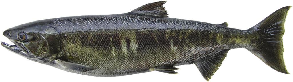
19 (RD), a depth measure independent of flow, was calculated at each pool by subtracting the pool tail depth from the max pool depth. Habitat measurements were made in 10 habitat units equally spaced downstream from the top point of the index. Measurements were equally spaced along a section of the index reach that was 20 times the length of the mean channel width (MCW) at the top of the index reach. The MCW selected for spacing was calculated from the average of three MCWs at the top of the index reach. Surveyors measured the wetted channel width at the top of the index reach again after walking upstream and downstream a distance equivalent to the first wetted channel width measurement. In some cases, the entire survey reach was too short to divide into 10 habitat units for measurement. In these cases, measurements were obtained from at least three locations in the reaches under 0.3 RM (e.g. sidechannels). Each index reach was assigned a size classification (side-channel, small, medium, large) based on proximity to the mainstem channel and BFW measures. Side-channels were the smallest classification with a BFW of 8 meters or less that were located off of a main stem river and thought to be breached during high water events in the fall. Small index reaches had BFW between 8 and 15 meters and were generally secondary or tertiary tributaries. Medium index reaches had BFW of 15 to 20 meters and were directly connected to the mainstem. Large index reaches had BFW of 60 m or greater and were mainstem river sections. General Survey Methods Surveyors were equipped with all necessary gear to safely conduct surveys and to ensure accurate counts, including polarized glasses and a brimmed hat to eliminate glare and increase in-stream visibility. Environmental data collected during each survey included water clarity, stream flow, riffle and pool visibility, direction surveyed, and weather. Water clarity was visually estimated as depth in feet the surveyor could see in the water column at the deepest point in the survey reach. Stream flow was recorded based on a qualitative 1 to 5 scale, where 1 indicates low flow/height and 5 indicates high flow/height for the reach. Riffle and pool visibility are separate, subjective measurements to indicate how well a fish could be seen spawning on a riffle/pool on a qualitative 1-5 scale, where 1 is excellent visibility and 5 is poor visibility for the reach. The direction being surveyed was either upstream or downstream. All boat strata were surveyed downstream. Most foot strata (86%) were also surveyed downstream; foot strata surveyed upstream were because of available access points or to determine upper extent/limit for distribution. The weather conditions were recorded as sunny/clear, cloudy/overcast, rain, or snow to indicate potential environmental factors impacting surveys. Surveyors were trained to accurately identify live and dead Chum, Chinook, Coho, and Steelhead which are holding and/or spawning during the same period with the same streams. Chum spawning is observed from the mid-october to mid-december based on QDNR and WDFW long-term surveyed reaches. Spawning Chum are identified by their olive green coloration with unique calico coloration (vertical bars along sides), white tips on the ventral and anal fins, the head shape of the males (large heads with large jaws), large canine-like teeth, no spotting on dorsal or tail, and narrow caudal peduncle. Females and some males can display a horizontal black stripe instead of the vertical bars. Chum are typically smaller than Chinook and larger than Coho. Chum holding in pools with Chinook and Coho can be identified by their darker coloration, but are hard to enumerate depending on the number of individuals in the pool. The surveyor made an estimate of the total number of Chum based on his/her observation of the activity in the pool. Redds were not used for the CMR analysis but were counted and tracked within the AUC reaches when possible. Area-Under-the-Curve (AUC) Index Reaches The purpose of the AUC index reaches was to obtain an estimate of fish-days for the selected AUC index reaches. The AUC method involved counts of live and dead Chum obtained in each AUC Grays Harbor Fall Chum Abundance and Distribution,

20 index reach between mid-october and early December. Surveys were conducted on a weekly basis unless weather conditions and/or stream flows made surveys impossible due to lack of visibility or safety concerns. Zero counts were obtained at the beginning and end of the data series. Live Chum were categorized as either holders or spawners. Holders were defined as fish that were not displaying spawning behavior, i.e., fish moving upstream, holding in pools. Spawners were defined as fish that were displaying spawning behavior on/near riffle areas, i.e. pairing up, actively digging. Several conversations between crew lead staff occurred before and during the beginning of the Chum spawning season to ensure spawner/holder classification was ubiquitous across all WDFW Chum Project and WDFW D17 FMS surveyors. Biological sampling of Chum carcasses was conducted in a portion of the AUC index reaches (Table 2). The first twenty carcasses of each one hundred carcasses encountered were sampled once: the species was determined, the caudal/tail section was intact (not previously sampled), and had scales available for collection. If the carcass could not be identified by species, it was recorded as species not determined (SPND) and not sampled. If the carcass was identified as a Chum and the caudal/tail region was missing, the carcass was not sampled, and recorded as did not sample. If the carcass was identified as Chum and it had a cut tail, it was recorded as a dead Chum previously mark sampled. Sport-caught Chum that were left along the bank were not included in the dead count or biological samples. Biological sampling included species identification, sex, length, and scales. Once biological sampling was complete, the tail was cut to identify that the carcass had been sampled. Further sampling (beyond 40/200) was conducted as time allowed. Therefore at least 40 Chum carcasses were sampled in reaches with more than 200 carcasses. Two scales were collected from the area posterior to the dorsal fin, anterior to the anal fin and above the lateral line, defined as the preferred area by the WDFW Scale Aging Lab. Scales were mounted on adhesive scale cards with a unique identifier for each fish that was also written on the field data card. Age of each fish was determined by the WDFW Scale Ageing Lab. Carcass Mark-Recapture (CMR) Index Reaches The purpose of the CMR index reaches was to obtain simultaneous and independent estimates of fish-days and spawner abundance in order to derive estimates of survey life. Additional information on survey life calculations is provided in a later section of this report (see analytical methods). Live counts provided the estimate of fish-days and carcass mark-recapture provided the estimate of spawner abundance. Similar to surveys in the AUC only index reaches, surveys in the CMR index reaches were conducted from mid-october through mid-december on a weekly basis unless weather conditions and/or stream flows made the survey impossible due to lack of visibility or safety concerns. Surveys began in October before Chum entered the study area (based on prior knowledge of the basin) and continued through mid to late December until no live Chum or taggable carcasses were observed for two consecutive weeks after the peak spawning period. Live and dead Chum were counted during each survey. Live Chum were categorized as holders or spawners, following the same method as used in the protocol outlined for AUC only index reaches. Data collection in CMR indexes also included carcass condition as well as carcasses that were tagged and released, and tagged carcasses that were recaptured from a previous week. Carcass condition was assigned on a scale of 1 to 5 (Table 4). All Chum carcasses with an intact tail were counted and examined for a carcass tag by lifting each operculum to determine whether a plastic tag was stapled to the inside. Previous tag status was recorded for operculum on both sides of the carcasses (one for each operculum). Previous tag status was recorded as the tag number, not present (if the operculum was present but no tag), or unknown (if the operculum area was missing). If a carcass was not able to be examined due to its location in the channel (e.g., deep pool, pinned to a log jam in fast flows), then it was counted as an unknown species with unknown tail status, and was not included in the total counts of dead Chum. Chum carcasses with a cut tail were not included in the dead count, because they were counted previously. Grays Harbor Fall Chum Abundance and Distribution,

21 Previously tagged carcasses were recorded as recaptures, their condition was scored, and their tails were cut to indicate whether they had been previously sampled. Untagged (maiden) carcasses were assigned as being in taggable or untaggable condition. Taggable condition meant that the carcass scored a 1, 2, or 3 on the qualitative scale (Table 4) and had both operculum attached. Untaggable condition meant that the maiden carcass scored a 4 or 5 on the qualitative condition scale or was missing one of the two operculum. Carcasses considered to be taggable has a square plastic tag with a four-digit number was stapled under the operculum on both sides of the fish. Each carcass had two tags (same number) and the placement of these tags under each operculum was not visible when looking at the carcass from a distance. Ensuring carcass tags were not visible helped reduce survey bias by necessitating each carcass was examined, and surveyors did not merely look for visibly tagged Chum. Surveyors measured the fork length in centimeters and designated sex as male, female or undetermined for each tagged carcass, then returned the carcass to the stream from where they were collected with their tails intact. Carcasses considered untaggable (i.e., had one or both of the operculum missing, or had a carcasses condition of 4 or 5), were counted and assigned as male, female or unknown. Tails were cut prior to returning them to the stream to indicate that the fish had been investigated and counted. A tagging rate was established for each CMR index reach to ensure survey completion during daylight hours. The tagging rate was selected at the beginning of the survey by the field lead based on the predicted number of carcass encounters and varied from week to week depending on carcass densities. When selecting a carcass tagging rate the field lead attempted to select a rate that could be maintained throughout the entirety of the survey and would maximize the number of fish to be tagged while completing the survey within daylight hours of a single day. The tagging rate (ex: 1 in 5 or 1 in 10) also ensured even distribution of tags throughout the survey. In the rare case where a survey could not be completed within one day, surveyors hung a flag at the stopping point and returned to the designated stopping point in order to complete the survey the following day. Table 4. Criteria for assigning carcass condition of Chum in the CMR index reaches. Condition Criteria 1 a Fresh, Clear eyes, Red gills 2 a Clear eyes, Firm flesh, White gills 3 a Cloudy eyes, Flesh starting to soften 4 Cloudy eyes, Flesh soft, Falling apart 5 b Partial carcass, Skeleton a Indicates taggable criteria. Both operculum needed to be present in order to tag the carcass. If one or both were not present, then the carcass did not get tagged and operculum status was recorded on the field card. b Only counted if the carcass could be identified as a Chum. Trap Returns Chum are encountered at two fish traps located within the Satsop sub-basin, one located on Bingham Creek and the other on the EF Satsop River. All Chum encountered at the Bingham Creek trap are enumerated and passed upstream to spawn, while Chum encountered at BCH are either lethally spawned or passed upstream. The Chum passed upstream are included in the total spawning population by adding the total number passed upstream to the final escapement estimate. The Bingham Creek trap at RM 0.9 has been in operation since 1982 and is used primarily for sampling adult Coho in the fall and the barrier portion is equipped with a downstream smolt trap during the spring months. The trap is operational year-round targeting Coho and Steelhead, but also encounters Grays Harbor Fall Chum Abundance and Distribution,

22 Cutthroat, Chinook, and Chum. Most wild fish (i.e., intact adipose fins) are placed upstream of the trap, except for some cases to retrieve coded-wire tags from wild Coho. The trap is monitored for adults moving upstream and is operated as the fish come into the system. The trap is checked daily during the fall. Each fish is netted individually, Chum are enumerated and the sex is determined for each individual before it is placed upstream. The only time the trap is not in operation is if there is a malfunction (usually occurs during high flow events). In this case, the trap is closed and not opened again until the trap is running properly. Chum passed upstream of the Bingham Creek trap were not monitored for fall back (Chum were not marked so fall back could not be determined). Fall back over the dam could be flow dependent with higher flows pushing more fish back over the dam. For Coho (operculum punched when put upstream) fall back is very low (3 fallbacks out of 641 put upstream in 2016). Chum could potentially have greater fall back than Coho as Coho are much stronger swimmers and could be in better condition this far upstream than Chum. The BCH trap is located on the EF Satsop River just upstream from the confluence of the EF Satsop River and Bingham Creek. The dam built at BCH on the EF Satsop River is approximately two and half meters tall and constitutes a complete barrier to Chum migration. To continue upstream all Chum must enter the fish ladder to the holding ponds. During the peak of the season the holding pond is sorted weekly. The Chum not removed for brood stock are enumerated and passed through an outlet pipe approximately 10 meters upstream of the barrier. The close proximity of the release tube to the barrier results in a fallback rate of approximately 5.3%. This rate was determined from a live mark-recapture study done in 2016 where live Chum collected and tagged at BCH, then recovered as carcasses on the spawning grounds. (Ashcraft et al. 2017). The total number of Chum received from BCH and included in the escapement estimate is not adjusted to compensate for fallback. Peak Counts The purpose of the peak counts in index and supplemental reaches was to determine the proportion of Chum spawning that occurred inside versus outside index reaches (Appendix A-2 and A-3). Surveys were conducted simultaneously in supplemental and index reaches during peak spawn time, providing a continuous view of spawning activity. During each survey, live and dead Chum were tallied by reach and live Chum were categorized as holders or spawners using the same protocol as the AUC and carcass mark-recapture reaches. No additional biological sampling was conducted in supplemental reaches. Supplemental and index reaches provided a continuous view of spawning activity during peak spawn time when the surveys were conducted simultaneously. Reaches within the foot strata survey type were surveyed by foot and reaches within the boat strata survey type were surveyed by pontoon or raft. The reach breaks between index and supplemental reaches along each tributary and along the main stem rivers were indicated with bright pink flagging with black dots at top and bottom of reach. Each supplemental reach was surveyed once during peak spawn time. To ensure consistency in data collection while accommodating for limited staff resources, peak counts were completed within a week time period within each survey type and sub-basin combination (e.g., peak counts in the Wynoochee foot strata were completed within one week). However, the weekly time periods for peak counts differed among survey type and sub-basin combinations (e.g., peak counts in the Wynoochee foot strata occurred on a different week than the Satsop foot strata). Ideally these surveys would be conducted during peak spawning to maximize the number of fish used in the calculations but surveys just prior to or after peak spawn timing were considered adequate if surveys needed to be adjusted based on river conditions. The peak spawn week was selected in advance using previous knowledge of the sub-basin available from the study completed in 2016 and WDFW D17 FMS and QDNR staff. Peak counts of live Chum in historical indexes reaches from the 1ast 10 years were observed on November 4th (statistical week 45) for the Wynoochee River and on November 12 th (statistical week 46-47) for the Satsop River. Advance preparation was also made to partition the supplemental areas into reaches that could be completed as Grays Harbor Fall Chum Abundance and Distribution,

23 daily surveys and to secure stream access permissions from landowners to enter these areas. Volunteers from the WDFW D17 FMS were recruited ahead of time to ensure enough surveyors were available to cover each sub-basin. Streams within the survey frame were prioritized at the beginning of the 2017 field season in anticipation of time constraints due to stream flows and high survey mileages associated with the peak counts. During the 2017 planning stages, streams with known Chum presence in 2015 and 2016 were given high priority for survey in Additional streams with a potential Chum presence were identified based on the WRIA catalog and scouting. These streams were designated medium or low priority for survey during the peak count week. If time allowed during the supplemental survey time frame, surveys were conducted in these additional tributaries. Upper Limit of Occurrence Supplemental surveys also provided field-based information on the upper limit of occurrence (ULO) of Chum spawning within tributaries of each sub-basin during the survey season. This information is vital to refining the survey frame used in the Chum project as well as the Chehalis Basin Upper Extent Project. The Chehalis Basin Upper Extent project is a basin-wide project focusing on the ULO of Chum, coho and steelhead with the goal of developing an empirical predictive model of Chum, coho and steelhead distribution in the Chehalis basin (E. Walther, WDFW, personal communication). Prior to the Chum spawning season, biologists from each project established a protocol for supplemental surveys that would satisfy the data needs of both projects. An ULO was determined for each supplemental reach that had Chum present and recorded using a hand-held GPS unit. When possible, streams were surveyed on foot starting at the mouth, or the lowest known Chum presence, and walking upstream. In the case where boats were necessary, surveys were started several RM upstream of suspected Chum presence. Surveys continued until one of the four criteria were met. 1) Walked 1 km without any Chum presence 2) Encountered a permanent barrier of 1.5m in height 3) Stream increases to a slope of 15% 4) Stream loses flow and goes sub-surface at the time of peak spawning Permanent barriers were primarily falls or cascades, and did not include beaver dams, log jams, landslides or culverts. The later are considered transient barriers since these can vary from year-to-year or are caused by anthropogenic influence. The height of the barrier is measured from the top of the water in the pool at the base to the top of the falls or cascade. Limiting stream gradient and barrier height are based on assumed Chum swimming and jumping ability (Powers and Osborne 1985, Resier et al. 2006). Chum presence was determined by identification of live or dead Chum within the stream, not redd identification. All live and dead Chum were enumerated during the survey. Redds and the presence of Chinook, coho and steelhead were recorded based on the surveyor s confidence in identification. Georeferenced locations included the beginning and end of each survey, the first and last Chum spotted and at any possible permanent or transient barriers. A description of the approximate barrier height and length was included and pictures taken if possible. Data Management Field data cards were completed in the field, and collected and regularly reviewed in-season by the project biologist. Cards were examined for any errors or missing information that was not recorded. Missing information was immediately addressed with the field staff. Georeferenced locations for each reach start and stop were added to this database as well. Data were summarized and entered into the Grays Harbor Fall Chum Abundance and Distribution,

24 WDFW SGS database. The SGS database held a subset of the information collected for this study. Therefore, the complete set of biological and carcass tagging data were entered into the District 17 Chum database in Microsoft Access Once all information was entered electronically the data cards were collected for the entire survey year were archived at the WDFW Region 6 office. Chum carcass survey data (biological sampling) were entered into the District 17 Biological Sampling database. Once entered, scale cards were copied, originals delivered to the WDFW Scale Ageing Lab to be aged, and final ages were entered into the District 17 Biological Sampling database. Analysis Biological Sampling Biological characteristics of Chum were summarized for all collected information including number of carcasses, sex composition, fork length and age composition. Chum Distribution Chum spawning distribution was summarized in two formats 1. ULOs were displayed by reach type (AUC, CMR, Supplemental) and by strata (foot, boat), and 2. Chum densities (fish per mile) displayed for all surveyed reaches (index, supplemental) during the peak spawning week. In addition, the proportion of spawning that occurred within the index reaches was calculated based on data collected during the peak spawning week when both index and supplemental reaches were surveyed. The proportion of spawning in the index reaches was calculated from live counts (holders, spawners) in all index reaches divided by live counts summed across all reaches (index, supplemental). The estimated proportion assumed a binomial variance: (1) n i ~ binomial(p i, N) where n i is the sum of live counts summed across all index reaches (i), p i is the proportion of spawning in the index reaches, and N is the sum of live counts summed across all index and supplemental reaches. The value of p i was calculated separately for each sub-basin and strata (foot, boat). Area-Under-the-Curve Calculations Counts of live Chum were used to estimate area-under-the curve in the AUC and CMR index reaches. Area-under-the-curve was estimated in fish-day units based on live counts and the number of days over which the live counts occurred. Data were organized by statistical week ensuring that a zero count occurred at the beginning and end of the time series and fish-days were calculated as (English et al 1992; Bue et al. 1998): (2) AAAAAA = 0.5 nn 1(tt dd tt dd 1 ) ( pp dd pp dd 1 ) where t d t d-1 is the number of days between surveys, p d is the number of live Chum observed on a given survey date, and p d-1 is the number of live Chum observed in the previous survey. Under this method, no fish are observed on the first (d = 1) or last survey (d = n). For most datasets, the count on the first and last survey week was zero; however, in the few cases where non-zero counts occurred at the beginning or end of the dataset, a zero count was added the week prior to the first surveyed week or after the last recorded survey for the purpose of calculation. Area-under-the curve was estimated for total live counts (holders, spawners) and for live counts of spawners only. Spawner Abundance in CMR Index Reaches Carcass tagging data were used to estimate spawner abundance in CMR index reaches. The carcass tagging data were analyzed with a Jolly-Seber (JS) estimator. The JS estimator is an open Grays Harbor Fall Chum Abundance and Distribution,

25 population mark-recapture model used to estimate abundance in situations where individuals immigrate and emigrate from the population over the course of study (Seber 1982; Pollock et al. 1990). The JS model has been successfully applied to mark-recapture data of live fish and carcasses in other salmon populations (McIssac 1977; Sykes and Botsford 1986; Schwarz et al. 1993, Bentley et al. 2018). When the estimator assumptions are met, the JS model produces an unbiased estimate of abundance with known precision. The JS estimator of spawner abundance estimate for each reach was based on the super population model (Schwarz et al. 1993) which was parameterized in a Bayesian framework. A conceptual schematic of the JS model is shown in Figure 1. A comprehensive description of this JS model, including summary statistics, fundamental parameters, derived parameters, and likelihoods can be found in Rawding et al. (2014) and Bentley et al. (2018). In this model, spawner escapement is the sum of gross births (i.e., arrival of new carcasses) that enter the system over the study period and includes the estimated number of carcasses present during each sampling period and the carcasses estimated to have entered the system after one sampling period and removed from the system prior to the next sampling period. Figure 1. WinBUGS schematic for Jolly-Seber abundance estimation developed by D. Rawding (WDFW). Parameters include sample period (t i ), probability of capture at sample period i (pp ii ), probability that a fish enters the population between sample period i and i +1 (bb ii ), probability that a fish alive at sample period i will survive and remain in the population between sample time i and sample time i + 1 (φ i ), population size at sample period i (N i ), number of fish that enter after sample time i and survive to sample time i +1 (B i ), and the number of fish that enter between sampling occasion i-1 and i (BB ii ). Total abundance (N) is the sum of BB ii over all sample periods. Under the Bayesian framework, parameters were calculated from the posterior distribution which calculated from a prior distribution and the data collected (posterior = prior * data). Samples from the posterior distribution were obtained using Markov Chain Monte Carlo (MCMC) simulations (Gilks et al. 1996) in the WinBUGS software package. WinBUGS implements MCMC simulations using a Metropolis with a Gibbs sampling algorithm (Spiegelhalter et al. 2003). Two chains were run with the Gibbs sampler in WinBUGS saving a total of 8,000 iterations of the posterior distribution of each parameter after a 2,000 iteration burn-in. A vague prior was used for the calculations (Bayes-LaPlace uniform prior). The sensitivity of the prior was based on the overlap between a uniform prior and the posterior distribution Grays Harbor Fall Chum Abundance and Distribution,

26 (Gimenez et al. 2009) and convergence was assumed for parameters with a Brook-Gelman-Rubin statistic value less than 1.1 (Su et al. 2001). Four potential JS models were evaluated using the Deviance Information Criteria (DIC) (Spiegelhalter et al. 2002). DIC is similar to AIC criteria in that both criteria include a model error estimate (posterior mean deviance) penalized for the number of terms in the model. Each of the four models estimated capture probability (p i - likelihood of detecting a carcass that was present during sample period i), survival probability (φ i - likelihood that a carcass present in one sample period i would remain in the stream until the next sample period), and entry probability (b* i - likelihood that a carcass would arrive in at a given sample period). The four models (e.g., ttt, stt, tst, sst) included a combination of static (s) or time varying (t) capture and survival probabilities among survey periods; the entry probabilities among survey periods were considered to be time varying in each of the three models. Survey Life Survey life (SL) in each CMR index reach was the area-under-the-curve divided by the JS spawner abundance estimate, where both estimates were independently derived for that index reach. This derivation of survey life represents BOTH the duration of time that live Chum were present AND the observer efficiency in the spawning index reaches. Area-under-the-curve values were treated as true values because no information on observer consistency was available, but JS spawner abundance was included as a distribution of values that incorporated the mean (µ N ) and standard deviation (σ N ) of the JS model estimate of spawner abundance. A Monte Carlo simulation (10,000 model simulations) provided the distributions of values for this calculation: (3) NN CCCCCC ~ nnnnnnnn(µ NN, σσ NN ) (4) SSSS = AAAAAACCCCCC NN CCCCCC For each CMR index reach, survey life was calculated separately for area-under-the-curve estimates based on total live counts (holder, spawners) and live counts for spawners only. Spawner Abundance in AUC Index Reaches Spawner abundance (NN AAAAAA ) in each AUC index reach was the area-under-the-curve divided by the survey life estimate, where the area-under-the-curve was calculated from live counts in the AUC index reach and survey life was selected from the CMR index reach of the corresponding stream size classification. Area-under-the-curve values were treated as true values because no information on observation consistency was available, but survey life was included as a distribution of values that incorporated the mean (µ SL ) and standard deviation (σ SL ) of the estimate (see equation 4). A Monte Carlo simulation (10,000 model simulations) provided the distribution of values for this calculation: (5) SSSS ~ nnnnnnnn(µ SSSS, σσ SSSS ) (6) NN AAAAAA = AAAAAAAAAAAA SSSS Spawner Abundance for Foot and Boat Strata Total spawner abundance was calculated separately for each watershed and strata. Total spawner abundance was the summed abundances in all index reaches (CMR, AUC) divided by the proportion of spawning (pp ii ) that occurred within the index reaches. The proportion of spawning that occurred in the index reaches was calculated from peak count data in index and supplemental reaches (see equation 1). This approach has been demonstrated to be effective for estimating population abundance of salmonids, Grays Harbor Fall Chum Abundance and Distribution,

27 especially if spawning numbers within the index reaches are a high proportion of total spawning in the strata (Liermann et al. 2015). Index reach abundances (NN ii ) were included as a distribution of values that incorporated the mean (µ N ) and standard deviation (σ N ) of the summed estimates (JS model for CMR indexes, equation 6 for AUC indexes). The proportion of spawning in index reaches was also included as a distribution of values that incorporated the mean (µ p ) and standard deviation (σ p ) of the estimated proportion (equation 1). A Monte Carlo simulation (10,000 model simulations) provided the distribution of values for this calculation: (7) NN ww,ss,ii = (NN CCCCCC ww,ss,ii, NN AAAAAA ww,ss,ii ) (8) NN ww,ss = NN ww,ss,ii ppww,ss,ii The final estimate was reported as abundance (mean of the simulated distribution), standard deviation (also calculated from the simulated distribution), and coefficient of variation (standard deviation divided by the abundance). Coefficient of variation is a measure of precision that is scaled to the magnitude of the values included in the estimate. Results Habitat Characteristics of Index Reaches Habitat measurements were successfully completed for 15 of the 24 index reaches in 2017 (Table 5). The remaining indexes were not surveyed due to time constraints at the beginning of the Chum spawning season. The size classifications designated to streams without measurements were based on knowledge from WDFW Chum Project staff of the relative BFW and characteristics of un-measured streams compared to similar streams with quantified habitat. Both Neil Creek (RM ) and Schafer Creek (RM ) were originally given a small size classification based on an average BFW, but carcass tagging was unsuccessful in these sections. With no ability to calculate survey life for small streams the small stream classification was combined with the medium size classification. This limited the categories to side-channel, medium and large. Of all index reaches, there were a total of 4 side-channels, 2 small channels, 12 medium channels, and 5 large channels. The average BFW for large streams was determined to be 45 meters or greater, and primarily consisted of mainstem sections. The medium size classification encompassed a range in average BFW from 13.8 to Although Schafer has an average BFW similar to side-channels, it is given a small size classification due to connectivity with the rest of Schafer Creek and its further distance from the mainstem Wynoochee river than other side-channels. Max residual depth increased with average BFW across all reaches and size classifications, with the deepest measurement of 1.81 meters located in the lowermost EF Satsop River section. Due to lack of distinguishable pools in side-channels max RD was not able to be measured. Grays Harbor Fall Chum Abundance and Distribution,

28 Table 5. Habitat measurements and size classification of index reaches used for estimation of Chum salmon abundance in the Wynoochee and Satsop sub-basins, Sub-basin Stream Reach Length (m) Average Bankfull Width (m) Average Thalwag Depth (m) Max Depth (m) Max Residual Depth (m) Wynoochee Wynoochee Large Wynoochee Large Size Class Schafer Creek d Medium Schafer Creek Medium Schafer Creek Medium Schafer Creek e Small Neil Creek e Small Satsop EF Satsop River Large EF Satsop River Large EF Satsop River Large EF Satsop River Medium MF Satsop River Medium MF Satsop River Medium Decker Creek Medium Schafer Slough c Side Channel Maple Glen c Side Channel Creamer Slough c Medium Dry Bed Creek ab Medium Decker Creek Medium Decker Creek Medium Decker Creek Medium Tributary Side Channel Tributary 0462A Side Channel a Creek partially, or completely dry when measurements were taken b Tributary remained almost completely dry through entire season c Long term chum index d Section is normally split at RM 1.3, but habitat measurements were taken continuously through both sections e Reaches were planned to be surveyed as CMR, but lack of carcass data resulted in these reaches being analyzed using AUC data. Survey life associated with medium size streams was used for analysis due to the lack of carcass tagging data from small streams in Biological Sampling For the purposes of this report, Chum biological data were summarized from the Satsop and Wynoochee sub-basins only, although data were collected more broadly from the Grays Harbor basin by the WDFW. For both the Wynoochee and Satsop sub-basins, Chum returned at three, four and five years Grays Harbor Fall Chum Abundance and Distribution,

29 of age (Table 6). In the Wynoochee, the majority of Chum returned at age four at 57% (n = 16), followed by age five at 29% (n = 8), with the smallest proportion returning at age three at 14% (n = 4) (Table 6). The age composition in Chum returning to the Satsop varied from the Wynoochee, with the majority returning at age three (41%, n = 66), followed by age four (33%, n=53) and the smallest proportion returning at age five (26%, n = 44) (Table 6). With only 28 Chum sampled in the Wynoochee, the small sample size could influence the ratios, resulting in a different age composition compared to the Satsop. The average fork length was 76 cm (±6, one standard deviation) for males and 69 cm (±5) for females in the Wynoochee (Table 6). Males had an average fork length of 79 cm (±5 SD) and a female average fork length of 71 cm (±4 SD) in the Satsop sub-basin (Table 6). The percentage of males and females in the Wynoochee was almost equal with 79 (52%) males and 74 (48%) females. In the Satsop more males were sampled than females, with 255 (56%) and 202 (44%) respectively. Table 6. Summary of scale age in years and fork length in cm for Chum from the Wynoochee and Satsop sub-basins, Basin Sex Scale Age (years) Sample Size Fork Length (cm) Sample Size Mean (±SD) Total Wynoochee M ±6 79 (52%) F ±5 74 (48%) Total 28 4 (14%) 16 (57%) 8 (29%) Satsop M ±5 255 (56%) F ±4 202 (44%) Total (41%) 53 (33%) 42 (26%) Distribution The Wynoochee survey frame included 89.0 river miles (RM, Table 7); however, 19.0 RM were not surveyed due to no visibility or access constraints resulting in 70.0 RM surveyed in 2017 (Figure 4). The Satsop survey frame included RM; however, 10.3 RM were not surveyed due to a combination of no visibility, access constraints, or time constraints resulting in RM surveyed in Details of the non-surveyed areas are provided in Appendix A-4. More river miles were surveyed by boat than by foot in both sub-basins. In the Wynoochee, 43.9 RM were surveyed by boat compared to 26.1 RM by foot, and in the Satsop 80.0 RM were surveyed by boat and 51.9 RM were surveyed by foot. Peak surveys were completed within a week time frame for each sub-basin and strata. A large rain event was predicted to raise river levels and decrease visibility starting November 12 th, and surveys of boat strata (main stem) were prioritized in case survey conditions in these areas were lost for the remainder of the season (Figure 2 and Figure 3). The Wynoochee boat strata was surveyed between November 6 th and 9 th and the Satsop boat strata was surveyed between November 7 th and 11 th. Wynoochee foot strata was surveyed between November 15 th and 22 nd, but the Satsop foot strata was not surveyed until December 1 st through 8 th due to a heavy rains and flooding that prevented safe access to the river between November 22 nd and 28 th (Figure 3). Grays Harbor Fall Chum Abundance and Distribution,

30 Table 7. Total river miles of known Chum distribution in each sub-basin that were surveyed and not surveyed in River miles are shown by strata and data collection method. Wynoochee Satsop Foot Boat Total Foot Boat Total AUC CMR Trap Counts a Supplemental Counts Total Surveyed Not Surveyed b Total Survey Frame a 100% capture traps are located on Bingham Creek at RM 0.9 and Satsop Springs Hatschery (EF Satsop River at RM 17.5). The areas above the Bingham Creek trap and Bingham Creek Hatchery on the EF Satsop River were not surveyed for upper extent/limit of Chum. This mileage is estimated based on the SalmonScape Chum distribution and District 17 local knowledge for Bingham Creek. The EF Satsop River mileage is based on surveys conducted in b Not Surveyed indicates river miles that were not surveyed in 2017 but were included in the survey frame. Chum were observed in 51.1 RM out of 70.0 RM surveyed in the Wynoochee sub-basin (Appendix A-2, Figure 5). The proportion of Chum within index reaches was 10% (n = 693/6,906) in the boat strata and 93% (n = 370/400) in the foot strata (Table 8). Based on peak counts, Schafer and Neil creeks appeared to contain the highest densities of Chum spawning within Wynoochee tributaries. Schafer Creek is the largest tributary below the Wynoochee dam and Neil Creek is a tributary to Schafer. During the 2017 peak spawning surveys, ULOs were observed at RM 6.1 in Schafer Creek and RM 0.5 in Neil Creek. The ULO in the Wynoochee main stem was further upstream than expected. Based on peak counts, a total of 316 live Chum were observed above the gorge and the uppermost Chum was recorded within 0.5 RM of the barrier fish trap, indicating that the gorge was not a barrier to Chum migration in Chum were observed in 81.0 RM of the RM surveyed in the Satsop sub-basin (Appendix A-3, Figure 6). The proportion of Chum observed within index reaches was 70% (n = 1,124/1,604) in the Satsop boat strata (Table 8). Surveys within the foot strata were delayed by high flows from storm events and ultimately occurred two to three weeks after peak (Figure 3) when there were few observations of live fish 0% (n = 0/8) within index reaches. However, carcass counts during peak surveys of the Satsop foot strata provided a more substantial sample size and 44% (n = 484/1,086) of Chum carcasses were observed within the index reaches in the Satsop foot strata. Based on peak counts, Decker Creek (EF Satsop River tributary) appeared to have the highest densities of Chum spawning within Satsop tributaries. Despite the high spawner densities, no Chum were observed in the upstream-most index in Decker Creek (RM ) and the ULO in Dry Bed Creek (tributary to Decker) was at RM 3.2. The ULO in the Satsop main stems were recorded at RM 30.4 in the WF Satsop River, RM 5.2 in Canyon River and 13.0 in the MF Satsop River. The ULO was not determined for Bingham Creek or the EF Satsop River; survey of these reaches were considered low priority for survey since numbers provided at the respective traps were sufficient for creating the Chum escapement estimate. Grays Harbor Fall Chum Abundance and Distribution,

31 Figure 2. Daily discharge for the Wynoochee River during the 2017 Chum survey season. Figure 3. Daily discharge for the Satsop River during the 2017 Chum survey season. Grays Harbor Fall Chum Abundance and Distribution,

32 Figure 4. Methods used to survey Chum salmon distribution in the Wynoochee and Satsop sub-basins. Methods include by reach type (AUC, CMR, Supplemental) and survey strata (foot, boat). Upper limit of occurrence indicated as the top of the reach. Reaches not surveyed but assumed to include Chum are shown. Grays Harbor Fall Chum Abundance and Distribution,

33 Figure 5. Chum density shown as fish counted per mile during a single week peak spawn survey in the Wynoochee and Satsop sub-basins. Reaches not surveyed but assumed to include Chum are shown. Blue stars indicate long-term Chum index reaches; Rose star indicates Tributary 0462 index reach. Grays Harbor Fall Chum Abundance and Distribution,