Stand Density Management for Optimal Growth. Micky G. Allen II 12/07/2015

Transcription

1 Stand Density Management for Optimal Growth Micky G. Allen II 12/07/2015

2 How does stand density affect growth? Langsaeter s Hypothesis (1941) Relationship valid for a given tree species, age and site Source: Daniel, T.W., J.A. Helms and F.S. Baker Principles of silviculture. Second Edition, Mc Graw-Hill.

3 Thinning and Growth: A full turn around Patterns for periodic annual total and merchantable volume increment (Gross volume) How is stand density defined? How is merchantable volume defined? Source: Zeide, B Thinning and growth: A full turnaround. J. For. 99(1):20-25.

4 Post-thinning relationship between growth and density Only a graphical representation Relative density? Total stem volume or merchantable volume? Source: Nyland, R.D Silviculture: Concepts and applications. Second Edition, McGraw-Hill. 682p.

5 Research Purpose Determine stand density that optimizes volume increment in loblolly pine plantations Use multiple operational studies Thinning vs. No Thinning Compare multiple definitions of stand density Commonly used measures of stand density Determine which is more correlated with volume increment Compare multiple definitions of volume increment Total vs. Merchantable Gross vs. Net

6 Data: Non-intensively managed plantations Thinning study established in 8-25 year old plantations Designed to examine thinning across a range of ages 186 permanent plots established across the natural range of loblolly pine Treatments: Unthinned control Light thin removing 30% of basal area Heavy thin removing 50% of basal area Management: Site preparation No genetic improvement No fertilization or weed control

7 Data: Intensively managed plantations Thinning study established in plantations 3-8 years old Stands thinned at a common point in stand development (45 ft, 13.7 m) 170 permanent plot locations across the natural range of loblolly pine Treatments: Unthinned control Light thin removing 30% basal area Heavy thin removing 50% basal area Management: Pruned, removing dead branches only Site preparation Genetically improved seedlings Fertilization and weed control

8 Data: Region Wide 19 Thinning Study Thinning and fertilization study established in plantations years old 8 permanent plot locations across natural range of loblolly pine Treatments: Thin to 1235 (500), 741 (300), 494 (200), and 247 (100) stems per hectare (acre) No fertilization or fertilization with N and P Four replications of each thin+fert combination at each location Management: Genetically improved seedlings Site preparation

9 Data: Spacing Study Trials designed to examine effects of different planting densities established in 1983 Four locations established in Virginia and North Carolina 3 replications of study design at each location Base design: Grid with four spacings (4, 6, 8, 12 ft) (1.2, 1.8, 2.4, 3.6 m) Spacing varies in two-dimensions for a total of 16 plots Ex: 4x4, 4x6, 4x8, 4x12, etc. In this work only the initial planting density was considered 4x6 = 6x4 = 1815 stems/acre 9 initial planting densities 2722, 1815, 1361, 1210, 907, 680, 453, and 302 stems/acre 6727, 4484, 3363, 2989, 2242, 1681, 1494, 1121, and 747 stems/hectare

10 Definitions of Stand Density Stems per Hectare (SPH) Basal Area per Hectare (BPH, m 2 /ha) Relative Spacing Diameter: RSD = 10,000/SPH d q, d q = quadratic mean diameter (m) Height: RSH = 10,000/SPH H d, H d = dominant height (m) Stand Density Index * Diameter: SDID = SPH 25 d q Height: SDIH = SPH 30 H d Volume: SDID = SPH 0.65 v , v = mean tree volume (ft 3 ) * Parameter estimates from: Burkhart, H.E Comparison of maximum size density relationships based on alternate stand attributes for predicting tree numbers and stand growth. Forest Ecology and Management 289(0):

11 Volume Estimation Total volume (ft 3 /acre) * Unthinned: V u = D 2 H, D = diameter(in), H = height (ft) Thinned: V t = D 2 H Merchantable volume (ft 3 /acre) * Unthinned: MV u = V u exp d D Thinned: MV t = V t exp d D Volumes converted to metric (m 3 /ha) Pulpwood: Trees in the 13 cm DBH class and greater to 7.6 cm top(d) Sawtimber: Trees in the 20 cm diameter class and greater to 15.2 cm top (d) * Volume equations from: Tasissa, G., H.E. Burkhart, and R.L. Amateis Volume and Taper Equations for Thinned and Unthinned Loblolly Pine Trees in Cutover, Site-Prepared Plantations. Southern Journal of Applied Forestry 21(3):

12 Growth Definition Net Productivity: Standing volume + Volume removed in thinning Gross Productivity: Net + Volume of mortality Productivity = Periodic annual increment (PAI) PAI = Volume 2 Volume 1 Time 2 Time 1 Measurement periods ranged from 2 to 3 years

13 What kind of pattern? V a1 V a Density exp( a 2 Density) 0 Increasing Optimum Stand Density

14 Hypothesis Testing PAI a1 a 0 Density exp( a 2 Density) Test of hypothesis: Ho : Optimum pattern between volume increment and stand density HA : Increasing pattern between volume increment and stand density or Ho : all coefficients are significant HA : all coefficients, except, are significant

15 Results: Definitions of Growth and Density Measures Based on diameter were more correlated with growth BPH, RSD, SDID Consistently explained the most variation in volume increment (20-30%) Net and Gross growth had similar relationships in most cases

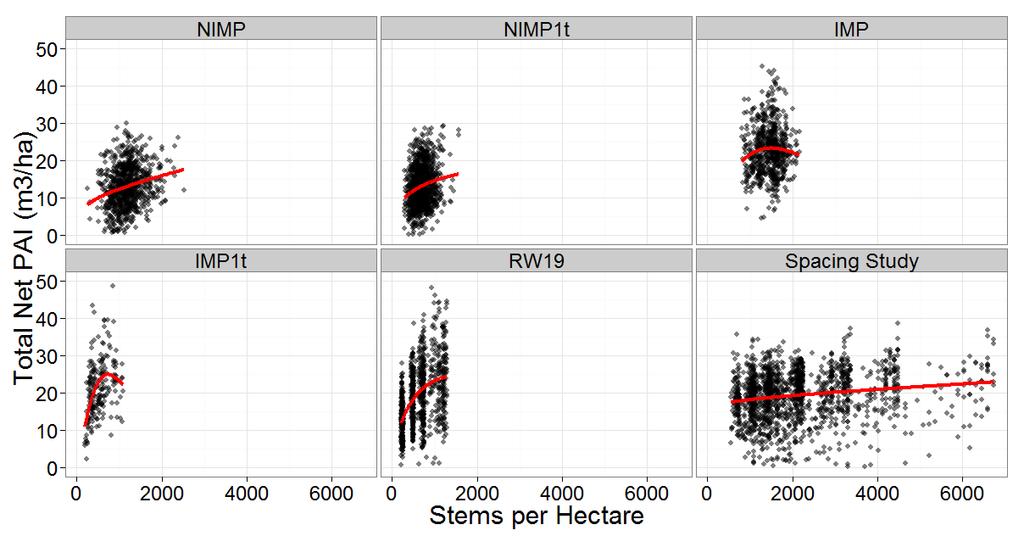
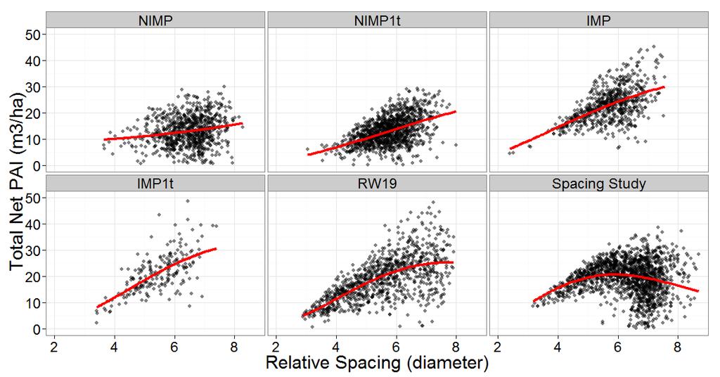
16 Results for Total Volume Increment

17

18

19

20

21

22

23

24

25 Results: Is there a stand density that optimizes total volume increment? Dataset NIMP PAI Density SPH BPH RSD RSH SDID SDIH SDIV Gross Net 291 NIMP1t Gross Net IMP Gross Net IMP1t Gross Net RW19 Gross Net Spacing Study Gross Net Hypothesis test concluded an optimal relationship Density values that optimize total volume increment

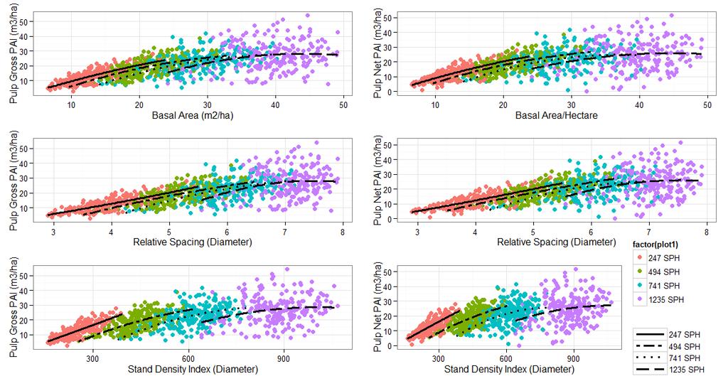
26 Results for Pulpwood Volume Increment

27

28

29

30

31

32

33 Results: Is there a stand density that optimizes pulpwood volume increment? Dataset PAI Density SPH BPH RSD RSH SDID SDIH SDIV NIMP Gross 3.31 Net NIMP1t Gross 75.8 Net IMP Gross Net IMP1t Gross Net RW19 Gross Net Spacing Study Gross Net

34 Results for Sawtimber Volume Increment

35

36

37

38

39

40

41 Results: Is there a stand density that optimizes sawtimber volume increment? Dataset PAI Density SPH BPH RSD RSH SDID SDIH SDIV NIMP Gross Net NIMP1t Gross Net IMP Gross 356 Net 350 IMP1t Gross Net RW19 Gross Net Spacing Study Gross Net

42 Conclusions Results of hypothesis test were different depending on the dataset, measure of growth, and measure of density Approach was inconclusive at determining the relationship between growth and density Stand density measures based on diameter (BPH, RSD, and SDID) consistently explained the most variation in volume increment (20% 30%) No consistent solution between these measures

43 Different Approach #1 Zeide (2004) argues that optimal density cannot be determined as in the previous manner Relating volume increment as a function of density alone does not account for the effects of age and average tree size (quadratic mean diameter) Age: as stands age any gaps in the canopy created by mortality become more difficult to fill by the residual stand Volume increment can only be optimized when the canopy is full Any gaps in the canopy reduce the total amount of light interception Average tree size: Stands at similar densities can have largely different average diameters Average diameter and density can determine diameter increment which is related to volume increment Source: Zeide, B Optimal stand density: A solution. Canadian Journal of Forest Research 34(4):

44 Formulating a model: Define the volume of an average tree Using a local volume equation v = αd q β Using the combined variable equation v = αd q 2 H d Where v = mean total tree volume (m 3 ) D q = quadratic mean diameter (cm) H d = mean tree height (m) α,β = parameters to be estimated

45 Formulating a model: Differentiate to obtain individual tree volume increment equations dv = αβd β 1 dd q dt q dt dv = α 2D dd q dt qh d + D dt q 2 dh d dt Where dv dt = individual volume increment (m3 / year) dd q dt = diameter increment (cm / year) dh d dt = height increment (m / year)

46 Formulating a model: Multiply volume increment of average tree by Stems per Hectare dv dt = SPH αβd q β 1 dd q dt dv = SPH α 2D dd q dt qh d + D dt q 2 dh d dt Where dv dt = volume increment per hectare (m3 / hectare / year)

47 Formulating a model: Add modules to account for the effects of age and density dv dt = SPH αβd q β 1 dd q dt exp γ age exp( Dens ) δ dv = SPH α 2D dd q dt qh d + D dt q 2 dh d dt exp γ age exp( Dens ) δ Where γ,δ = parameters to be estimated

48 Formulating a model: Formulate SPH as a function of commonly used measures of density BPH = BA tree SPH SPH = BPH = BPH 2 2 = c BPH d BA q tree d q c RSD = 10,000/SPH d q SPH = c RSD 2 d q 2 SDID = SPH 25 d q SPH = c SDID d q

49 Formulating a model: Replace SPH in volume increment equations dv = α BPH D dt q c dd q dt exp γ age exp( BPH ) δ dv = α dt RSDθ c D dd q q dt exp γ age exp( RSD δ ) dv = α SDID D dt q c dd q dt exp γ age exp( SDID ) δ

50 Results: Is there a stand density that optimizes volume increment? Both local and combined variable formulations with all measures of density resulted in optimal relationships between density and volume increment (for all measures compared here) In all cases the optimal density was well outside the commonly held theoretical maximum SDI for loblolly pine in the southern U.S. of 450, as defined by Reineke (1933) which equates to inch trees per acre or centimeter trees per hectare. Using this approach it appears that maximum volume increment occurs near the maximum observed densities

51 Different Approach #2 Use the RW19 data Individual plots were thinned to a common number of stems per hectare Treatments: 1235, 741, 494, and 247 residual SPH Spacing Study data Nine different planting densities 6727, 4484, 3363, 2989, 2242, 1681, 1494, 1121, and 747 SPH Fit 2 nd degree polynomial to each thinning treatment and planting density PAI = B0 + B1 Density + B2 Density 2 Useful for determining if different relationships exist among treatments

52 Results from the RW19 Study

53

54

55

56 Results: Fitting 2 nd degree polynomial to thinning treatments Dens. Thinning Total Gross PAI Pulpwood Gross PAI Sawtimber Gross PAI Treatment R 2 OptD OptP R 2 OptD OptP R 2 OptD OptP BPH 247 SPH SPH SPH SPH RSD 247 SPH SPH SPH SPH SDID 247 SPH SPH SPH SPH OptD = optimum density, OptP = PAI at which density is optimized

57 Results from Spacing Study

58

59

60

61 Conclusions

62 Total Volume Increment Maybe Langsaeter (1941) was partially right Volume seems to become near optimal over a wide range of densities although not necessarily constant A decrease in volume production at higher levels of density may not be observable Before a reduction in volume increment can occur stands self-thin Adjustment to Langsaeters Hypothesis

63 Merchantable Volume Increment Relationship between pulpwood volume increment and density is similar to that of total volume increment Merchantable volume increment can become optimal Depends on: Initial planting density Thinning Intensity

64 Is this the final answer?

65 Questions?