Carbon in the Forest Biomass of Russia

Transcription

1 Carbon in the Forest Biomass of Russia Woods Hole Research Center R.A. Houghton Tom Stone Peter Schlesinger David Butman Oregon State University Olga Krankina Warren Cohen Thomas K. Maiersperger Doug Oetter

2 Context Temple in the remote Southeastern Tibet.

3 Context 1. What is the C balance of the northern mid-latitudes? 2. What are the mechanisms responsible for the current (and future) C balance? a. Are forests growing faster? (physiology) b. Are more forests in a regrowth phase? (age structure past disturbances - LCLUC)

4 Questions: How much carbon is in the biomass of Russian forests? How has that amount changed in the last decade(s)?w

5 What would the map look like in 2000? 1990 Forest Cover Map of USSR

6 Approach

7 Approach Russian forest inventory data for training Landsat ETM + (growing stock -> C/ha) Landsat ETM + for training MODIS MODIS for scaling to all Russia

8

9 Stratify Russian forests into ~15 ecoregions by Geo-regions (4): European Russia, Western Siberia, Eastern Siberia, Far East Vegetation zones (5): Northern, central, southern taiga, temperate forest, forest steppe

10

11 Forest Inventory Data

12

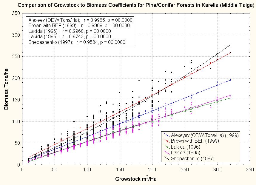
13 Total Biomass predicted from growing stocks by age by eco-region by species (group)

14 Training Landsat data with Inventory Data

15 Videl (inventory polygon) data overlaid with Landsat ETM+ data

16 Fitted function In theory i

17 In fact Observed & predicted biomass for individual videls (polygons)

18 Inventories acquired, processed,

19 Another test (coarser resolution). Compare larger forest inventory unit (lesnichestvo) with Landsat-derived estimates of... Forest area Average C/ha

20 Scaling up with MODIS

21 Approach Russian forest inventories for training Landsat ETM + Landsat ETM + for training MODIS MODIS for scaling to entire Federation

22 But wait

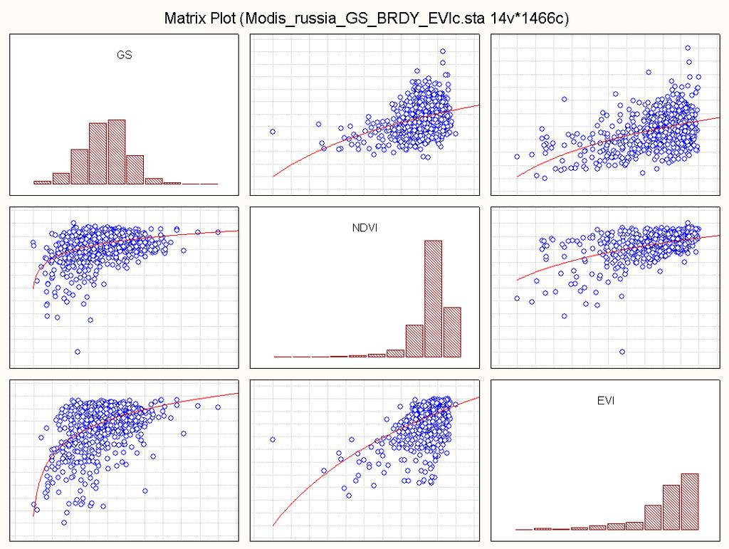
23 An Alternative Approach At a more aggregated (coarser) scale (leskhoz), MODIS may be a reasonable predictor of biomass C (??)

24 Leskhoz boundaries ~1880 Leskhozes in the Russian Federation

25 MODIS surface reflectance (MOD43B4) (BRDF product)

26 Leskhoz boundaries ~1880 Leskhozes in the Russian Federation

27

28 Chang W. Lee A Kurdish fighter prayed in near the Iraq-Iran border, after American and Kurdish forces ousted an Thank you

29

30

31 1990 Forest Cover Map of USSR

32 Geo-Ecoregion stratification for sampling Highly generalized vegetation zones of the FSU based on the work of Kurnaev. Forested zones - green. The mixed forest (light green). The brown zone - forest steppe, which grades south into steppe. The four regions of Russia to be studied are colored and are (l to r), European-Urals, West Siberia, Central Siberia, and Eastern Russia.

33

34

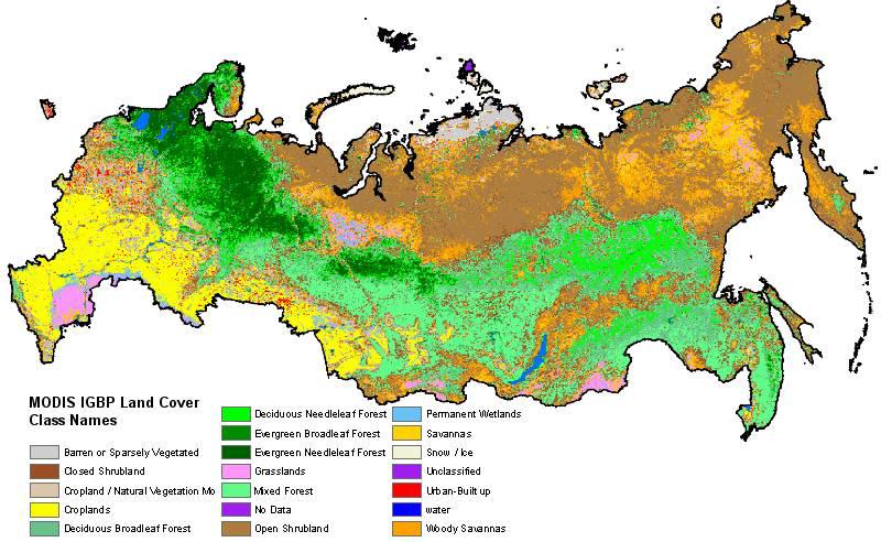
35 GLC 2000 Forest Cover for Russia (8.3 million Km 2 ) MODIS IGBP Forest Cover for Russia (6.5 million Km 2 )

36 Spatial Analysis for the Development of a Russian Biomass Map Iterative Iso-clustering of Digital Data: ERDAS: Unsupervised Classification of Atmospherically corrected DN s into forest and non-forest land cover classes Non-forest includes all agriculture, urban etc. The recoding of the digital data is based off of the percent composition data given within the Forest Inventory. Recoding the raw DN s into a forest sub-type classification: -Pine -Spruce -Mixed Conifer -Deciduous -Mixed Forest Training plot derived from this classified data coded 1-5 for each forest type Supervised Classification: ( Maximum likelihood Classification) Derive classified images that are specific to the forest types: Pine Spruce Mixed Conifer Deciduous Mixed Forest Have in hand separate spatial datasets. These datasets are used to separate the image into batches of data that reflect each forest type.

37 Split Forest Inventory Data set into a Testing and a Training Dataset: Model 1 Model 2 Analysis of Raw DN s Perform Transformation on all bands Square Root Square Log Inverse Log To determine if non-linear relationships exist and can be corrected for using various techniques. Bands Selection and Statistical Analysis Done By Species For the Development of A Russian Biomass Map Create Correlation Plots for all bands and all transformations against Vegetation data: (Biomass). The correlation plots between raw DNs and biomass are used to determine if non-linear relationships exist, and then the transformations are created and re-plotted to see if they correct for the non-linearity. R-Square: Develop a ranking mechanism to tell which combination of bands/transformations produces the strongest correlations with the Biomass Values Rule: (Due to Co-linearity between Bands) Use two bands from the visible spectrum Bands 1 or 2, and 3 Use two bands from the infrared spectrum Bands 4, and 5 or 7 RMA Technique: Slope = (sign of correlation +/-) Sdy / SDx x = LANDSAT (CCA Index) y = BIOMASS (Inventory) Intercept = mean Y - slope * meanx Pred = slope (LANDSAT) + intercept RMSE = square root ( average (residual squared) ) ) Canonical Correlation Analysis: Evaluate the four bands and the inventory biomass values using a CCA technique. Derive Canonical Index of landsat values: Reduce Major Axis Regression: (RMA) Used to perform a regression between the inventory biomass values and the summed Canonical index values CCA INDEX Derivation: The index is created by summing the Input bands/transformations, that have been Standardized about the mean and multiplied By the canonical coefficient for that band From the RMA we obtain an equation that is then multiplied against the original CCA Biomass Indices to create a biomass layer that is species specific.

38

39