EXECUTIVE SUMMARY. 1.0 Introduction. 2.0 Distribution System Infrastructure TOWN OF ADDISON WATER MASTER PLAN

Transcription

1

2 EXECUTIVE SUMMARY 1.0 Introduction In May 2014, the Town of Addison authorized Bury, Inc. to perform a Water Master Plan Study. The goals of this project were to develop a robust steady-state and extended period water model, evaluate the integrity of the existing water distribution system, and craft a Capital Improvements Project Plan. Recommended improvement projects will serve as a foundation list for future design, construction, and financing of facilities required to meet Addison s water demands as a result of existing needs, 5-year-out projected growth, and build-out projected growth. 2.0 Distribution System Infrastructure The Town of Addison water distribution system includes the following major system components: Pipelines, valves, and hydrants Six (6) Dallas Water Utilities (DWU) interconnections: two (2) primary delivery supply facilities and four (4) standby or emergency facilities Three (3) Carrollton emergency interconnections One (1) Farmers Branch emergency interconnection Surveyor Pump Station (4.0 MGD flow capacity) and Ground Storage Tank (2.0 MG storage capacity) Celestial Pump Station (20.0 MGD flow capacity) and Ground Storage Tank (6.0 MG storage capacity) Addison Circle Elevated Storage Tank (1.0 MG storage capacity) Surveyor Elevated Storage Tank (1.5 MG storage capacity) SCADA and Control Systems The pipeline, valve, and hydrant components of the Town of Addison s water system were located by land survey and mapped using a combination of survey data, previous GIS data, and record drawings review. January 14,

3 3.0 Water Model Development Bury developed a computer model of the Town of Addison water system by importing existing water system data into the water distribution system modeling software Bentley WaterGEMS V8i. The ModelBuilder tool within WaterGEMS was the means by which the building of the base physical infrastructure (i.e. pipes and junctions) of the water model was accomplished. The supply facilities, pump stations, and tanks (EST & GST) were manually added to the water model. Inputting operational settings for both initial conditions and extended period simulations was accomplished using the controls component in WaterGEMS to establish condition alternatives for the hydraulics present within the system. Water demands were allocated to the water model based on user-type. A combination of Thiessen Polygons (from WaterGEMS) and GIS manipulation (spatial join) was used to develop a shapefile in GIS containing the water model junctions/nodes to which the corresponding demands were allocated. The allocated demands were then re-imported into WaterGEMS using the LoadBuilder tool and the demands were assigned to the corresponding junction in the water model. Average Daily Demand (ADD), Maximum Daily Demand (MDD), and Peak Hourly Demand (PHD) for Existing conditions, 5-year Period conditions, and Master Buildout conditions were developed and are summarized in Table ES-1. January 14,

4 Table ES-1 Current and Projected Addison Water Demands Year ADD (MGD) MDD (MGD) PHD (MGD) Existing (2015) yr Period (2020) Buildout As a basis for the Extended Period Simulations (EPS), a Diurnal Demand Factor Pattern was generated and inputted into the water model. Chlorine residual data was obtained for the timeframe: January 2015 to September 2015 in order to effectively evaluate a correlation between water age and chlorine residual for the purposes of model evaluation. Development of the water age portion of the Water Model was to enhance the hydraulic model to obtain a nonspecific measure of overall water quality, evaluating storage tank turnover impacts on the distribution system s water quality, and providing evaluation of the current flushing program. 4.0 Water Model Calibration & Validation In order to more accurately represent and predict real-world conditions, calibration and validation of the water model was performed. Fire flow tests were conducted in the field and stand as the basis by which the water model was calibrated against real-world conditions. Scenarios and specific demand alternatives were set up in the water model using boundary conditions and water demands recorded in the field at the time of the fire flow tests. Minor adjustments were made to the water model such as changing Hazen-Williams C-values, pipe materials, and pipe connections until the model results were within a tolerable variance from the field test results. The calibration and validation process also included, because of some discrepancies between the recorded SCADA data and the provided pump curves, a number of iterations to obtain accurate pump curves that accurately represented the real-world functioning of the pumps. Multiple GST draw-down tests were conducted at each pump station to acquire real-world pump flow data with which to compare against the pump curves that had been January 14,

5 provided. Adjustments were made to the pump curve definitions in the water model to correct any discrepancies. 5.0 Hydraulic Analysis Hydraulic analysis of the water distribution system included two (2) phases: Phase 1: Steady- State Analysis and Phase 2: Extended Period Simulations & Water Age Analysis. As the base for evaluating the hydraulic conditions of the water distribution system, design criteria for minimum & maximum allowable velocities, head-losses, pressures, and minimum fire flow rates were specified for normal steady-state (static) and fire flow demand scenarios. A summary of the hydraulic design criteria can be seen below. Table ES-2 Hydraulic Design Criteria Demand Condition Hydraulic Criteria ADD, MDD, PHD MDD + FF Max Velocity (fps) 7 7 Max Head Loss (ft/ft) 4/1000 (or 0.004) N/A Min Pressure (psi) Max Pressure (psi) Min Specified Fire Flow (gpm) N/A 1000 Steady-state model runs were conducted for twelve (12) demand alternatives by which the hydraulic design criteria were evaluated; the twelve (12) demand alternatives are a function/multiplication of the three (3) timeframes (Existing, 5-yr Period, and Buildout) and the four (4) demand conditions (ADD, MDD, PHD, and MDD+FF). The Steady-State Hydraulic Analysis represents a snapshot in time of the water distribution system in which the established initial conditions of the water model greatly influence what happens and what doesn t happened during a model run. Thus, careful caution was taken to establish accurate worst-case initial conditions. The steady-state model runs combined with requests from Addison were used to develop the initial CIP list. January 14,

6 Among other things, the extended period simulations were used in Phase 2 of the water modeling to re-evaluate and refine the CIP plan. An additional two (2) CIP options were determined in order to meet hydraulic criteria. Also, the EPS model was used to evaluate the functional operational controls currently in use within the Town, analyze in greater depth the existing storage and pumping capabilities, and establish recommendations for emergency management by performing model runs for different, potential emergency scenarios. The water age portion of the Water Model was used to enhance the hydraulic model so that water age analyses can provide a simple, nonspecific measure of overall water quality, evaluate storage tank turnover impacts on the distribution system s water quality, and provide evaluation of the current flushing program. Two (2) additional CIP options were determined during the analyses to reduce water age in certain portions of the system. Water age analyses were then combined with an evaluation of chlorine residual data for January September 2015 to assist in developing a general picture of overall water quality within the system and to serve as the basis for the development of multiple recommendations to combat poor water quality. January 14,

7 6.0 Capital Improvement Projects (CIP) Plan From the hydraulic analyses, a water infrastructure capital improvement projects (CIP) plan was developed to ensure hydraulic design criteria within the system are met so that Addison can continue to deliver great water distribution services. An initial list of CIP options was created by analyzing the ADD, MDD, PHD, and MDD + FF scenarios in the water model for existing, five-year (2020), and build-out conditions. Any areas or components that failed to meet specific design criteria were improved by a combination of line upsizing, replacing aging infrastructure, and adding new infrastructure. The list of CIP options was prioritized using risk-based analysis and can be seen in the table below. Table ES-3 CIP Risk, Cost, & Priority Summary Option No. Priority Length (~ LF) Option Description (including location) Replacing 8-in CI with 8-in PVC Water Main (Greenhaven Village Shopping Ctr at Intersection of Marsh Ln & Spring Valley Rd) Replacing 8-in DI with 8-in PVC Water Main (Prestonwood Place Shopping Ctr near Intersection of Beltline Rd & Montfort Dr) Upsizing 8-in CI to 10-in PVC Water Main (Running N to S from Beltline Rd to George H.W. Bush Elementary) Replacing 8-in CI with 8-in PVC Water Main (Intersection of Beltway Dr & Beltline Rd - Beltway Office Park) Upsizing 6-in CI to 8-in PVC Water Main (Lake Forest Drive) Upsizing 6-in Unk to 8-in PVC Water Main (Apartment Complex at NE Intersection of Addison Rd and Westgrove Dr) Upsizing 16-in DI to 24-in RCCP (Intesection of Belt Line Rd and Quorum Dr) Upsizing 16-in RCCP to 24-in RCCP (in Belt Line Rd between Addison Rd and Quorum Dr) Upsizing 8-in DI to 10-in PVC Water Main Near 36-in to 8-in Connection (SE Corner of Village on the Parkway) Upsizing 6-in PVC to 8-in PVC Water Main (Shadwood Apartments - Sydney Dr & Marsh Ln) Upsizing Short Connection from 6-in to 8-in (North of Beltline on Quorum) Upsizing 8-in PVC to 12-in PVC Water Main (The Wellington Square - Southern Edge of Addison) Upsizing 8-in PVC to 10-in PVC Water Main (Quorum Office Building #2) CoF LoF Risk Factor Improvement Cost Estimate (Current) $566, $264, $953, $611, $460, $516, $292, $845, $69, $551, $24, $26, $81,178 January 14,

8 Upsizing 8-in PVC to 12-in PVC Water Main (Excel Telecommunications Service Center to Addison Rd) Upsizing 6-in Unk to 8-in PVC Water Main (Glenn Curtiss Dr & Addison Rd) Upsizing 8-in Unk to 10-in PVC Water Main (The Madison Dallas North Parkway) Upsizing 6-in Unk to 8-in PVC Water Main (Quorum Office Building #2) New 6-in PVC Water Main Loop (Talisker Apartments - off of Vitruvian Pkwy) Upsizing 8-in PVC to 10-in PVC Water Main (Lateral off of Quorum Dr) Upsizing 12-in PVC to 16-in DI Water Main Connection Between 36-in & 12-in Main (South of Beltline on Quorum) New 8-in PVC Water Main Loop (Excel Telecommunications Service Center to Addison Rd) Upsizing 8-in PVC to 12-in PVC Water Main (Millenium Phase I - NW Intersection of Arapaho & DNT) New 8-in PVC Water Main Loop (FedEx Store Airport Pkwy) New 10-in PVC Water Main Loop (One Hanover Park Offices to Excel Pkwy along DNT) Upsizing 6-in PVC to 8-in PVC Water Line for Lateral (Off of Claire Chennault Street) New 12-in PVC Water Main Loop (Apt. Complex in NW Corner of Town) 7.0 Conclusions and Recommendations $106, $43, $22, $27, $429, $50, $25, $238, $18, $298, $341, $105, $821,486 In conclusion, the recommendations and deliverables provided within this report are based upon sound engineering and modeling principles. However, while comprehensive, they are not allinclusive of the many layers of intricacy present within Addison s water distribution system and at this point are at best a fair assessment and representation of the water infrastructure assets at this time. Even though Addison s distribution system is robust and the mapping, water model, capital improvement projects plan, and water master plan report provide a comprehensive evaluation of the system, there is always room for continual improvement. Wrapped up within these future considerations is the recommendation that the Water Master Plan report developed herein be updated regularly (recommended annually at a minimum) to accommodate for any changes, variations, or new infrastructure development made to the water distribution system. January 14,

9 Table of Contents 1.0 INTRODUCTION GENERAL OBJECTIVES/SCOPE OF WORK DISTRIBUTION SYSTEM INFRASTRUCTURE PIPELINES, VALVES, AND HYDRANTS SUPPLY FACILITIES DWU Interconnections Primary Delivery Facilities Standby Delivery Facilities Carrollton Interconnections Farmers Branch Interconnections SURVEYOR PUMP STATION AND GROUND STORAGE TANK CELESTIAL PUMP STATION AND GROUND STORAGE TANK ADDISON CIRCLE ELEVATED STORAGE TANK SURVEYOR ELEVATED STORAGE TANK SCADA AND CONTROL SYSTEMS WATER MODEL DEVELOPMENT MODEL SETUP AND ASSUMPTIONS Physical Component Development Pipes, Junctions, and Skeletonization Supply Facilities (Reservoirs) Tanks (EST & GST) Pump Stations System Operational Settings WATER SYSTEM DEMANDS Existing Water Demand Development (Historical) ADD Development - Meter Records MDD Development - Pump Station Flow Data MinDD Development - Pump Station Flow Data Peaking Factors & PHD Development January 14,

10 3.2.2 Allocation Process Diurnal Demand Pattern Population & Land Use Future Water Demand Development WATER AGE INFORMATION WATER MODEL CALIBRATION AND VALIDATION FIRE FLOW TESTS Locations & Maps Data Collected Results PUMP CURVE EVALUATIONS ITERATIVE CALIBRATION PROCESS HYDRAULIC ANALYSIS DESIGN CRITERIA PHASE 1: STEADY-STATE HYDRAULICS PHASE 2: EXTENDED PERIOD SIMULATIONS Calibration & Validation Steady-State CIP Plan Evaluation Operational Controls Evaluation Storage and Pumping Evaluation Emergency Management Evaluation PHASE 2: WATER AGE & QUALITY ANALYSIS General System Water Quality Water Quality Improvement Recommendations CAPITAL IMPROVEMENT PROJECTS (CIP) PLAN COST ESTIMATES RISK-BASED ANALYSIS IMPACT FEE ANALYSIS CONCLUSION AND FUTURE CONSIDERATIONS APPENDICES January 14,

11 List of Figures Figure 2.1 Existing Water System Figure 3.1 User-Type Map Figure 3.2 Diurnal Demand Pattern Figure 3.3 Future Development Map Figure 4.1 Fire Flow Test Locations Figure 5.1 MinDD Water Age Map Before CIP Figure 5.2 MinDD Water Age Map After CIP Figure 6.1 Capital Improvement Projects Plan Map Figure 6.2 Risk-Based Analysis Graphical Depiction January 14,

12 List of Tables Table 2.1 Statistical Breakdown of Town of Addison Pipelines Table 2.2 Surveyor Pump Station Data Table 2.3 Celestial Pump Station Data Table 3.1 Tank Physical & Operating Range Attributes Table 3.2 Pumping Facilities Summary Table 3.3 Demand User-Types Table 3.4 Existing ADD, MDD, Peaking Factor, and PHD Summary Table 3.5 Existing ADD, MDD, Peaking Factor, and PHD Summary Table 3.6 Existing ADD, MDD, Peaking Factor, and PHD Summary Table 4.1 Fire Flow Test Data Table 5.1 Hydraulic Design Criteria Table 5.2 Statistical Summary of Steady-State CIP Identified Table 5.3 Statistical Summary of Extended Period Simulation CIP Identified Table 5.4 Operational Control Settings Summary Table 5.5 TCEQ Storage Tank Capacity Requirements Table 5.6 Existing Storage Tank Analysis Table 5.7 TCEQ Pumping Capacity Requirements Table 5.8 Existing Pumping Capacity Analysis Table 5.9 Emergency Management Scenarios Table 6.1 Identified Capital Improvement Projects (CIP) Table 6.2 Estimated Water System Construction Unit Prices Table 6.3 Consequence of Failure (CoF) Criteria Weightings Table 6.4 Likelihood of Failure (LoF) Criteria Weightings Table 6.5 Likelihood of Failure Sub-Criteria for Rating Pipe Material Example Table 6.6 CIP Risk, Cost, & Priority Summary Table 6.7 Impact Fee Comparison Summary January 14,

13 List of Appendices Appendix A Emergency Interconnection Record Drawings Appendix B Pump Station Layouts Appendix C Pump Curves Appendix D Detailed Fire Flow Test Location Maps Appendix E Proposed Operational Control Setting Parameters Appendix F Chlorine Residuals (Jan. - Sept. 2015) Appendix G CIP Plan Priority Matrix Appendix H Risk Based Analysis Calculations & Data Appendix I Proposed Impact Fee Schedule Appendix J Impact Fee Analysis Calculations & Data January 14,

14 Abbreviations ADD Average Daily Demand CI Cast Iron CoF Consequence of Failure DI Ductile Iron DWU Dallas Water Utilities EPS Extended Period Simulation GPD Gallons per Day GPM Gallons per Minute HGL Hydraulic Grade Line LoF Likelihood of Failure MDD Maximum Daily Demand MGD Million-Gallons per Day MinDD Minimum Daily Demand NCTCOG North Central Texas Council of Government PCCP Pre-Stressed Concrete Cylinder Pipe PHD Peak Hourly Demand PRVs Pressure Reducing Valves PS Pump Station PVC Poly-Vinyl Chloride ROW Right-of-Way SCADA Supervisory Control and Data Acquisition TDH Total Dynamic Head Unk Unknown WAA Water-Age Analysis January 14,

15 1.0 INTRODUCTION 1.1 General In May 2014, the Town of Addison authorized BURY, Inc. to perform a Water Master Plan Study. The goals of this project were to 1.) Develop a robust steady-state and extended period simulation water model, 2.) Evaluate the integrity of the existing water distribution system, and to 3.) Craft a Capital Improvements Plan by prioritizing infrastructure projects based on their timeline of development, critical nature, and the Town of Addison s immediate needs. Recommended improvement projects will serve as a foundation list for future design, construction, and financing of facilities required to meet Addison s water demands as a result of existing needs, 5-year out projected growth, and build-out projected growth. 1.2 Objectives/Scope of Work The scope of work for this Water Master Plan Study includes the following objectives: Water Model Development Field Testing and Water Model Calibration Water Modeling Phase 1: Steady State Hydraulic Analyses of Average Day Demand (ADD), Maximum Day Demand (MDD), Peak Hour Demand (PHD), and Maximum Day Demand plus Fire Flow (MDD + FF) for three timeframe conditions: o Existing System Conditions o 5-yr Period System Conditions o Master Build-Out System Conditions Water Modeling Phase 2: Extended Period Simulations to evaluate the following: o Steady-State CIP Plan o System Operational Controls o Storage and Pumping Capacities o Emergency Management Scenarios January 14,

16 Water Modeling Phase 2: Water Age Analyses to evaluate/provide the following: o General System Water Quality o Water Quality Improvement Recommendations Develop Capital Improvement Project Plan by identifying, recommending and prioritizing projects needed to meet hydraulic design criteria and incorporating the Town of Addison s existing troublesome maintenance locations 2.0 DISTRIBUTION SYSTEM INFRASTRUCTURE The Town of Addison operates their water system within one pressure plane. Infrastructure in a water distribution system generally consist of pipelines, valves, hydrants, pump stations, ground storage tanks (GST), elevated storage tanks (EST), and normally water treatment facilities. However, the Town of Addison has no water treatment facilities because they buy wholesale treated water from DWU. The wholesale treated water is delivered to the Town of Addison at two locations: Surveyor Pump Station and Celestial Pump Station. As important as it is to understand the system infrastructure and it s interconnected functioning for the purpose of physical operation and maintenance it is just as critical for water modeling because a water model is only as good as the base physical components it is built upon. Thus, as a means of elucidation this section of the report will discuss the existing infrastructure and the process undertaken to gather, collect, develop, and compile physical infrastructure data into maps and databases for the ultimate purpose of building the water model which will be discussed in the following section. See Figure 2.1 for an overall layout map of Addison s existing distribution system infrastructure. January 14,

17 Legend UT UT $1 $K $1 Addison Town Limits Addison Parcels Addison Storage Tank DWU Storage Tank Carrollton Emergency Connection Farmers Branch Emergency Connection DWU Standby Delivery Facility "C` DWU ROF Meter Water Lines Addison Carrollton DWU NTTA Private Farmers Branch (Abandoned) Addison Circle Elevated Storage Tank Surveyor Pump Station & Ground Storage Tank Beltwood Pump Station & Ground Storage Tank Surveyor Elevated Storage Tank Celestial Pump Station & Ground Storage Tank 0 1,500 3,000 Feet Figure 2.1 Town of Addison Existing Water System I

18 2.1 Pipelines, Valves, and Hydrants The ability to effectively model a water system depends largely on the accuracy of the base physical infrastructure data used to perform the initial build of the model. For increased accuracy, land surveying was used to pick up the geographic locations and ground elevations of valves and hydrants. Next, the piping was mapped using a combination of survey data, previous GIS data, and record drawings review. The prior GIS data was used as the initial approximation of the location and physical attributes of the infrastructure. The land survey data acquired in junction with a record drawing review was used to accurately improve, update, and map the existing infrastructure using a connect-the-dot approach between valves and hydrants, particularly focusing on the pipe lines themselves to ensure proper sizing, connectivity, material, and age of pipe. The attribute table for the water lines was populated with detailed information acquired largely from the record drawings themselves, such as installation year, record drawing name, owner, and physical features such as size, material, and etc. The elevation data acquired by the land survey for the valves and hydrants themselves was used later during the calibration process to evaluate hydraulic grade lines for the purpose of comparing against the model. The ground elevations within the city range from 496 feet to 686 feet. Addison pipeline infrastructure is significant, consisting of over 100 miles of pipe ranging in size from 42-inch diameter mains to 3/4-inch diameter service lines. The list of pipeline materials present in Addison includes: copper (CU), ductile iron (DI), cast iron (CI), reinforced concrete cylinder pipe (RCCP), pre-stressed concrete cylinder pipe (PCCP), Steel, and poly-vinyl chloride pipe (PVC). See Table 2.1 below for a statistical breakdown of the Town of Addison s pipelines. January 14,

19 Table 2.1 Statistical Breakdown of Town of Addison Pipelines Pipeline Material Approximate Length (Linear Feet) Percentage of Total Length CU 20, % DI 30, % CI 34, % PCCP & RCCP 22, % Steel (at Celestial PS) 185 < 1.0% PVC 289, % Unknown (Unk) 136, % Also, present within Addison is DWU owned infrastructure including approximately 7 miles of pipeline ranging in size from 6 inches to 84 inches and the Beltwood Reservoir Facility which is slightly northwest of the Addison Rd and Belt Line Rd intersection. Clear distinction of Addison owned versus DWU owned infrastructure has been made and can be seen in Figure 2.1: Existing Water System. The water model developed included only Addison owned infrastructure. 2.2 Supply Facilities Just as critical as the proper physical data of the pipelines, valves, and hydrants is the proper physical data of the supply connections present within Addison. Supply interconnections discussed in this section include DWU, Carrollton, and Farmers Branch and both wholesale supply facilities and emergency facilities. Addison has a total of six (6) connection locations with DWU: two (2) primary delivery supply facilities and four (4) standby (emergency) facilities. Addison, also, has three (3) emergency interconnections with Carrollton and one (1) with Farmers Branch. The main intent of the emergency interconnections is to provide supply either to Addison from DWU, to Addison from DWU through Carrollton or Farmers Branch, or to Carrollton and Farmers Branch from DWU through Addison in the case of an emergency or pump station failure. The January 14,

20 two (2) primary delivery facilities operate as the main, normal operation supply connections for the Town of Addison. Please see Figure 2.1 for a map detailing the supply facility locations DWU Interconnections Addison purchases wholesale treated water from DWU at a contractual rate of 11.0 MGD, of which 9.8 MGD is delivered through the Celestial Pump Station connection and 1.2 MGD is delivered through the Surveyor Pump Station connection. These two (2) interconnections constitute the primary delivery facilities for DWU to Addison. As mentioned above, there are also four (4) standby (emergency) connection locations between Addison and DWU which, per the wholesale treated water contract with Dallas, are referred to as standby delivery facilities Primary Delivery Facilities The Surveyor and Celestial Rate of Flow Controlled (ROFC) metering stations were installed and placed into operation in 1976 and 1988, respectively. They have a maximum combined delivery flow capacity of 24.0 MGD. The Surveyor Rate of Flow Controlled (ROFC) metering station is located at Surveyor Blvd. and is equipped with a 12 venturi meter capable of delivering 4.0 MGD. The Celestial ROFC metering station is located at 5510 Celestial Rd. and is equipped with a 20 venturi meter capable of delivering 20.0 MGD. Although the ROFC metering stations are sized for up to 24.0 MGD, the current wholesale contract with DWU is capped at 11.0 MGD. The two (2) primary delivery connection meter vaults are owned by DWU Standby Delivery Facilities Standby Delivery Facilities serve as emergency supply connections and thus act as integral components of a robust water infrastructure system. The four (4) standby delivery facilities have a maximum combined delivery flow capability of approximately 18.9 MGD. The first standby delivery facility consists of an 8 FM (fire service) meter with a maximum delivery capability of 4.0 MGD and is located at the northeast corner of Addison Road and Belt Line Road. The second standby delivery facility consists of a 6 FM (fire service) meter with a maximum delivery capability of 2.3 MGD and is located at the southeast corner of Dallas Parkway and Westgrove January 14,

21 Road. The third standby delivery facility consists of a 10 Turbine meter with a maximum delivery capability of 6.3 MGD and is located in the Celestial Road ROW directly north of the Celestial PS. The final standby delivery facility consists of a 10 Turbine meter with a maximum delivery capability of 6.3 MGD and is located slightly east of the southeast corner of Dallas Parkway and Belt Line Road. See Figure 2.1 for a map of the Standby Delivery Facility locations. Also, see Appendix A for copies of the record drawings for each Standby Delivery Facility Carrollton Interconnections As mentioned above, there are three (3) interconnections with Carrollton that serve as an alternate emergency connections. Each interconnection is bi-directional which allows emergency water supply for either the Town of Addison or the City of Carrollton. Based on record drawing review and discussions with operations staff the location of the three (3) interconnection facilities have been identified to be 1) slightly north of the Surveyor Blvd and Lindbergh Dr intersection, 2) at the NE corner of the Wiley Post Rd and Midway Rd intersection, and 3) on the SE corner of the Midway Rd and Kellway Circle intersection. See Figure 2.1 for a map of the Carrollton Interconnection locations Farmers Branch Interconnections There is one (1) interconnection with Farmers Branch that serves as an alternate emergency connection which is, also, bi-directional. Once again, based on record drawing review and discussions with operations staff the location of the Farmers Branch connection has been identified to be on Beltwood Pkwy E a bit south of Belt Line Rd on the west side of Beltwood Pkwy E. on the edge of the Addison and Farmers Branch City boundary. 2.3 Surveyor Pump Station and Ground Storage Tank The Surveyor Pump Station and Ground Storage Tank function as a single facility consisting of three (3) centrifugal booster pumps and a 2.0 MG Ground Storage Tank. The facility was formally constructed and put into operation in The Ground Storage Tank is a 26 foot tall concrete January 14,

22 tank with a diameter of 120 feet. The inflow pipe into the tank is a 12-inch diameter line and the overflow pipe diameter is 12-inches. The outflow pipes feeding into the pump station are two (2) 24-inch diameter lines. The three (3) pumps in the pump station consist of two (2) different pump curves. See Table 2.2 below for a breakdown of the pumps. The pumps act in parallel and have a total capacity of approximately 9850 GPM and a firm capacity of 6000 GPM. The total capacity is the summation of all of the pumps operating point capacities, and the firm capacity is the total capacity minus the largest pump. More detail regarding the operational criteria of the Surveyor Pump Station will be discussed in the proceeding sections. See Appendix B depicting the Surveyor & Celestial Pump Station layouts. Table 2.2 Surveyor Pump Station Data Pump # Pump Flow (gpm) TDH (feet) Impeller " " " Total Capacity (gpm): 9850* Firm Capacity (gpm): 6000** * Total Capacity = Summation of all of the pumps operating point capacities ** Firm capacity = total capacity minus the largest pump 2.4 Celestial Pump Station and Ground Storage Tank The Celestial Pump Station and Ground Storage Tank function as a single facility consisting of five (5) two-stage vertical turbine booster pumps and a 6.0 MG Ground Storage Tank. The facility was formally constructed and put into operation in The Ground Storage Tank is a 26 foot tall concrete tank with a diameter of 206 feet. The inflow pipe into the tank is a 36-inch diameter line and the overflow pipe are (2) 24-inch diameter lines. The outflow pipes feeding into the pump station are two (2) 42-inch diameter lines. The five (5) pumps in the pump station consist of three (3) different pump curves. See Table 2.3 below for a breakdown of the pumps. The pumps act in parallel and have a total capacity of approximately 26,200 GPM and a firm capacity of 19,200 GPM. The total capacity is the summation of all of the pumps operating point capacities, and the firm capacity is the total capacity minus the largest pump. More detail January 14,

23 regarding the operational criteria of the Celestial Pump Station will be discussed in the proceeding sections. See Appendix B depicting the Surveyor & Celestial Pump Station layouts. Table 2.3 Celestial Pump Station Data Pump # Pump Flow (gpm) TDH (feet) Impeller " " " " Total Capacity (gpm): 26,200* Firm Capacity (gpm): 19,200** * Total Capacity = Summation of all of the pumps operating point capacities ** Firm capacity = total capacity minus the largest pump 2.5 Addison Circle Elevated Storage Tank The Addison Circle Elevated Storage Tank is an iconic part of the Town of Addison s water infrastructure system. The EST was built and put into operation in The tank has a 1.0 MG capacity and is 150 feet tall with a diameter of 74 feet. The inlet/outlet pipe size is 24-inches, and the overflow pipe diameter is 12-inches. More detail regarding the operational criteria of the Addison Circle EST will be discussed in the proceeding sections. 2.6 Surveyor Elevated Storage Tank The newest addition to the Addison water distribution system was built and put into operation in The tank has a 1.5 MG capacity and is approximately 177 feet tall with a maximum diameter of 90 feet. The inlet/outlet pipe size is 24-inches, and the overflow pipe diameter is 16- inches. More detail regarding the operational criteria of the Surveyor EST will be discussed in the proceeding sections. 2.7 SCADA and Control Systems A key to any well-functioning water distribution system is an effective SCADA and Control System. Proper understanding of the SCADA system and more particularly the varied operational Control January 14,

24 Systems present within the Town is key to developing an accurate water model. All of the primary supply facilities within Addison have sensors for operation and control at each facility. Refer to the Town of Addison Public Works, Utilities Division Operations Manual for details of the SCADA system operations and controller information. 3.0 WATER MODEL DEVELOPMENT This section will discuss the steps and efforts taken to develop and build the Water Model. Subsections to be included herein include Physical Component Development, System Operational Criteria Inputting, Population (discussing and developing correlations between population and demand), and Water System Demand development. 3.1 Model Setup and Assumptions The software used by the team for water modeling was Bentley WaterGEMS V8i which has a number of dynamic features, tools, and capabilities. The initial model setup included the created GIS map data, infrastructure data, and operational criteria. Once created the initial model was reviewed to verify that the data was inputted/inserted correctly and that the data inputted/inserted made sense in comparison to real-world conditions. The subsections discussed herein are essentially presented in order by which they were developed in the model Physical Component Development Included in this section is a summation of the steps used to import and input the physical infrastructure data: pipes, junctions, supply facilities, pump stations, and tanks (EST & GST) which were acquired and mapped as discussed in Section 2.0 Distribution System Infrastructure. The ModelBuilder tool within WaterGEMS was the means by which the building of the base physical infrastructure (i.e. pipes and junctions) of the water model was accomplished. The supply facilities, pump stations, and tanks (EST & GST) were manually added to the water model. January 14,

25 Pipes, Junctions, and Skeletonization The first step of creating the water model was an initial build (i.e. importation) of the GIS Addison Waterline shapefile data using the ModelBuilder tool. Upon the initial build of the model, pipe connections (junctions) were automatically generated at all pipe endpoints using spatial relationships between the pipelines. Next, the process of skeletonizing the model, trimming out the less critical pipes and junctions, was used to simplify the model. The general assumption made was that pipes 6-inches in diameter or smaller were the least critical unless they functioned as a critical connectivity or loop within the system in which case they were maintained. Thus, all pipes and associated junctions 6-inches in diameter or smaller that did not play a critical role in the connectivity of the water model were removed from the model. The Skeletonization process helped greatly in simplifying the model. Then, once the model was skeletonized, a detailed, iterative review, refinement, and clean-up process was conducted to ensure the pipelines and junctions accurately reflect real-world connectivity of the infrastructure. Upon completion of the connectivity review and refinement, the junctions were exported to a Shapefile in order to assign elevations by using AutoCAD Civil 3D to project the junction points to the NCTCOG surface acquired from Addison. Elevations of the junctions in the water model are crucial to mimic accurately the hydraulic conditions of the real world. Once the junctions were assigned elevations, the junction nodes were then reimported into the Water Model along with the skeletonized water model using the ModelBuilder tool. At this point, the building of the base physical components of the water model were completed and relatively finalized. However, it should be noted that while progressing forward with the model development process, further gaps and holes in the physical structure of the model were discovered and corrected in kind. For instance, after many other components were added to the Water Model it was discovered that there were some connectivity missing between some of the pipes within the model and that there were also three (3) pressure reducing valves (PRVs) missing, as well. Essentially, it is upon this physical component base that the supply facilities, pump stations, tanks, system operational controls, and demand allocation water model components were built. January 14,

26 Supply Facilities (Reservoirs) In the case of this Water Model, the definition to be used for supply facilities will be the supply connections with the surrounding cities and it will be represented in the model as a reservoir with a physical elevation set to the hydraulic grade line present in the respective water system at that connection point. As discussed previously in Section 2.2 Supply Facilities, there are two (2) primary delivery facilities which act as the water supply connections for the Water Model, and there are an additional eight (8) standby delivery facilities, four (4) with DWU, three (3) with Carrollton, and one (1) with Farmers Branch that have been included/added to the Water Model to allow for modeling and analysis of emergency scenarios within the model. It should be noted that at this time, in accord with the scope of work of this project, no hydraulic data regarding the Carrollton and Farmers Branch connections has been acquired and there is no way of accurately incorporating them into any modeling scenarios; however, if hydraulic data is ever collected it would be simple to input into the model and run analysis of the effects. The two (2) DWU primary and four (4) DWU standby delivery facilities are located within DWU s North High Pressure Plane which has an established hydraulic grade line (HGL) of feet based on the overflow height of the elevated storage tanks present within this DWU pressure plane. Thus, an elevation of feet was assigned to all six (6) DWU delivery facilities. In the Water Model, DWU facilities (reservoir components) were connected to the respective ground storage tanks and subsequently pump stations for the two (2) primary delivery facilities and via connections to metering vaults represented by isolation valves for the eight (8) standby delivery facilities. From a water model perspective, the supply facility (reservoir) acts as a constant, steady supply of water feeding the system; whereas, the tanks fluctuate in junction with the pumps in a corollary fashion to mimic real-world hydraulic grade line conditions. January 14,

27 Tank Name Tanks (EST & GST) As discussed previously in Section 2.2 Supply Facilities, there are four (4) tanks within the Town of Addison s water distribution system. There are two (2) GSTs, each located at a Pump Station site: Surveyor GST and Celestial GST. There are, also, two (2) ESTs: Addison Circle EST and Surveyor EST. These tank components were added and connected to the system using the tank feature in WaterGEMS, and the physical data of the tanks was set to match the information discussed in Section 2.2. Operation related physical inputs were added to the tanks such as initial water levels/elevations, low-water level/elevation alarms, maximum elevations, and high-water level/elevation alarms were set. These physical inputs become critical when performing Extended Period Simulation (EPS) model runs. See Table 3.1 below for a summary of the physical inputs for each tank. Ground Elev. (ft) Table 3.1 Tank Physical & Operating Range Attributes Operating Range Type Elev. (Base) (ft) Elev./Level (Minimum) (ft) Elev./Level (Initial) (ft) Elev./Level (Maximum) (ft) Elev./Level (Low Alarm) (ft) Elev./Level (High Alarm) (ft) Vol. Full (Input) (MG) Surveyor GST 603 Level Celestial GST 594 Level Surveyor EST Elevation Addison Circle EST 639 Elevation Dia. (ft) Install Year Pump Stations The two (booster) pump stations owned and operated by the Town of Addison are the Surveyor PS and Celestial PS. Description of the physical nature of these two (2) pump stations and the pumps present within them was discussed in Section 2.3 and 2.4. See below in Table 3.2 a summary of the pumps operating points. See Appendix C for a copy of each pump curve. Unfortunately, the process of acquiring the correct pump curves for each pump was a bit more tedious than originally anticipated; an iterative process to obtain the correct, real-world pump curves was conducted and is discussed in Section 4.2 Pump Curve Evaluations. January 14,

28 Table 3.2 Pumping Facilities Summary Pump Capacity (gpm) TDH (ft) Celestial Pump 1 7, Celestial Pump 2 3, Celestial Pump 3 7, Celestial Pump 4 2, Celestial Pump 5 7, Surveyor Pump 1 3, Surveyor Pump 2 3, Surveyor Pump 3 3, The pumps were added to the Water Model using the pump and pump station features in WaterGEMS and connected up to the appropriate pipes in the base model. The pump curve data was inputted using the multiple point pump definition and then they were assigned to the appropriate pump. Operational control criteria were then acquired and established for each pump which is further discussed in the next section System Operational Settings Included in this section is a quick discussion on the initial conditions and a brief summary of the system operational settings used in the model. The operational settings were developed in accord with the Town of Addison s Public Works, Utilities Division Operations Manual and have been established to mimic Operational Settings A from the manual which have been updated to match the new system conditions including Surveyor Elevated Storage Tank. During the first phase of the water modeling, steady-state hydraulic analyses were conducted in which initial conditions became critical because each run was simply a snapshot in time, and thus, the results depended greatly on which pumps were on or off and what the Elevated Storage Tank levels were. Throughout the steady-state hydraulic analyses, initial conditions were established to mimic the likely real-world worst-case conditions which vary depending on the water demand scenario. The initial condition variations were determined based upon established trends within the Town of Addison, discussion with Town staff regarding general operational norms for January 14,

29 particular times of the year, and general adherence to the Operational Settings A detailed in the Operations manual. During the second phase of the water modeling, extended period simulations were conducted in which functioning Operational Settings became necessary to accommodate changes in the operations of the system over time. For instance, the response of tank levels, pumps on/off, and general reactionary relationship between all of the components system is one aspect being analyzed during the extended period simulations. Inputting operational settings was accomplished using the controls component in WaterGEMS to establish condition alternatives in relation to the hydraulic conditions present within the system. Refer to Section for a discussion on the proposed Operational Controls developed using the model. 3.2 Water System Demands Accurate depiction of water system demands is critical to effectively modeling a water distribution system. The scope of Phase 1 of the water modeling (Steady-State) included the development of Average Daily Demand (ADD), Maximum Daily Demand (MDD), and Peak Hourly Demand (PHD) for Current/Existing conditions, 5-year period conditions, and Master-Buildout conditions. The scope of Phase 2 of the water modeling (Extended Period Simulation) included the development of a diurnal demand pattern. The development, calculation, and allocation of the aforementioned demand conditions will be discussed within this section Existing Water Demand Development (Historical) ADD Development - Meter Records The basis for the development of the existing ADD was the historical customer metered (monthly) demand records for the years 2012, 2013, and These meter records were acquired from Addison via the water billings department. Initial evaluation of the metered demand records yielded discovery of a variety of discrepancies which required Data Trimming (data cleanup). January 14,

30 Upon completion of the Data Trimming, ADDs were calculated by User Type per meter. Further discussion of these two efforts will be discussed within this subsection Data Trimming The 2012, 2013, and 2014 historical customer metered (monthly) demand records were provided as raw tabular data in the form of an excel table for each year that, when analyzed in more detail, yielded discovery of a variety of discrepancies such as more/less values of data than the number of months in a year, numerous demand records having a value of zero, and multiple records per meter/customer. Due to these discrepancies in the demand records, the accuracy of the data for the purpose of calculating existing ADD was considered suspect. Thus, a thorough review of the data was conducted and the invalid, inconsistent, and discrepant records were corrected or deleted altogether if they were discovered to be wrong. This process of Data Trimming was fairly tedious and time-consuming, but it was necessary for assuring the accuracy of the data from which the existing ADDs were calculated Demand Calculations How the demands were to be allocated in the Water Model dictated the form and method by which demands were calculated. It was assumed that demand records for the years would be a fairly representative time period for reflecting the existing demands for the year In excel, each year s records were sorted, filtered, and organized based first upon user-type, then by customer address, and then by meter. The user-types were provided in the historical customer metered (monthly) demand records and are as seen below. January 14,

31 Table 3.3 Demand User-Types User-Type Description COMLG Commercial Large COMSM Commercial Small H_M Hotel & Motel INDLG Industrial Large INDSM Industrial Small IRRLG Irrigation Large IRRSM Irrigation Small MFLG Multi-Family Large MFSM Multi-Family Small SCH School SF Single Family TOWN-WA* Town Owned Facilities TOWN-IR* Town Irrigation (Parks, Medians, Public Spaces, etc.) *The UserType provided by Addison was actually just TOWN, but it was delineated into TOWN-WA and TOWN-IR by adding the UTILITYTYPE filter of WA (general water) and IR (irrigation water) Once the data was properly sorted, calculations were performed for each year (2012, 2013, and 2014) to generate Town-Wide ADDs and user-type per meter specific ADDs which were then subsequently averaged and summarized to attain the existing (2015) ADDs. The following sections discuss how the existing MDDs were developed, how peaking factors were calculated, and how the peaking factors were used to calculate the MDD and PHD for each user-type per meter MDD Development - Pump Station Flow Data In order to calculate ADD to MDD peaking factors (equal to MDD divided by ADD), baseline MDDs needed to be developed for each year. The calculation of a MDD for each year was accomplished through the analysis of the 2012, 2013, and 2014 Town of Addison Daily Pump Station Daily Activity CP records for the Celestial PS and Surveyor PS. Just as with the ADD, it was assumed that the analysis of pump station discharge records suffices as a representative reflection of existing (2015) MDDs. The data was entered into excel, analyzed, and summarized to calculate the Town-Wide MDD per year in million-gallons per day (MGD). January 14,

32 MinDD Development - Pump Station Flow Data For the purpose of evaluating Water Age, Minimum Daily Demands (MinDD) were calculated. In order to calculate ADD to MinDD peaking factors (equal to MinDD divided by ADD), baseline MinDDs needed to be developed for each year. The calculation of a MinDD for each year was accomplished through the analysis of the 2012, 2013, and 2014 Town of Addison Daily Pump Station Daily Activity CP records for the Celestial PS and Surveyor PS. Just as with the ADD, it was assumed that the analysis of pump station discharge records suffices as a representative reflection of existing (2015) MinDDs. The data was entered into excel, analyzed, and summarized to calculate the Town-Wide MinDD per year in million-gallons per day (MGD) Peaking Factors & PHD Development At this point, progressing forward with the calculation of peaking factors and ultimately PHDs was fairly simple. The peaking factor for ADD to MDD was calculated for each year (2012, 2013, and 2014) and then averaged across the three years to acquire the final peaking factor of During the Steady-State Phase 1 of Water Modeling a diurnal demand pattern was not developed. Thus, a PHD could not be generated by which to calculate a MDD to PHD peaking factor; thus, a peaking factor of 2.00 was assumed based on industry norms. Using the ADD to MDD peaking factor of 2.03 for and the MDD and PHD peaking factor of 2.00 the following demands were calculated. Also, for the purpose of evaluating Water Age, an ADD to MinDD peaking factor of 0.44 was calculated. A summary of the calculations discussed within this section can be seen in Table 3.4. Equation: MDD = 2.03 x ADD Equation: PHD = 2.00 x MDD Equation: MinDD = 0.44 x ADD January 14,

33 Table 3.4 Existing ADD, MDD, Peaking Factor, and PHD Summary Per Meter Averages Gal/Day ADD MDD PHD ADD MDD PHD ADD MDD PHD ADD (GPD) MDD (GPD) PHD (GPD) COMLG 3,298 6,694 13,388 3,120 6,332 12,664 3,075 6,241 12,481 3,164 6,422 12,844 COMSM 661 1,342 2, ,258 2, ,236 2, ,278 2,557 H/M 13,165 26,720 53,441 14,178 28,776 57,552 14,015 28,445 56,890 13,786 27,980 55,961 INDLG 2,036 4,132 8,264 1,841 3,737 7,474 1,969 3,996 7,993 1,949 3,955 7,910 INDSM , , , ,545 IRRLG 4,876 9,896 19,793 4,344 8,817 17,634 3,173 6,439 12,878 4,131 8,384 16,768 IRRSM 2,026 4,113 8,226 1,687 3,425 6,849 1,442 2,927 5,854 1,719 3,488 6,976 MFLG 6,142 12,466 24,932 6,297 12,780 25,559 6,379 12,947 25,894 6,272 12,731 25,462 MFSM 2,357 4,785 9,569 2,012 4,083 8,167 1,676 3,402 6,803 2,015 4,090 8,180 SCH 5,706 11,580 23,161 4,185 8,493 16,986 4,119 8,360 16,720 4,670 9,478 18,956 SF , , , ,392 TOWN-WA 685 1,391 2, ,164 2, ,652 3, ,402 2,804 TOWN-IR 2,333 4,736 9,472 1,979 4,016 8,031 1,773 3,599 7,198 2,028 4,117 8,234 Town-Wide Gal/Day ADD MDD ADD to MDD Peaking Factor ADD MDD ADD to MDD Peaking Factor ADD MDD ADD to MDD Peaking Factor TOTAL 5,160,314 9,649, ,735,816 11,091, ,409,955 8,278, Gal/Day MinDD ADD to MinDD Peaking Factor MinDD ADD to MinDD Peaking Factor MinDD ADD to MinDD Peaking Factor TOTAL 3,090, ,262, ,508, Peaking Factors ADD to MDD Peaking Factor 2.03 MDD to PHD Peaking Factor ADD to MinDD Peaking Factor January 14,

34 3.2.2 Allocation Process As stated before, the allocation of demands was done per meter by user-type. A user-type map (Figure 3.1) was developed based upon a mixture of the zoning map, the user-type and address provided in the demand records, and information provided in the parcel Shapefile. The main purpose of developing this map was to help expedite the process of allocating the correct (based on user-type) demands to the appropriate junction/node in the water model. A combination of Thiessen Polygons (from WaterGEMS) and GIS manipulation (spatial join) was used to develop a Shapefile in GIS containing the Water Model junctions/nodes to which the corresponding demands were allocated. The allocated demands were then re-imported into WaterGEMS using the LoadBuilder tool and assigned to the corresponding junction in the Water Model, and an ADD-Existing Demand alternative was created. January 14,

35 Legend Addison Town Limits Addison Parcels User-Type BELTWOOD PUMP STATION (DALLAS) CELESTIAL PUMP STATION COMMERCIAL LARGE COMMERCIAL MULTI COMMERCIAL SMALL ELEV STORAGE TANK GRASS HOTEL/MOTEL INDUSTRIAL LARGE INDUSTRIAL SMALL MULTIFAMILY MULTIFAMILY LARGE PARKING POOL SINGLE FAMILY STORAGE SURVEYOR PUMP STATION TOWN TOWN ROAD VACANT 0 1,500 3,000 Feet Figure 3.1 Town of Addison User-Type Map I

36 3.2.3 Diurnal Demand Pattern The basis for the development of the diurnal demand pattern was 72 hours of recorded SCADA data acquired from the Town of Addison. The SCADA data included recorded readings every half-hour of which pumps were on/off, pump flow, pump Total Dynamic Head, and Ground Storage Tank levels for each pump station (Celestial and Surveyor), as well as, Elevated Storage Tank levels for each EST (Addison Circle and Surveyor). From this data, calculations were performed to determine net system-wide demands for every half-hour. Demands were calculated by first calculating an approximate elevated storage tank flow rate based on the change in tank elevation over each 30 minute period and then adding or subtracting it from the pump flow rate readings. Demands were calculated for every half-hour over the course of 3 days for each time interval (12:00 am, 12:30 am, 1:00 am, 1:30 am, etc.). Next, the average of all of the demands over the course of the 3 days was evaluated to determine an ADD which was then used to calculate a diurnal demand factor by dividing the demand for each 30 minute interval by the ADD. Finally, once this was accomplished a Diurnal Demand Factor Curve was generated as can be seen in Figure 3.2 Diurnal Demand Pattern. The Diurnal Demand Pattern was then inputted into the Water Model and applied to the various demand alternatives as the basis for the Extended Period Simulation (EPS). A brief understanding of the Diurnal Demand Pattern is as follows: the peak hour is 3:30 am and this is understood to be the timeframe in which the Town irrigates, and the second peak hour is around 10:00 11:00 pm which corresponds with the times in which the many restaurants and bars within Addison would be closing down and cleaning up with many toilets being flushed and dishes being cleaned. January 14,

37 Figure 3.2 Diurnal Demand Pattern DIURNAL DEMAND FACTOR PATTERN TOWN OF ADDISON HOURLY DEMAND FACTOR :00 AM 12:30 AM 1:00 AM 1:30 AM 2:00 AM 2:30 AM 3:00 AM 3:30 AM 4:00 AM 4:30 AM 5:00 AM 5:30 AM 6:00 AM 6:30 AM 7:00 AM 7:30 AM 8:00 AM 8:30 AM 9:00 AM 9:30 AM 10:00 AM 10:30 AM 11:00 AM 11:30 AM 12:00 PM 12:30 PM 1:00 PM 1:30 PM 2:00 PM 2:30 PM 3:00 PM 3:30 PM 4:00 PM 4:30 PM 5:00 PM 5:30 PM 6:00 PM 6:30 PM 7:00 PM 7:30 PM 8:00 PM 8:30 PM 9:00 PM 9:30 PM 10:00 PM 10:30 PM 11:00 PM 11:30 PM 12:00 AM TIME January 14,

38 3.2.4 Population & Land Use Taking a brief side-tangent, a discussion on population and land use as it relates to demand and the number of connections within the Town is beneficial for getting an idea of the unique nature of Addison s population, diurnal demand curve, and demands in general. Addison is a unique town in that residential zoning by land area accounts for only about 19% of the Town s total land area, while at the same time the commercial zoning by land area accounts for 45% of the total land area. This land user-type distribution results in a smaller residential population, but a much higher day time and evening population because of the many restaurants, stores, and offices within the Town. From this, it can be better understood why the normal diurnal curve peak times do not occur in Addison. Therefore, a normal demand per capita ratio is not an effective means of determining or projecting future demands within the Town because it is does not account for the day time population boom or for the large commercial land area which results in relatively higher than normal irrigation demands. Population growth is limited, as well, because the Town is nearly 95% built-out already. At this point, population estimates vary because the last census conducted was in 2010; however thanks to the North Central Texas Council of Governments (NCTCOG) population estimates help to paint a picture of Addison. See Table 3.5 below for a breakdown of the population estimates and future population projections for Addison. Future population projections were calculated using an estimated population per connection ratio for each population estimate method. January 14,

39 Table 3.5 Existing ADD, MDD, Peaking Factor, and PHD Summary Year Timeframe Number of Connections Population Projections Based on 2010 Census Approximate Population Population/Connection 2015 (2010) Existing 3,677 13, yr 3,731 13, Buildout 3,796 13, Population Projections Based on 2013 NCTCOG Pop. Estimates Year Timeframe Number of Connections Approximate Population Population/Connection 2015 (2013) Existing 3,677 14, yr 3,731 14, Buildout 3,796 14, Population Projections Based on 2014 NCTCOG Pop. Estimates Year Timeframe Number of Connections Approximate Population Population/Connection 2015 (2014) Existing 3,677 15, yr 3,731 15, Buildout 3,796 15, Population Projections Based on 2015 NCTCOG Pop. Estimates Year Timeframe Number of Connections 2015 (2015 Projection) Approximate Population Population/Connection Existing 3,677 15, yr 3,731 15, Buildout 3,796 16, January 14,

40 3.2.5 Future Water Demand Development Using the 5-yr Period and Buildout Future Land Use plans provided by Addison, areas of planned development or redevelopment were determined. Once the areas of planned development were determined, the appropriate user-type demands were selected that matched the proposed development type. Then, review of the existing infrastructure near the proposed development was conducted, and assumptions were made regarding the infrastructure improvements needed and demands were appropriately allocated per meter based on user-type. An assumption was made that the existing ADD per user-type by meter will stay essentially the same regardless of future development. A comparison of the town-wide demands can be seen below in Table 3.6. A visual map depicting the future land development can be seen in Figure 3.3. Table 3.6 Existing ADD, MDD, Peaking Factor, and PHD Summary Year ADD (MGD) MDD (MGD) PHD (MGD) Existing (2015) yr Period (2020) Buildout January 14,

41 Legend Addison Town Limits Addison Parcels 5-Year Buildout Master Buildout Other Undeveloped Tracts 0 1,500 3,000 Feet Figure 3.3 Town of Addison Future Development Map I

42 3.3 Water Age Information The purpose of the development of the water age portion of the Water Model is to enhance the hydraulic model so that water age analyses can provide a simple, nonspecific measure of overall water quality, evaluating storage tank turnover impacts on the distribution system s water quality, and providing evaluation of the current flushing program. Unfortunately because of the lack of data, the initial water age being supplied by DWU to Addison is unknown. Thus, for the purposes of modeling, the initial water age was set to a baseline of zero from which relative water age was determined. This establishment of a baseline age of zero makes it easier to evaluate the addition of the DWU water age in the future. Also, in order to effectively evaluate a correlation between water age and chlorine residual, record chlorine residual data was obtained for the timeframe: January 2015 to September This data served as the basis for developing the water age breakpoint (i.e. the time at which the water age results in less than desirable water quality). Further discussion regarding the Water Age Analysis can be found in Section WATER MODEL CALIBRATION AND VALIDATION A water model is only as good as its ability to, as closely as possible, accurately mimic the realworld conditions. Once the model was built, components were added, and inputs were added, a big step in preparing the water model to accurately predict real-world conditions was the process of calibration and validation. In this section a summary of the calibration steps used to finalize development of the model will be provided and outlined. Location of the fire hydrants in the field used for the flow tests, the test results, the iterative model improvement process, and the final results, variances, and accuracies will be discussed within this section. 4.1 Fire Flow Tests The first step in the calibration process was collection of Fire Flow Test data from the field. The Fire Flow Test results stand as the basis from which the Water Model was calibrated against real- January 14,

43 world conditions. Thus, it was important to collect data that represented the system as accurately and broadly as possible. This first step was selecting proper locations for performing the fire flow test locations and selecting which fire hydrants would act as the residual hydrants and which one would be the flow hydrant. The second step was the analysis of the initial results. Discussed in this section will be the locations of the Fire Flow Test requests and the type of data collected Locations & Maps It was important to collect data that accurately represented the water system, and thus, eleven (11) fire flow test locations were diligently selected within the system. The locations were distributed fairly evenly throughout the system in order to capture a representative view of the hydraulic conditions of the water system. Please see a locator map of the test locations in Figure 4.1. At each location one (1) flow hydrant and two (2) residual hydrants were selected to be measured. For the sake of accuracy, the two (2) residual hydrants at each test location were located on separate water mains for the purposes of capturing the true picture of the effects of operating the flow hydrant. Results from the fire flow tests can be found in the fire flow test request maps package in Appendix D for each specific location. January 14,

44 Test Location No. 1 Test Location No. 3 Legend Addison Town Limits Addison Parcels G!. Flow Hydrant G!. Residual Hydrant Water Lines Addison Carrollton DWU NTTA Private Farmers Branch (Abandoned) Test Location No. 2 Test Location No. 4 Test Location No. 5 Test Location No. 6 Test Location No. 7 Test Location No. 8 Test Location No. 9 Test Location No. 10 Test Location No ,500 3,000 Feet Figure 4.1 Town of Addison Fire Flow Test Locations I

45 4.1.2 Data Collected At each test location, the following data was collected. Table 4.1 Fire Flow Test Data From this data, scenarios were set up in the Water Model to mimic/match the boundary conditions in the field and specific demand alternatives were created to match the water demands being seen in the field at the time of the fire flow tests. The model was then run and the model results were compared against the field results Results For the fire flow test scenarios, the recorded field fire flow (in gpm) was applied to the appropriate hydrant in the Water Model. The hydraulic criteria that functioned as the basis of comparison were the hydraulic gradelines at each hydrant. The hydraulic gradeline for the test hydrants was determined by converting the field measured pressure (in psi) to a pressure head (in feet) and adding it to the elevation of the pressure gauge to acquire the hydraulic grade (in feet). The results of the model runs were then analyzed against the results of the field tests, and minor adjustments such as changing Hazen-Williams C-values, pipe materials, and revising pipe connectivity were made until the model results were within a tolerable variance from the field January 14,

46 test results. A spreadsheet was developed for the purpose of comparing the field test results against the water model scenario run results for each hydrant. Acceptable hydraulic gradeline variances were as determined by the AWWA M32 Computer Modeling of Water Distribution Systems manual. The hydraulic gradeline variance recommended by the manual is ± 5 10 feet ( psi). 4.2 Pump Curve Evaluations Also, during the model calibration process because of some discrepancies between the recorded SCADA data and provided pump curves, a number of iterations were required to obtain accurate pump curves that represented the real-world functioning of the pumps. Multiple GST draw-down (drain-down) tests were conducted at each pump station to acquire real-world pump flow data with which to compare against the pump curves that had been provided. During these tests, most of the pump curves were verified to be correct, but it was determined that the SCADA readings at Celestial Pump Station for lower flows (only Pump #4) were roughly 800 gpm higher than what was actually being pumped through the pumps (as shown by the pump curves). Also, at Surveyor pump station it was verified, when compared against the results of the draw-down test, that the SCADA readings in the field were slightly inaccurate. It was, also, discovered that the pump curves (all three (3) pumps) provided for Surveyor Pump Station were slightly incorrect, and adjustments were made to the pump curve definitions in the Water Model to correct the discrepancy. Appendix C contains copies of the pump curves for reference. 4.3 Iterative Calibration Process The process used to calibrate the Water Model was an iterative one in which fire flow tests were conducted in the field and mimicked in runs in the water model by setting boundary conditions to match those present during the field fire flow tests. During this iterative process, a number of discrepancies were discovered in the field data that had been collected, and multiple iterations of fire flow tests had to be conducted at the locations in which discrepancies were found. Field January 14,

47 test locations #2 & # 8 required one round of re-testing and #4 & #6 required two rounds of retesting to finally acquire hydraulically accurate data. Iterative adjustments were then made to physical components of the Water Model until results of the model runs when compared against the field test results were within the acceptable variance range for all eleven (11) test locations. 5.0 HYDRAULIC ANALYSIS Hydraulic analysis of the water distribution system was broken into two (2) phases: 1.) Steady- State Analysis and 2.) Extended Period Simulations & Water Age Analysis. From here on out the Steady-State Analysis will be referred to as Phase 1 of the water modeling and the EPS & WAA will be referred to as Phase 2. Initially, in Phase 1 of the water modeling, hydraulic deficiencies within the Town of Addison s water distribution system were evaluated using steady-state hydraulic analyses. This section discusses the steady-state hydraulic analyses design criteria used to evaluate the four (4) demand alternatives (ADD, MDD, PHD, and MDD + Fire Flow) for the existing, 5-yr period (2020), and Build-Out Conditions. Also discussed in this section is the process of setting up run alternatives and scenarios in WaterGEMS to perform the aforementioned analyses. Finally, the results of the hydraulic analyses led to the ultimate purpose of the water modeling: the identification of system infrastructure improvements needed to bolster the hydraulic functioning of the water distribution system to meet hydraulic design criteria. Next, in Phase 2 of the water modeling, the system infrastructure improvements identified to meet hydraulic design criteria were further evaluated using a diurnal demand pattern based model using extended period simulations. Existing system operational controls/settings, storage and pumping capabilities, and emergency management scenarios were, also, evaluated using the January 14,

48 EPS model runs. Finally, the water age analysis was used to develop a general picture of the system s water quality, evaluate the flushing program, and evaluate tank turnover. Further evaluation and summary of the identified system infrastructure improvements or Capital Improvement Projects (CIP) is discussed in Section 6.0 Capital Improvement Projects (CIP) Plan. 5.1 Design Criteria As the base for evaluating the hydraulic conditions of the water distribution system, design criteria for minimum & maximum allowable velocities, head-losses, pressures, and minimum fire flow rates were specified for normal steady-state (static) and fire flow demand scenarios. Under normal steady-state demand scenarios (i.e. without fire-flows), maximum velocities, maximum head losses, minimum pressures, and maximum pressures were used to evaluate the hydraulics of the water model. Under fire flow demand scenarios, minimum fire flow rates specified, maximum velocities, and minimum residual pressures were used to evaluate the water model hydraulics. A summary of the hydraulic design criteria can be seen below. Table 5.1 Hydraulic Design Criteria Demand Condition Hydraulic Criteria ADD, MDD, PHD MDD + FF Max Velocity (fps) 7 7 Max Head Loss (ft/ft) 4/1000 (or 0.004) N/A Min Pressure (psi) Max Pressure (psi) Min Specified Fire Flow (gpm) N/A 1000 The aforementioned design criteria were used to evaluate all pipes and junctions within the water model water distribution system. January 14,

49 5.2 Phase 1: Steady-State Hydraulics The Steady-State Hydraulic Analysis represents a snapshot in time of the water distribution system in which the established initial conditions of the water model greatly influence the results of a model run. One benefit of Steady-State hydraulics is that the model run is fairly simple and hydraulic deficiencies can be more easily identified and infrastructure improvements added to remedy said deficiencies. However, the nature of running the model as a snapshot in time places more limitations on the model s ability to mimic real-world conditions and places more importance on the initial conditions which effectively control the response of the model. Thus, in evaluating steady-state hydraulics it was critical to establish initial conditions representing the potentially worst-case hydraulic scenarios within the system. Steady-state model runs were conducted for twelve (12) demand alternatives by which the hydraulic design criteria were evaluated; the twelve (12) demand alternatives are a function/multiplication of the three (3) timeframes and the four (4) demand conditions. Using the capabilities of WaterGEMS, demand scenarios were created for each demand alternative and these scenarios and the results of the model runs are discussed below. Within WaterGEMS, scenarios were created to mimic realworld conditions using varied active topologies, physical, demand, initial settings, operational, and fire flow alternatives created within the Water Model. The appropriate alternatives were selected for the twelve (12) steady-hydraulic scenarios. See a list of the scenarios below in order of increasing stress applied on the system. 1. ADD Existing 2. MDD Existing 3. PHD Existing 4. MDD + FF Existing Fire Flow Analysis 5. ADD 5-yr 6. MDD 5-yr 7. PHD 5-yr January 14,

50 8. MDD + FF 5-yr Fire Flow Analysis 9. ADD Buildout 10. MDD Buildout 11. PHD Buildout 12. MDD + FF Buildout Fire Flow Analysis As previously mentioned, in order to conservatively evaluate the hydraulics of the system, a potentially (within reason) worst-case initial settings alternative was created for each demand condition (ADD Operational Settings, MDD Operational Settings, and PHD Operational Settings) because the steady-state model provides only a snapshot in time and thus the initial settings have great influence on the hydraulics of the system. Once the scenarios were properly setup, the model was run for each in order of increasing stress on the system (see the list above). The results were compared against the design criteria, and areas of hydraulic failure were determined and visually depicted using color-coding capabilities within WaterGEMS. Then, potential improvements were identified and added to the water model as active topology and physical alternatives, the scenarios were updated, and the model was re-run with the proposed improvements to verify if the identified improvements aided the distribution system in meeting hydraulic design criteria. This iterative process was performed until a list of improvements had been identified. Below is a summary and brief statistical analysis of the results of the steadystate hydraulics analyses. The following demand scenarios resulted in hydraulic failure and required the number of improvement projects to meet the design criteria. Table 5.2 Statistical Summary of Steady-State CIP Identified Demand Scenario No. of Improvements PHD Existing 3 MDD + FF Existing Fire Flow Analysis 14 PHD 5-yr 2 City Requested* 3 Total No. of Identified Improvements 22 *Based upon city maintenance records and recommendations; these improvement projects were not needed to meet hydraulic design criteria. January 14,

51 It should be noted that any capital improvement projects needed to handle hydraulic failure were incorporated in order of increasing stress on the system. This is the reason that less improvements were identified for some of the higher hydraulic stress scenarios because the hydraulic needs of the system had already been improved during the earlier stages of the modeling process. Further discussion, details/descriptions, analysis, and prioritization of the capital improvement projects can be found in Section 6.0 Capital Improvement Projects (CIP) Plan. 5.3 Phase 2: Extended Period Simulations Among other things, the extended period simulations were used in Phase 2 of the water modeling to re-evaluate and refine the CIP plan. Through the process of re-evaluating and refining the CIP plan it was determined that the proposed CIP improvements identified as part of the Phase 1: Steady-State Hydraulics all still applied. Seven (7) demand alternatives were evaluated using the EPS model and they are listed below. 1. ADD Existing 2. MDD Existing 3. ADD 5-yr 4. MDD 5-yr 5. ADD Buildout 6. MDD Buildout 7. MinDD [Minimum Demand Condition used to Evaluate Water Age] The reason that the PHD is not listed here is because the running of an extended period simulation establishes the peak hourly demand based upon the time along the diurnal pattern. Fire flow analyses for the EPS was, also, not evaluated because the diurnal pattern applied for maximum daily demands results in demands as mentioned before that reach the peak hourly demands and thus result in higher demands than a fire flow scenario. January 14,

52 5.3.1 Calibration & Validation In addition to the steady-state fire-flow tests model calibration process which was used to calibrate the hydraulic conditions of the model to mimic real-world conditions, an extended period simulation calibration process needed to be accomplished to ensure the water model s operational criteria, pumps, tanks, and demands functioned properly over time. The calibration and validation of these items was done by comparing the demand, pump, and EST flow rates in the model against the real world data which was the same data acquired by the SCADA system used to build the diurnal demand pattern. In the water model, the initial boundary conditions (tank elevations, etc.) and pump operational criteria were set to match the real-world boundary conditions as recorded via SCADA. From this a water model scenario was setup; the model was run; and the results compared against real-world conditions. The model operational criteria and components were then iteratively adjusted until the water model results more accurately reflected real-world data. After a few minor adjustments, a calibrated model was acquired. Validation of this model ensued Steady-State CIP Plan Evaluation Two (2) new CIP options were identified to ensure the system does not exceed the maximum head loss as defined in Table 5.1 in the Design Criteria Section. Below is a statistical summary of the Extended Period Simulations (EPS) demand scenarios that contributed to the identified improvement projects needed. Table 5.3 Statistical Summary of Extended Period Simulation CIP Identified Demand Scenario No. of Improvements MDD Existing EPS Peak Hour (~4 am) 2 Total No. of Identified Improvements 2 Also, the EPS model was used to evaluate the functional operational controls currently in use within the Town, analyze in greater depth the existing storage and pumping capabilities, and January 14,

53 establish recommendations for emergency management by performing model runs for potential emergency scenarios. All of these topics will be discussed within this section Operational Controls Evaluation Capabilities of the water model provided a means by which to evaluate operational controls by which Addison can operate its pump stations. Per discussion with Addison it was determined that due to the complexity of having two (2) elevated storage tanks to manage, the operational control criteria are manually modified fairly often in order to ensure proper hydraulics and water quality (as will be discussed in Section 5.4). Operations are, also, modified based on the time of the year to accommodate higher or lower demands. This being said, it was hard to pinpoint a base set of consistently used operational criteria of which to evaluate; however, a rough imitation of the current (as of the date of this report) operational controls was built into the model to serve as the basis by which to begin evaluating the controls. The current operational controls were evaluated against the seven (7) demand alternatives (listed previously). While performing the evaluations, the ground and elevated storage tank low-level and high-level water alarm, as well as, proper pump functioning were the model criteria used to determine if the operational controls would work. From this evaluation, it was determined that the current operations suffice for the ADD Existing (EPS) and the MinDD (WAA) demand alternatives; however, as suspected, the current operational controls are not sufficient to meet the needs of the remaining demand alternatives. Thus, alternative operational controls were developed to meet the needs & optimize the functioning of the system for each demand alternative scenario. Five (5) distinct operational control setting alternatives were developed. The developed operational control setting parameters are set relative to the Addison Circle EST levels and are applicable when both elevated storage tanks are online. A summary of the control alternatives and the timeframe in which they should be implemented can be seen below. January 14,

54 Table 5.4 Operational Control Settings Summary Operational Controls Demand Scenario Normal Applicable Timeframe Setting A Average Demand ADD (Existing), ADD (5-yr), & ADD (Buildout) MDD (Existing) Fall & Spring Months - Normally October thru November & April thru May Setting B.1 High Demand (Existing) Summer Months - Normally June thru September (for Existing) Setting High Demand MDD (5-yr) Summer Months - Normally June thru B.2 (5-yr) September (for 5-yr Period) Setting High Demand MDD (Buildout) Summer Months - Normally June thru B.3 (Buildout) September (for Buildout) Setting C Low Demand MinDD Winter Months - Only the Lowest Demand Periods - Normally December thru March Detailed parameters of each of the aforementioned operational control settings can be seen in Appendix E Storage and Pumping Evaluation As a part of the scope of Phase 1 of the Water Modeling, preliminary storage and pumping capabilities were analyzed against the baseline minimum requirements of TCEQ. According to the TCEQ minimum storage capacity (gallons per connection) and pumping minimum capacities (gpm), Addison s storage and pumping capabilities are more than sufficient. The following tables show the TCEQ requirements and subsequent Addison capabilities for both storage and pumping. Table 5.5 TCEQ Storage Tank Capacity Requirements TCEQ Requirements* TCEQ Total Storage Requirements (gallons per connection) 200 TCEQ Elevated Storage Requirements (gallons per connection) 100 *According to 30 TAC Part (b)(2)(F)&(G) January 14,

55 Table 5.6 Existing Storage Tank Analysis Existing Storage Analysis Type Facility Volume (MG) Elevated Addison Circle EST 1.0 Elevated Surveyor EST 1.5 Ground Surveyor GST 2.0 Ground Celestial GST 6.0 Total 10.5 Estimated Number of Existing Connections* 3677 Estimated Number of 5-yr Period Connections** 3731 Estimated Number of Buildout Connection** 3796 Existing Total Storage Capacity (gallons per connection) 2856 Existing Elevated Storage Capacity (gallons per connection) yr Period Total Storage Capacity (gallons per connection) yr Period Elevated Storage Capacity (gallons per connection) 670 Buildout Total Storage Capacity (gallons per connection) 2766 Buildout Elevated Storage Capacity (gallons per connection) 659 *Approximated from coordination with Phil Kagarice and Addison Billings Dept. **Determined by adding the projected number of connections (meters) that will be added for the future development. Table 5.7 TCEQ Pumping Capacity Requirements TCEQ Requirements* Elevated Storage Capacity Service Pumping Capacity Requirement Two service pumps with a minimum combined > 200 gallons per capacity of 0.6 gpm per connection at each connection pressure plane The lesser of (a) or (b): (a) Total pumping capacity of 2.0 gpm per < 200 gallons per connection connection (b) Total pumping capacity of at least 1,000 gpm and the ability to meet peak hourly demands with the largest pump out of service *According to 30 TAC Part (b)(2)(F)&(G) January 14,

56 Surveyor Pump Station Table 5.8 Existing Pumping Capacity Analysis Existing Service Pumping Capacity Pump Capacity (gpm) Celestial Pump 1 7,000 Celestial Pump 2 3,200 Celestial Pump 3 7,000 Celestial Pump 4 2,000 Celestial Pump 5 7,000 Surveyor Pump 1 3,850 Surveyor Pump 2 3,000 Surveyor Pump 3 3,000 Total Current Capacity 36,050 (3) Worst Case Scenario Pump Capacity (Celestial PS - Pump #2 & Pump #4) (1) 5,200 (3) Worst Case Scenario Pump Capacity (Surveyor PS - Pump #2 & Pump #3) (1) 6,000 (3) Estimated Number of Existing Connections (2) 3,677 Estimated Number of 5-yr Period Connections (2) 3,731 Estimated Number of Buildout Connections (2) 3,796 Worst Case Scenario Pump Capacity 1.41 [gpm/connection] - Existing Celestial Worst Case Scenario Pump Capacity Pump 1.39 [gpm/connection] - 5-yr Station Worst Case Scenario Pump Capacity 1.37 [gpm/connection] - Buildout Worst Case Scenario Pump Capacity [gpm/connection] - Existing 1.63 Worst Case Scenario Pump Capacity [gpm/connection] - 5-yr Worst Case Scenario Pump Capacity [gpm/connection] - Buildout (1) The Worst-Case/Minimum Scenario is as determined by the TCEQ Requirements. (2) The estimated number of connections (meters) is the same as depicted in Table 5.6. (3) Total Capacity = Summation of the pumps operating point capacities. Using the capabilities of a time based EPS model further analysis of the storage tank capacities was accomplished by running model scenarios in which operational and initial worstcase situations were evaluated to see how the water system storage tank, particularly elevated January 14,

57 storage tank, elevations and volumes fluctuate over time. The water model reveals that Addison s storage capabilities are more than sufficient to meet the hydraulic and water quality needs of the Town. Along these same lines, the pumping capabilities when modeled are more than sufficient to meet the hydraulic and water quality needs of Addison. Potential scenarios such as tanks being offline and pumps being out of service represent points in time that emergency management must be implemented and of which is discussed in the next section Emergency Management Evaluation A multitude of potential emergencies exist: periods of extended drought; extreme fire events; natural disasters including tornados, lightning strikes, ice storms, etc.; civil unrest/terrorist attacks; airplane crashes; hazardous material spills; extended power outages; and major maintenance outages are just a few of the many. Many of these emergencies have the potentiality of directly affecting the stable functioning of the assets and facilities present with Addison s water distribution system. Pumps, tanks, waterlines, valves, hydrants, etc. are all assets that to varying levels of degree that when damaged can negatively affect the system in its ability to meet the hydraulic needs of the Town. Adverse effects to the proper functioning of Addison s elevated storage tanks and pump stations will result in the most easily recognizable and negative impacts to the hydraulic and water quality needs of the system. Thus, potential emergency scenarios were evaluated in the water model for hindrance to proper functioning of the two (2) ESTs and the two (2) pump stations. A breakdown of the emergency management scenarios evaluated and the appropriate responses to remedy or at the very least manage the emergencies can be seen in the table below. It should be noted that the emergency scenarios discussed and evaluated herein are not comprehensive of all the potentialities. Thus, the Dallas County Hazard Mitigation Action Plan and the Drought Contingency Plan should serve as the basis for more dramatic emergencies not able to be managed by modifying operations of the system. Also, due to the higher pressure plane on which Addison is operating, the emergency connections with DWU will require pumps to deliver flow from DWU to Addison. Please see Figure 2.1 for a map showing the location January 14,

58 of the aforementioned emergency connections. Scenarios requiring operation of these emergency connections were evaluated in the water model, and it was determined that by adding emergency (temporary-use) pumps the hydraulic needs of Addison can be met. All emergency management scenarios were evaluated using the Maximum Daily Demands at Buildout which represent the worst-case demand conditions. Water quality concerns were not considered during these emergency management scenarios. However, during emergency management a general evaluation is that the water quality will not vary dramatically from normal operations if the recommended strategies are adhered to because the same tank boundary conditions and hydraulic needs are being met in both. Notes: Table 5.9 Emergency Management Scenarios Scenario (1) Remedy/Management Strategy Surveyor PS Down Modify the Operational Control Settings at Celestial PS to Operate without Surveyor Celestial PS Down (2) Open up one of the DWU Emergency Connections and Supply Water using an Emergency Pump (3) Addison Circle EST Modify the Operational Control Settings at Down Celestial PS to Operate off of the Surveyor EST Levels Surveyor EST Down Modify the Operational Control Settings at Celestial PS to Operate with Slightly Higher Addison Circle EST Levels If a more dramatic emergency occurs (such as loss of both Pump Stations and both Elevated Storage Tanks, etc.) than please follow the guidelines spelled out in the Dallas County Hazard Mitigation Action Plan. If the emergency is drought related than follow the strategy guidelines specified in the drought contingency plan. (1) If the emergency situation involves the loss of a single PS and a single EST than combine the strategies. (2) This applies when none of the big Celestial Pumps (1, 3, & 5) are in operation. If any of the big Celestial Pumps are in service than operations can continue as normal. (3) Emergency Pump will have to be properly selected at the time of the need based on the Hydraulic conditions of the system (i.e. demands and time of year). January 14,

59 5.4 Phase 2: Water Age & Quality Analysis The diurnal pattern used to develop the extended period simulation model served as the basis by which the water age (over time) is analyzed. From these analyses, a general picture of the water quality within the Town of Addison was surmised based on the water age. In junction with the water age analysis, a chlorine residual (water quality) data evaluation was performed on the chlorine residual data acquired for January 2015 to September Water age analyses provided were used to provide flushing program recommendations and evaluate operations for improving tank turnover processes. These items will be discussed within this section General System Water Quality A general picture of the water quality of the distribution system has been evaluated using a combination of water age results from the model and chlorine residual data. Minimum day demands (MinDD) result in the highest water age. See Figure 5.1 for a map depicting the water ages throughout the system for the MinDD worst-case scenario prior to system buildout and Figure 5.2 for after the proposed CIP improvements have been constructed. In junction with a water age analysis, a chlorine residual data evaluation was conducted for residuals acquired from January 2015 to September Figures 5.1 & 5.2, also, depict the location of the sampling locations. Appendix F contains a tabular summary of the residual data and graphical depictions of the acquired data. As seen on the map when minimum day demands are simulated the water age ranges from 0 to 6+ which is deemed to be too high based upon the results of the chlorine residual evaluation. Analysis and evaluation of the water age in the model and the chlorine residual data leads to a number of conclusions: 1. Water quality in the northern, southwestern (Vitruvian area), and southern (Inwood and DNT area) portions of Addison is lower than ideal. 2. Low chlorine residuals at the Surveyor EST seem to correlate with lower chlorine residuals throughout the system (see the graphs in Appendix F). January 14,

60 3. Chlorine residual and water ages at the pump stations do not appear to be the main contributors to the water quality issues; whereas, the water age and quality within the elevated storage tanks seem to greatly effect water quality. 4. A closer look at the water age results in the model reveal that many of the high water age problems (and thus low water quality) occur at dead-end mains and/or un-looped mains Water Quality Improvement Recommendations A list of recommendations to improve water quality within the Town of Addison is as seen below: 1. Implement the two (2) capital improvement projects determined via the water age analysis; description and evaluation of each option can be seen in Section Setting aside annual operations and maintenance budget for looping of dead-end lines. 3. Operational control Setting C (see Appendix E) should be implemented during periods of low water demands (i.e. winter months) to allow greater tank turnover. 4. Install a chlorine booster station at Surveyor Elevated Storage Tank to decrease water age and boost chlorine residual. 5. Combine increased flushing operations during periods of low demand with deep cycling of the elevated storage tanks. January 14,

61 Site #11 Site #2 Legend Addison Town Limits Addison Parcels "C` DWU ROF Meter UT UT $1 $K $1 Water Lines Addison Storage Tank DWU Storage Tank Carrollton Emergency Connection Farmers Branch Emergency Connection DWU Emergency Connection Addison Carrollton DWU NTTA Private Farmers Branch (Abandoned) Water Age Before CIP!. 0-1 Days 1-2 Days 2-3 Days 3-4 Days 4-5 Days 5-6 Days 6+ Days Chlorine Residual Sampling Location Site #23 Site #15 Site #13 Site #6 Site #14 0 1,500 3,000 Feet Figure 5.1 Town of Addison Minimum Day Demand (MinDD) Water Age Map Before CIP I

62 Area of CIP (Refer to Section 6.0 and Figure 6.1 for more detail) Site #11 Site #2 Legend Addison Town Limits Addison Parcels "C` DWU ROF Meter UT UT $1 $K $1 Addison Storage Tank DWU Storage Tank Carrollton Emergency Connection Farmers Branch Emergency Connection DWU Emergency Connection Water Lines Addison Carrollton DWU NTTA Private Farmers Branch (Abandoned) Water Age - After CIP 0-1 Days 1-2 Days 2-3 Days 3-4 Days 4-5 Days 5-6 Days 6+ Days!. Chlorine Residual Sampling Location Site #23 Site #15 Site #13 Site #6 Site #14 0 1,500 3,000 Feet Figure 5.2 Town of Addison Minimum Day Demand (MinDD) Water Age Map After CIP I

63 6.0 CAPITAL IMPROVEMENT PROJECTS (CIP) PLAN From the hydraulic analyses, a water infrastructure capital improvement project (CIP) plan was developed to ensure hydraulic design criteria within the system are met so Addison can continue to deliver great water distribution services. A timeframe breakdown of the CIP plan is as follows: existing improvements, 5-yr (2020) improvements, and Build-Out improvements. As discussed previously, these three (3) timeframes were analyzed for ADD, MDD, PHD, and MDD + FF independently using scenarios in the water model, and areas/components that failed to meet design criteria were improved by a combination of line upsizing, replacing aging infrastructure, and new infrastructure (additional looping). After a number of model-run iterations, a list of identified capital improvement projects was compiled (Table 6.1), with the projects being in no particular order. Then, the process of evaluating each CIP option was begun by generating opinions of probable construction cost for each project, performing risk-based analyses on each project, and preparing a summary table (project plan priority matrix) that was populated with information describing each CIP option. See Appendix G for the project plan priority matrix. For visual purposes, a map (Figure 6.1) was generated to show the geographic location of the identified improvements. It should be noted that only a general location of the improvements was identified; precise alignments and specific locations of the capital improvement projects will have to be included as part of the infrastructure design plans. As aforementioned, combined with the improvements needed to meet hydraulic design criteria, three (3) projects (Nos. 1, 18, & 19) are the result of maintenance records and were added to the list at the recommendation of Addison. January 14,

64 Option No. Length (~ LF) Table 6.1 Identified Capital Improvement Projects (CIP) Option Description (including location) City Recommended: New 12-in PVC Water Main Loop (Apt. Complex in NW Corner of Town) 2 8 Upsize Short Connection from 6-in to 8-in (North of Beltline on Quorum) Upsize 8-in DI to 10-in PVC Water Main Near 36-in to 8-in Connection (SE Corner of Village on the Parkway) 4 23 Upsize 12-in PVC to 16-in DI Water Main Connection Between 36-in & 12-in Main (South of Beltline on Quorum) Upsize 6-in PVC to 8-in PVC Water Line for Lateral (Off of Claire Chennault Street) Upsizing 6-in CI to 8-in PVC Water Main (Lake Forest Drive) Upsize 6-in PVC to 8-in PVC Water Main (Shadwood Apartments - Sydney Dr & Marsh Ln) New 6-in PVC Water Main Loop (Talisker Apartments - off of Vitruvian Pkwy) 9 48 Upsize 6-in Unk to 8-in PVC Water Main (Glenn Curtiss Dr & Addison Rd) Upsize 6-in Unk to 8-in PVC Water Main (Apartment Complex at NE Intersection of Addison Rd & Westgrove Dr) Upsize 8-in PVC to 12-in PVC Water Main (Excel Telecommunications Service Center to Addison Rd) New 10-in PVC Water Main Loop (One Hanover Park Offices to Excel Pkwy along DNT) Upsize 6-in Unk to 8-in PVC Water Main (Quorum Office Building #2) Upsize 8-in PVC to 10-in PVC Water Main (Quorum Office Building #2) Upsize 8-in PVC to 10-in PVC Water Main (Lateral off of Quorum Dr) Upsize 8-in CI to 10-in PVC Water Main (Running N to S from Beltline Rd to George H.W. Bush Elementary) Replace 8-in CI with 8-in PVC Water Main (Intersection of Beltway Dr & Beltline Rd - Beltway Office Park) City Recommended: Replace 8-in DI with 8-in PVC Water Main (Prestonwood Place Shopping Ctr near Intersection of Beltline Rd & Montfort Dr) City Recommended: Replace 8-in CI with 8-in PVC Water Main (Greenhaven Village Shopping Ctr at Intersection of Marsh Ln & Spring Valley Rd) Upsize 8-in Unk to 10-in PVC Water Main (The Madison Dallas North Parkway) Upsize 8-in PVC to 12-in PVC Water Main (The Wellington Square - Southern Edge of Addison) Upsize 8-in PVC to 12-in PVC Water Main (Millenium Phase I - NW Intersection of Arapaho & DNT) Upsizing 16-in RCCP to 24-in RCCP (in Belt Line Rd between Addison Rd and Quorum Dr)* Upsizing 16-in DI to 24-in RCCP (Intesection of Belt Line Rd and Quorum Dr)* New 8-in PVC Water Main Loop (Excel Telecommunications Service Center to Addison Rd)** New 8-in PVC Water Main Loop (FedEx Store Airport Pkwy)** * Extended Period Simulation Determined ** Water Age Analysis Determined January 14,

65 26 Legend Addison Town Limits UT UT $1 $K $1 Addison Parcels Addison Storage Tank DWU Storage Tank Carrollton Emergency Connection Farmers Branch Emergency Connection DWU Emergency Connection Water Lines Existing Addison Water Lines 25 6 ##! Farmers Branch (Abandoned) 2015 Improvement 2020 Improvement CIP Priority No ,500 3,000 Feet Figure 6.1 Town of Addison Capital Improvements Plan Map I

66 6.1 Cost Estimates A breakdown of the unit prices used to estimate costs can be seen below in Table 6.2 Estimated Water System Construction Unit Prices. Initial cost estimates and unit prices are based on current (2015) pricing assumptions with thought given to proper estimation for given project size, pavement repair, design cost, traffic control requirements, mobilization, and other items that affect project delivery. At the request of Addison, one (1) to five (5) year period cost projections have been developed using an Inflation Rate of 4.0% in accordance with Dallas/Fort Worth Metroplex average inflation. A summary of cost estimates for each project can be seen in the CIP Priority Matrix table in Appendix G. Table 6.2 Estimated Water System Construction Unit Prices ITEM DESCRIPTION UNIT UNIT PRICE Pavement Repair (6' Wide Arterial) LF $ " PVC WL & Appurtenances LF $ " DI WL & Appurtenances LF $ " PVC WL & Appurtenances LF $ " DI WL & Appurtenances LF $ " PVC WL & Appurtenances LF $ " DI WL & Appurtenances LF $ " PVC WL & Appurtenances LF $ " DI WL & Appurtenances LF $ " PVC WL & Appurtenances LF $ " DI WL & Appurtenances LF $ " RCCP WL & Appurtenances LF $ January 14,

67 Due to the nature of the CIP options being of only generally located and not designed in detail, the prepared cost estimates are conservative: the unit prices err on the side of higher rather than lower, and a 40% cost estimate contingency and a 20% Engineering, Surveying, PM & Inspection, and Geotech contingency were assumed. Budget verification should occur after 25%, 50% and 75% plan preparation phases to allow for budget updates as the potential design elements are completed. This should allow the Town of Addison to properly estimate pricing and any needed budget adjustments, as each project moves forward. 6.2 Risk-Based Analysis To create consistency in Addison evaluating infrastructure, a method developed by Kleinfelder, Inc. to evaluate Addison s storage tanks was used as the go-by/template for the development of the Risk-Based Analysis of the water distribution system capital improvement projects. The main means of evaluating the priority order of the CIP options was a method in which Consequences of Failure (CoF) scores and Likelihood of Failure (LoF) scores were developed for each project. The consequence of failure value is, as it sounds, a metric for measuring the impact that a particular water infrastructure component failure would have if an improvement project were not implemented. The likelihood of failure value is a metric used to measure the potential/probable failure of any given water infrastructure component. For each value, a list of evaluation criteria and sub-criteria were developed in order to quantify a CoF and LoF score for each particular project. The criteria were weighted based on their perceived level of importance as determined by discussion with Addison and based upon engineering judgement. The criteria were weighted on a 1-10 scale with 10 being the most important. The criteria and weighting used as the basis for calculating the CoF and LoF scores can be seen in Tables 6.3 and 6.4 below. January 14,

68 Table 6.3 Consequence of Failure (CoF) Criteria Weightings Criteria Weight Health/Environmental (Water Quality) 10 Hydrants out of Service or Hydraulically Hindered 10 Meters out of Service 8 Loss of Business 8 How Often Maintenance is Required 7 Re-Construction Timeline 4 Temporary Service Availability 6 Location of Failure 2 Table 6.4 Likelihood of Failure (LoF) Criteria Weightings Criteria Weight Age of Infrastructure 10 Pipe Material 9 Known Leakage Issues 9 Hydraulic Criteria 5 Looping Redundancy 5 Each criteria was, also, given sub-criteria as the means of quantitatively evaluating each water infrastructure improvement project. The sub-criteria were ranked on a 1-5 scale with 5 being the most critical. As a means of elucidation, an example of what the sub-criteria look like, the following is presented herein. Table 6.5 Likelihood of Failure Sub-Criteria for Rating Pipe Material Example Pipe Material Weight: 9 Material Rating CI 5 Unk 4 DI 3 PCCP 2 Steel 1 PVC 0 January 14,

69 Assumptions were made regarding the importance of each sub-criteria using engineering judgement. For instance in the case of pipe material, as can be seen above, CI was deemed to be of the greatest likelihood of failure because of its higher potential for corrosion. The other material ratings were based mainly on this logic. Each project was then given a rating for the pipe material sub-criteria based on the material of the existing pipe. This process was repeated for each criteria for each identified project. Then, to determine the CoF or LoF score, the criteria weight was multiplied by the criteria rating determined from the sub-criteria. Equation: CoF (or LoF) = Sub-Criteria Rating x Criteria Weight Each project s overall CoF or LoF score was determined by averaging all of the individual criteria scores together. The final step in evaluating each CIP option was the prioritization of the projects; this prioritization was accomplished by calculating a value termed Risk. Risk is a function of the Consequence of Failure and Likelihood of Failure. Equation: Risk = CoF x LoF See Table 6.6 for a breakdown by project of the CoF, LoF, Risk, and the project Priority. Figure 6.2 depicts in graphical form what the CoF versus LoF for each evaluated project looks like. January 14,

70 Table 6.6 CIP Risk, Cost, & Priority Summary Option No. CoF LoF Risk Factor Priority Improvement Cost Estimate (Current) $566, $264, $953, $611, $460, $516, * $292, * $845, $69, $551, $24, $26, $81, $106, $43, $22, $27, $429, $50, $25, ** $238, $18, ** $298, $341, $105, $821,486 * Extended Period Simulation Determined ** Water Age Analysis Determined As you can see in Table 6.6, the CIP cost estimate does not have any bearing on the recommended project priority. The recommended project priority is solely a function of the Risk Factor; however, it should be noted that the order in which the projects are constructed is truly at the discretion of Addison. To help facilitate and justify other project prioritizations, a detailed breakdown of the criteria and sub-criteria ratings and calculation of the CoF and LoF scores for each capital improvement project can be found in Appendix H. January 14,

71 Figure 6.2 Risk-Based Analysis Graphical Depiction Legend: CIP Priority No. = # Likelihood of Failure (LoF) Consequence of Failure (CoF) 6.3 Impact Fee Analysis In line with the scope of work lined out in the initial contract with Addison, a simple impact fee analysis has been performed to gauge the efficacy of the proposed impact fee schedule. The proposed impact fee schedule can be seen in Appendix I. A general, high-level comparison of Addison s impact fees to sixteen (16) other cities in the DFW metroplex, ranging in size from as small as the Town of Prosper to as large as the City of Fort Worth, has been conducted to prepare a statistical summary of where the Town of Addison s proposed impact fees fall on the scale in comparison to impact fees in other cities. A summary of this statistical analysis can be seen below. January 14,

72 Table 6.7 Impact Fee Comparison Summary Domestic Water Connection (based on meter size)* Simple (Positive Displ.) Turbine/ Compound Size Addison Minimum Average Maximum 5/8 Inch - $25.00 $1, $3, /4 Inch $ $28.00 $1, $5, Inch $ $35.00 $3, $9, Inch $ $45.00 $6, $18, Inch $ $73.00 $13, $28, Inch $1, $ $30, $60, Inch $2, $ $55, $111, Inch $4, $ $119, $240, Inch $5, $ $191, $413, Inch $6, $10, $229, $602, Inch $8, $451, $451, $451, Due to the wide variance in impact fees from city to city and the lack of previous impact fee collection data from within the Town of Addison, no specific recommendations will be made regarding the efficacy of Addison s proposed impact fee schedule; however, the information provided should help to serve as a basis of information for the Town staff to perform a more thorough evaluation of the proposed fees. Although, a general recommendation is not to update/modify the proposed impact fees for a few years to allow time in order to evaluate the effectiveness of the fees. For Addison s benefit, a collection of the data and research acquired for the impact fee analysis can be found in Appendix J. January 14,

73 7.0 CONCLUSION AND FUTURE CONSIDERATIONS In conclusion, the recommendations and deliverables provided within this report are based upon sound engineering and modeling principles. However, while comprehensive, they are not allinclusive of the many layers of intricacy present within Addison s water distribution system and at this point are at best a fair assessment and representation of the water infrastructure assets at this time. Even though Addison s distribution system is robust and the mapping, water model, capital improvement projects plan, and water master plan report provide a comprehensive evaluation of the system, there is always room for continual improvement. Wrapped up within these future considerations is the recommendation that the Water Master Plan report developed herein be updated regularly (minimum annually) to accommodate for any changes, variations, or new infrastructure development made to the water distribution system. As Addison is probably already aware, the Water-Energy Nexus is a newer field of study and evaluation that has recently become a hot topic of discussion amongst the water industry. Just as with water, energy management and efficiency is of greater importance now than ever before. Something to consider for the future enhancement of Addison s water distribution is an analysis of the pump station s energy consumption. The capabilities of the water model developed in junction with this report provide the ability to simulate energy consumption and link it to costs of energy usage. An energy audit of the pump stations has the potential to reveal ways of being more energy efficient while at the same reducing costs. A general recommendation to run pumps, as much as possible, during off-peak electricity hours could lead to energy and money savings. As an added cherry on top of the work performed on this project, below are a list of tools/training workshops that could be beneficial for Addison in relation to the Water-Energy Nexus. Electric Power Research Institute (EPRI) TRWD Continuous Pump Energy Consumption Workshop & Training EPA Energy Use Assessment Tool Pumping System Assessment Tool US Department of Energy January 14,

74 APPENDICES Appendix A Emergency Interconnection Record Drawings Appendix B Pump Station Layouts Appendix C Pump Curves Appendix D Detailed Fire Flow Test Location Maps Appendix E Proposed Operational Control Setting Parameters Appendix F Chlorine Residuals (Jan. - Sept. 2015) Appendix G CIP Plan Priority Matrix Appendix H Risk Based Analysis Calculations & Data Appendix I Proposed Impact Fee Schedule Appendix J Impact Fee Analysis Calculations & Data January 14,

75 Appendix A Emergency Interconnection Record Drawings January 14, 2016 APPENDIX A

76 DWU Emergency Interconnection: Northeast Corner of Addison Road & Belt Line Road Approximate Address: 4801 Belt Line Rd, Addison, TX January 14, 2016

77 For Exhibit Purposes Only - Not to Scale

78 DWU Emergency Interconnection: Northeast Corner of Dallas Parkway & Westgrove Road Approximate Address: 950 Westgrove Dr, Dallas, TX January 14, 2016

79 For Exhibit Purposes Only - Not to Scale

80 DWU Emergency Interconnection: Celestial Road directly north of the Celestial PS Approximate Address: 5501 Celestial Rd, Addison, TX January 14, 2016

81 For Exhibit Purposes Only - Not to Scale

82 For Exhibit Purposes Only - Not to Scale

83 DWU Emergency Interconnection: East of the Southeast corner of Dallas Parkway & Beltline Road Approximate Address: 5201 Montfort Dr, Addison, TX January 14, 2016

84 For Exhibit Purposes Only - Not to Scale

85 Appendix B Pump Station Layouts January 14, 2016 APPENDIX B

86 Surveyor Pump Station Layout January 14, 2016

87 Pump #1 Pump #2 Pump #3

88 Celestial Pump Station Layout January 14, 2016

89 Pump # 1 Pump #2 Pump #3 Pump #4 Pump #5

90 Appendix C Pump Curves January 14, 2016 APPENDIX C

91 Celestial Pump Station: Pump Curves 1, 3, & 5 January 14, 2016

92

93 Celestial Pump Station: Pump Curve 2 January 14, 2016

94

95

96 Celestial Pump Station: Pump Curve 4 January 14, 2016

97

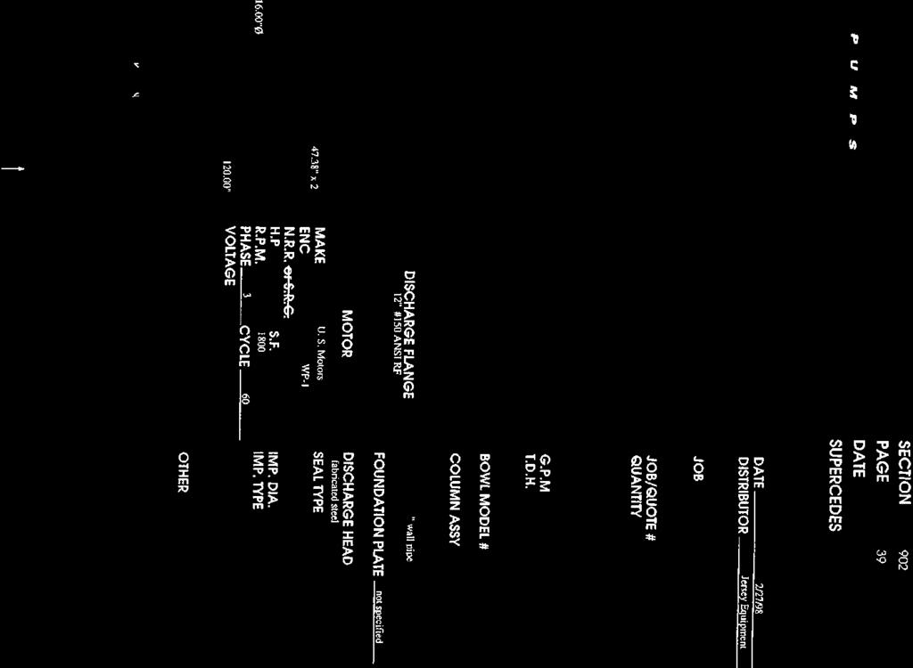
98

99 Surveyor Pump Station: Pump Curve 1 January 14, 2016

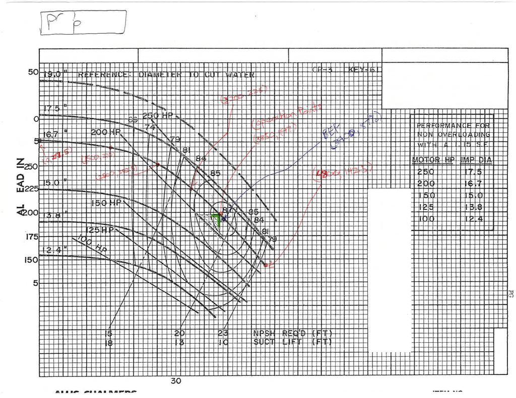
100

101 Surveyor Pump Station: Pump Curves 2 & 3 January 14, 2016

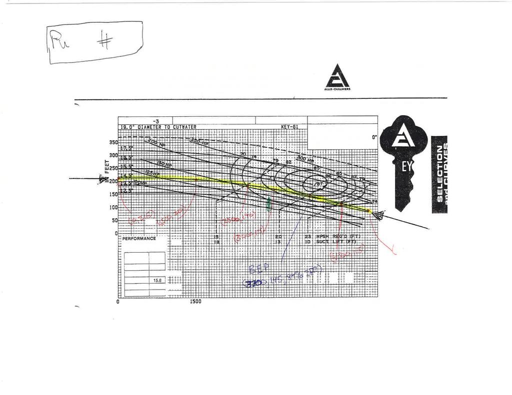
102

103 Appendix D Detailed Fire Flow Test Request Package January 14, 2016 APPENDIX D

104

105

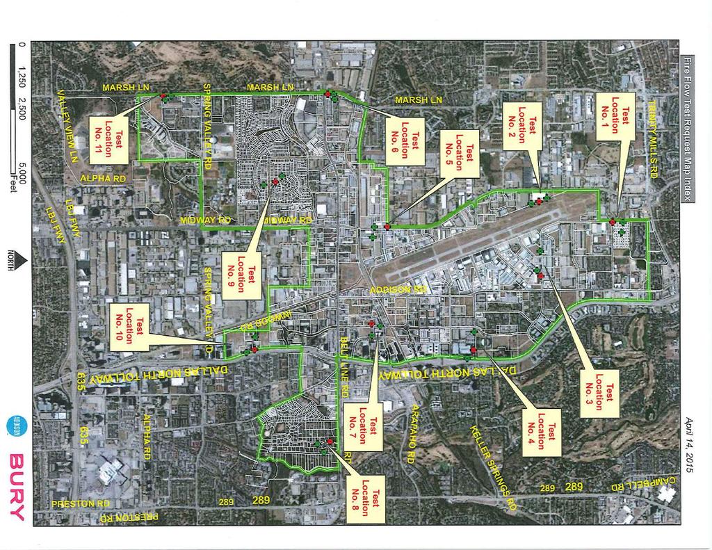
106

107

108

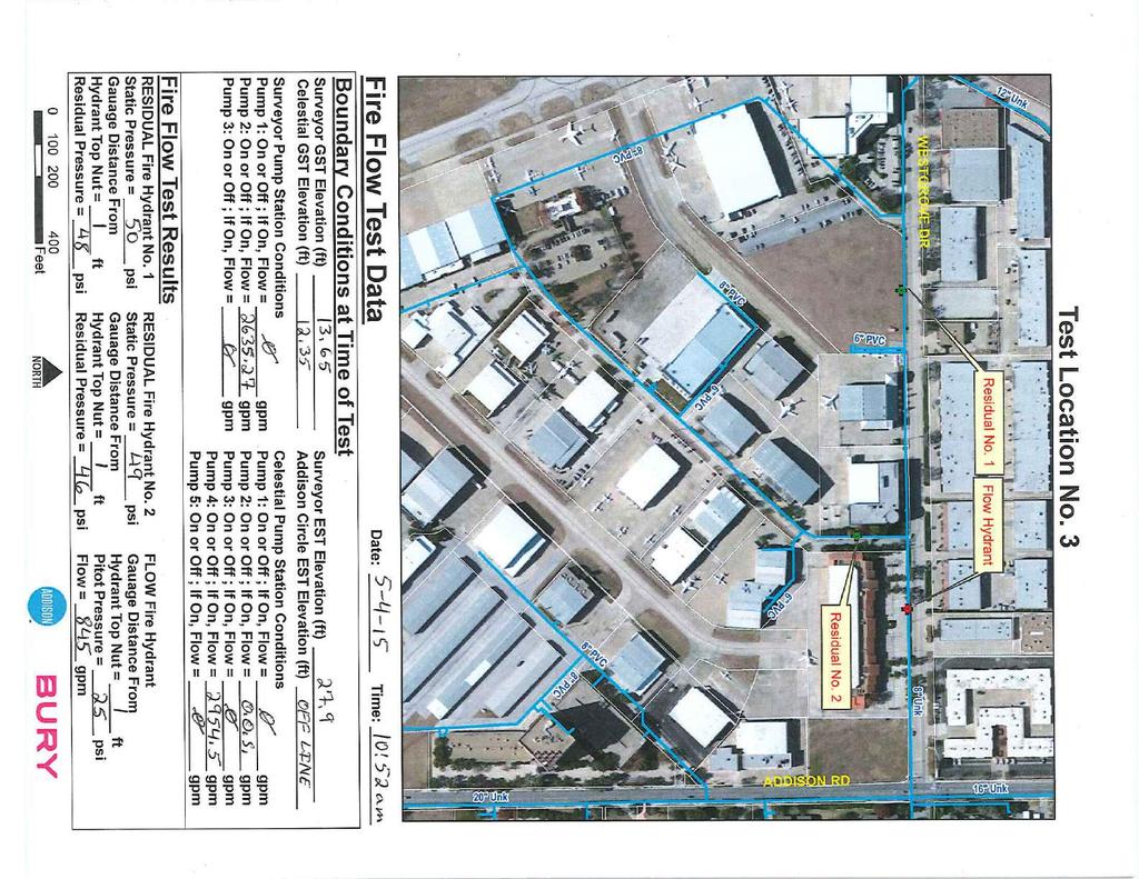
109

110

111

112

113

114

115