Carbon Monitoring System Flux Pilot Project

Transcription

1 Carbon Monitoring System Flux Pilot Project NASA CMS team: Kevin Bowman, Junjie Liu, Meemong Lee, Dimitris Menemenlis, Holger Brix, Joshua Fisher Jet Propulsion Laboratory, California Institute of Technology Joint Institute for Regional Earth System Science and Technology, University of California, Los Angeles Steven Pawson, Lesley Ott, James Collatz, Watson Gregg, Zhengxin Zhu, Randy Kawa, Cecile Rousseaux NASA Goddard Space Flight Center Chris Hill, Mick Follows, Stephanie Dutkiewicz MIT Kevin Guerney Arizona State University Gregg Marland, Eric Marland, Chris Badurek Appalachian State University Scott Denning Colorado State University Daven Henze, Nicholas Bousserez University of Colorado, Boulder Dylan Jones University of Toronto Ray Nassar Environment Canada California Institute of Technology. Government sponsorship acknowledged

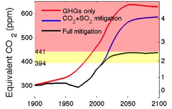
2 14 NATURE VOL497 2MAY2013 Ramanathan and Xu, PNAS (2010)

3 Multi-scale mitigation efforts California AB-32 Nature, Dec Independent efforts are being made to help mitigate climate change

4 A changing carbon cycle Science, 2008 Changes in the physical climate may undermine the ability of the natural carbon cycle to partially sequester atmospheric CO2 Saatchi et al, PNAS, 2013

5 Carbon Monitoring System Flux Pilot Project The objective of the NASA CMS Flux Project is to incorporate the full suite of NASA observational, modeling, and assimilation capabilities to attribute climate forcing to spatially resolved surface fluxes across the entire carbon cycle.

6 Bottom-up Satellite data Bottom-up assimilation/models GEOS-Chem CO2 transport model Land Surface data (fpar, EVI, etc) Land CASA/ CASA- GFED/ Sib4 GPP, Rh, BB x a,s a Meteorology GEOS-5 Top-down inverse model Ocean data (chlorophyll, salinity, etc) Ocean NOBM/E CCO2/D arwin ASE Fossil fuel emissions: FF GOSAT xco2 new satellite data GOSAT fluorescence Human FFDAS Top-down flux estimates and uncertainties Anthropogenic data (nightlights)

7 Spatial attribution of CO 2 Annual mean prior flux (gc/m 2 /day) Annual mean posterior flux (gc/m 2 /day) Post-prior (gc/m 2 /day) Zonal redistribution of carbon uptake in the Northern Hemisphere between Europe (stronger) and North America (weaker) Zonal redistribution in the tropics with reduced uptake in Africa but increased uptake in the Amazon India and China become net sinks. 7

8 Anthropogenic emissions and Biomass burning MOPITT V5 NIR/TIR, April 2010 Kar et al, ACP 2010 showed elevated, CO, AOD and ozone have been observed from space in the Eastern Indo-Gangetic Planes. Elevated CO 2 in Southeast Asia and Western China is broadly consistent with enhanced CO. Elevated CO 2 in Africa north of the ITCZ consistent with MODIS firecounts.

9 European sink and African biomass burning Europe and Western Russia are significant sinks

10 Conclusions and future directions The NASA Carbon Monitoring System is a critical link between surface fluxes and climate forcing. CMS flux pilot team has successfully integrated a carbon cycle modeling and attribution system constrained by anthropogenic, terrestrial, ocean, and atmospheric data. Preliminary results: Seasonality shifted forward Zonal shift in negative flux from West to East in the Northern Hemisphere. Zonal shift in negative flux from East to West in the Southern Hemisphere tropics and subtropics. Enhanced CO2 along the Eastern Indo-Gangetic Plane and throughout East Asia and China in the Northern Hemispheric Winter. Underestimate in biomass burning amplitude but consistent seasonality. Strong uptake in Europe and Western Russia Possibly due temporal aliasing of unobserved regions in the NH Winter and Fall. Several approaches to calculating formal uncertainties in progress (Bousserez, CU Boulder) More information at and

11 BACKUP

12 Impact of spatial sampling y-h(x a ) (prior flux) y-h(x ) (posterior flux) ppm Residual difference (obs-model) shows a strong meridional shift during NH summer. Tropical sampling driven by the ITCZ Large parts of the world are not observed Southern Hemisphere Northern Hemisphere during Winter and Fall Mean residual difference markedly reduced over the year. Pattern of differences largely the same Over correcting at mid-high latitudes in the NH during summer time;

13 Posterior uncertainty estimates Posterior uncertainties are calculated based upon a Monte Carlo method.

14 Attribution strategy CO2 accumulation ppm yr -1 Atmosphere (GOSAT): 2.36 ppm/yr Anthropogenic flux: GtC/yr Ocean flux: GtC/yr Inferred terrestrial flux: ~-2.48 GtC/yr Model: GEOS-Chem running on 5 x4 resolution with 47 vertical levels; Meteorology fields: GEOS-5 analysis Prior flux: CDIAC monthly fossil fuel emissions GFED 3 daily biomass burning ECCO2-Darwin ocean flux CASA-GFED 3 biosphere flux ACOS bias correction follows Wunch et al. (2011)

15 4D-var assimilation approach State vector Initial conditions q 0 q a Flux e 1 e 2 e 3 Both an initial condition and boundary condition problem Initial conditions solved through sliding window technique from Feng and Jones (UT) Monthly NEE estimated over a year window. Estimate of terrestrial flux only 4D-var x: monthly scale factor [S a ] ii = 50% based on CASA-GFED3 S n = Observational error from ACOS. No transport error or horizontal correlation error.

16 Posterior fit to GOSAT observations Annual global mean difference between GOSAT and model is less than 0.1 ppm (by construction). Springtime underestimate in prior model corrected by about 0.5 ppm in posterior model NH summertime overestimate is corrected by up to 2ppm in posterior model. SH correction of up to 1ppm in October. 16

17 Posterior flux estimate 2010 Prior flux (Black); Posterior flux (red and green) Posterior estimate redistributes the flux in space and time. The posterior flux increases carbon uptake over the NH mid-latitude and SH suptropics while reducing uptake over the tropics relative to the prior. Increased uptake in the first 6 months and reduced uptake in the last 6 months 17