Introducing the Granular Sludge Sequencing Tank

Transcription

1 BioWin Advantage Volume 7 - Number 2 - March 2018 Introducing the Granular Sludge Sequencing Tank Files : Case 1 1 d Two GSSTs.bwc Case 2 1 d Two GSSTs.bwc Case 3 - Aeration Controller.bcf Case 3A 1 d control Two GSSTs.bwc Case 3B 1 d control Two GSSTs.bwc Contents : Introduction... 2 Input Information in the GSST Setup... 5 Screen Output Simulating a GSST Plant Case 1: Low strength municipal influent Case 2: Higher strength municipal influent Case 3: BioWin Controller Approach Case 3A: Add post-anoxic period to certain cycles using BioWin Controller Case 3B: Improve nitrogen removal and optimize aeration using BioWin Controller.. 31 Conclusion References EnviroSim Associates Ltd McMaster Innovation Park 114A Longwood Road South Hamilton, Ontario L8P 0A1 Canada YouTube Facebook Twitter LinkedIn tel :: fax

2 Introduction This issue describes the Granular Sludge Sequencing Tank (GSST) element introduced in BioWin Version 5.3. The document covers several aspects: The basic requirements for setting up the GSST element (initial conditions, cycle times, etc.) and running dynamic simulations. [No steady state simulations with the sequencing unit]. Examples of simulating two GSSTs in parallel with an upstream buffer tank receiving municipal wastewater with a diurnal pattern. How to apply an irregular aeration pattern in one of the GSSTs using the BioWin Controller 2

3 In GSST operation there are four distinct phases, and in BioWin the sequence is as follows: The cycle starts at the beginning of the mixed phase. Typically, the reactor is full or nearly full at this point. During the mixed phase granular sludge and mixed liquor are well-mixed. The reactor may be continuously aerated during the mixed phase or may involve unaerated and aerated periods (based on DO setpoint or air flowrate). The settling phase commences when mixing stops. Granules immediately form a settled bed on the base of the reactor (with a void volume) and mixed liquor solids settle on top of the granular sludge bed. Typically waste activated sludge (WAS) is withdrawn from the bottom of the settled mixed liquor solids prior to commencing feed. We therefore anticipate a high concentration of WAS solids (and small volume). Granules are never removed directly during wasting, only bulk mixed liquor. However, there is turnover of granular mass via attachment and detachment from the granule surface. Influent feed typically commences well into the settling period. At this point the upper section of the reactor should be well-clarified liquid. Influent is distributed across the base of the reactor (into the granular sludge voidage) and flows in plug-flow mode up through the reactor. At the top level, liquid overflows into launders and is displaced as effluent. At the end of the settle/feed phase, prior to commencing the next cycle s mixed phase, there may be a small decant of clarified liquid near the top of the reactor to drop the liquid level below the launders. This prevents spillage of mixed reactor contents when the next cycle starts. The GSST modeling approach applies the full BioWin ASDM throughout the variable volume unit. Detailed physical-chemical modeling (ph, chemical precipitation, gas/liquid mass transfer, etc.) is included. BioWin s one-dimensional biofilm model is used to mimic the granular sludge; biofilm thickness is equivalent to granule radius. Settling of mixed liquor (non-granule) solids is based on a one-dimensional solids flux model. The bulk liquid above the bed of settled granules is divided into n equal-depth layers during settling. The GSST flowsheet element in BioWin is shown here. The granular sludge mass is represented by a biofilm with a calculated area and film thickness. The biofilm thickness is assumed to be equivalent to the average granule radius. The model does not predict new granule formation or consider a granule size distribution, but the diameter and composition of granules can change dynamically depending on substrate loading, as well as physical aspects such as solids impingement/erosion. 3

4 4

5 Input Information in the GSST Setup This section describes the rationale behind some of the default settings within the GSST element when it is first placed on the drawing board. It is important to note that these are not intended to serve as strict design guidelines, but rather, as reasonable starting points. Dimensions tab A GSST typically is 16 to 30 feet (5 to 10 m) deep. When the GSST element is placed onto the drawing board, the default depth is 6 m. Granules tab The user specifies initial estimates for the granule diameter (D), the granular sludge settled volume fraction (FG), and a voidage fraction (E) for settled granules, as follows: Estimated granule diameter (D) [mm]: This sets the initial diameter of the granules at the beginning of a simulation started from seed conditions. The actual diameter is a simulated output and will change from the initial estimate over the duration of a simulation. Estimated granule settled volume fraction (FG): This sets the initial estimate of the reactor volume (Vt) occupied by granules when granules are settled on the bottom of the reactor; this includes the intergranular voidage. This value is applied at the beginning of a simulation from seed conditions. The actual settled volume is a simulated output and will change from the original estimate over the duration of a simulation. Voidage (of settled granules) (E): This sets the percentage of the granule settled volume occupied by voidage. Although the granule diameter and settled volume are simulated and may change over the course of a simulation, the voidage percent is assumed to remain constant over the duration of a simulation. 5

6 These user-defined parameters are used to calculate the base granular surface area (A) [in metric units]: The base granular surface area and the user-specified voidage fraction are held constant throughout a dynamic simulation. The GSST model dynamically calculates the granular diameter depending on a number of factors such as substrate loading, reactions within the granules, and solids exchange between the granules and the bulk liquid. The granular settled volume fraction of the reactor volume changes proportionally to the model-calculated granular diameter, according to the rearranged base granular surface area equation: 6

7 In the examples presented below, the specifications are: Vt = 10,000 m 3 ; D = 0.8 mm; FG = 16%; and E = 25%. This results in a base granular surface area of 3,000,000 m 2, and the granular surface area to tank volume ratio is 300 m 2 /m 3. Experience indicates that D may range from say 0.6 to 1.5 mm, and the voidage likely is in the range of 20 to 28%. In addition, it appears that the granular surface area to tank volume ratio [A/Vt] should be in the range of 300 to 500 m 2 /m 3. If the user selects a target diameter (D) and a voidage fraction (E), an initial estimate of the FG value could be obtained from: For a desired granule diameter of 0.8 mm and a surface area to tank volume of 300 m 2 /m 3 at a voidage of 25%, the FG fraction would be 0.16 (16%). Operation tab The major operational settings for the GSST is the cycle information. The user specifies the cycle length, when settling starts, and when the decant starts. Default settings when a GSST element is added to the drawing board are shown below. 7

8 The user may specify the aeration settings in the GSST using a DO setpoint or air flow rate at a constant value or following a defined pattern. It is also possible to set up an irregular aeration pattern using BioWin Controller. This will be explained in an example later. The react/mix phase in the GSST element sets the maximum time span for aeration; BioWin shuts off aeration in the GSST during the settling period. Waste tab Typically thickened mixed liquor is removed from the GSST partway into the settling period, before the GSST is fed. Granules are never wasted from the GSST, only bulk mixed liquor. If wasting occurs during the settling period, it is removed from the bottom settled layer. Initial values tab 8

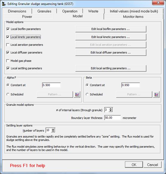
9 The user may specify the initial settings of the bulk mixed liquor concentrations and liquid holdup in the GSST element. Power options The user may enter power specifications for mechanical mixing in the GSST. Power can be specified on a power per unit volume basis or on a fixed basis at a constant value or in a pattern. Model tab When a GSST element is placed onto the drawing board, local biofilm, kinetic, diffuser and settling parameters are applied, as shown below. This is done to allow certain parameter values in the GSST to differ from BioWin s global defaults. The reasoning for adjusting these particular parameter values is outlined in the Help manual. 9

10 10

11 Screen Output Flyby panes Flyby panes below the BioWin configuration diagram report the following values for the GSST; note that the user is given an indication of what parameters are set locally by red text. Physical parameters (bottom left): Performance parameters (bottom right): 11

12 Simulating a GSST Plant All of the examples presented below are based on simulating two GSSTs in parallel with an upstream buffer tank receiving influent with a diurnal pattern. The first two cases consider treating either low strength or higher strength municipal raw influent. A third case shows how to apply an irregular aeration pattern in one of the GSSTs using BioWin Controller. Notes Pertaining to the General Setup: Oxygen modeling was applied throughout the simulation with a specified maximum air flow rate. The total SRT of each GSST is calculated based on the total mass in the GSST divided by the total mass rate wasted in both the Effluent and Wastage elements. The total SRT of GSST #1 and GSST #2 are plotted dynamically in the album. As a trick to smooth the calculated SRT [wasting is intermittent], a buffer tank has been added to each effluent and wastage pipe to mix each stream (labelled Mixed E and Mixed W ). The outflow from each Mixed E and Mixed W buffer tank is set at a constant flow rate. Once this file is simulated for 3 or 4 SRTs and allowed to reach quasi steady-state, the dynamic SRT in each GSST stabilizes to a relatively constant value (i.e. 20 days for the weak influent example and 27 days for the strong influent example). When changing any flow rate or pattern around each GSST (i.e. wastage, decant, influent and overflow), the outflow rate from each Mixed E and Mixed W buffer tank should be recalculated and adjusted. The tank volume and initial liquid hold-up may also need to be adjusted in each Mixed E and Mixed W buffer tank. The municipal influent has a typical wastewater fractionation. In these examples the average influent flow rate is 32,000 m 3 /d. The influent flow and loading follow a diurnal pattern. Buffer Tank and Cycle Offset A buffer tank is used to store influent and regulate the flow of influent to the two parallel GSSTs. Flow is pumped out of the buffer tank at a rate of 64,000 m 3 /d for 3 hours from 2:45 until 5:45 during each 6-hour cycle. For 1.5 hours of the 3 hours, outflow is directed to GSST #2, and then to GSST #1 for the remaining 1.5 hours. Over the 4 cycles in the day there is outflow from the buffer tank at a constant rate of 64,000 m 3 /d for a total of 12 hours. This is equivalent to the average influent flow rate of 32,000 m 3 /d to the buffer tank. A flow splitter downstream of the buffer tank routes the flow to GSST #2 from 2:45 until 4:15 and then to GSST #1 from 4:15 until 5:45 during each 6-hour cycle. The volume of influent fed to each GSST per cycle is calculated as follows: 12

13 Because the GSST is always operated full or nearly full (i.e. close to 10,000 m 3 ), it overflows shortly after feeding commences. The volume exchange ratio is defined as the volume fed per cycle divided by the liquid volume in the reactor. The volume exchange ratio is therefore approximately 40% in this example. The cycle settings for GSST #1 and GSST #2 are shown in the figure below. Each GSST has a cycle length of 6 hours. GSST #1 is the reference module and therefore has no cycle offset. GSST #2 operates with the same cycle as #1, but there is an offset relative to #1. We can think of the offset as how far we are into the #2 cycle when the #1 cycle starts. In this case, the cycle offset is 1.5 hours. Therefore, the simulation will start at time 0:00 in GSST #1 and at time 1:30 in GSST #2. Due to the cycle offset of 1.5 hours in this example, at least one of the GSSTs will end partway through a cycle when running a dynamic simulation of any given duration. Note: In this cycle set up, an offset of 1.5 hours is used, and this allows the outflow from the buffer tank to operate for 3 hours, four times per day. During each 3 hour period each GSST receives inflow for 1.5 hours. An alternative would be to have an offset of 3 hours, with eight 1.5 hour outflows from the buffer tank, and 4 going to each GSST. In that situation it may be possible to reduce the volume of the buffer tank slightly. Cycle Operation The detailed operational schedule of each GSST in the examples is shown below. 13

14 Thickened mixed liquor is removed from the bottom settling layer of the GSST partway into the settling period, just before the GSST starts feed. Granules are never wasted from the GSST, only bulk mixed liquor. Influent is fed to each GSST from 255 min (4:15) until 345 min (5:45) during each 6-hour cycle. As mentioned above, GSST #2 has a cycle offset of 1.5 hours to allow the GSSTs to be fed sequentially. Immediately after the feeding period in the GSST, a small decant is applied to drop the liquid level in the GSST prior to commencing the mix/react phase. Aeration The aeration cycle in each GSST is set up as follows: Unaerated for the first 30 minutes to promote denitrification using influent carbon fed at the end of the previous cycle. Aerated at a DO setpoint of 2.0 mg/l until settling begins at 3:30 and aeration is automatically shut off. Oxygen modelling is always applied and the maximum air flow rate is specified at 18,500 m 3 /h in the Case 1 weak influent example and 30,000 m 3 /h in the Case 2 strong influent example. (In order to determine a suitable maximum air flow rate, the model was first simulated from seed with oxygen modeling but without a maximum air flow rate constraint). The figures below show the results for the Case 1 weak influent scenario. The top plot shows the DO concentration that would be measured by a DO probe placed just below the liquid surface in the GSST. The bottom plot shows the air flow rate in each GSST. The Case 2 timeseries plots of DO concentration and air flow rate in the GSSTs are very similar to those presented below for Case 1 excepting that the maximum air flow rate is 30,000 m 3 /h. In GSST#1 the air is switched on at 0:30 AM and switched off when settling commences at 3:30 AM. BioWin adjusts the airflow rate to achieve the specified DO set point of 2 mg/l during this period, while remaining within the specified maximum air flow rate of 18,500 m 3 /h. When settling commences at 3:30 AM, the solids quickly settle out of the top liquid layer. The OUR in this top layer rapidly declines and hence substantial DO remains here. Feeding commences at 4:15 which displaces oxygenated liquid over the top of the tank. The DO concentration just below the liquid surface subsequently decreases as less oxygenated liquid is displaced upward. At 6 AM settling ends and mixing commences. The granules are mixed with the settled bulk mixed liquor. Any remaining DO is rapidly consumed during the pre-anoxic period. 14

15 Influent The influent flow and TCOD, TKN and TP concentrations follow a diurnal pattern. The table below shows the average influent flow and flow-weighted average influent concentrations of TCOD, TKN and TP applied in Case 1 and Case 2. The values of the other influent parameters (ph, Alkalinity, ISS, etc.) were held at the same constant values throughout the day in both cases. Initializing the simulations 15

16 In all the examples the parallel GSST plant was dynamically simulated from seed values for an extended period (e.g. 4 SRTs) until a quasi-steady-state was reached. The plot below shows how the total solids mass each GSST achieves a stable condition. When simulating from seed values, a data interval of 1 hour was applied to speed up simulations. The data interval was then decreased to 1 minute and the model was simulated from the current values for one day. The files were then saved at that condition. The short data interval improves the resolution of the time-series plots so that they show every scheduled change in influent load, wastage flow rate, aeration setting, etc. The data interval can be changed back to 1 hour before simulating this file for a longer period of time to improve the simulation speed. All of the four accompanying BioWin files were generated by simulating for an extended period to attain the quasi-steady-state, and then simulating for one day from current values. The results shown later cover longer periods, but the files were saved with only one day of results to reduce file sizes for downloading. 16

17 Case 1: Low strength municipal influent The section below shows results for Case 1. The flow-weighted average influent TCOD, TKN and TP concentrations were 400 mgcod/l, 40 mgn/l and 4 mgp/l, respectively. The results for 5 days of operation were generated by opening the accompanying BioWin file Case 1 1 d Two GSSTs.bwc and simulating from project start date for 5 days from current values. Effluent Concentrations The figures below show the effluent ammonia and NOX concentrations from each GSST. The 24- hour flow weighted concentrations are 0.1 mgn/l and 7.2 mgn/l, respectively. The 24-hour flow weighted composite effluent TP and spo4-p concentrations from each GSST are 0.2 mgp/l and 0.1 mgp/l, respectively, as shown in the figure below. 17

18 The effluent TSS concentration from each GSST was 5.4 mg/l, as shown in the figure below. The BioWin album of Case 1 1 d Two GSSTs.bwc contains numerous other plots to further assess the performance of the Case 1 scenario for this parallel GSST plant. 18

19 Case 2: Higher strength municipal influent The section below shows results for Case 2. The flow-weighted average influent TCOD, TKN and TP concentrations were 600 mgcod/l, 60 mgn/l and 6 mgp/l, respectively. The results for 5 days of operation were generated by opening the accompanying BioWin file Case 2 1 d Two GSSTs.bwc and simulating from project start date for 5 days from current values. Effluent Concentrations The figures below show the effluent ammonia and NOX concentrations from each GSST. The 24- hour flow weighted concentrations are 0.2 mgn/l and 8.4 mgn/l, respectively. The 24-hour flow weighted composite effluent TP and spo4-p concentrations from each GSST are 0.2 mgp/l and 0.1 mgp/l, respectively, as shown in the figure below. 19

20 The effluent TSS concentration from each GSST was 5.5 mg/l, as shown in the figure below. The BioWin album of Case 2 1 d Two GSSTs.bwc contains numerous other plots to further assess the performance of the Case 2 scenario for this parallel GSST plant. The results presented for Case 1 and Case 2 demonstrate the capacity of the parallel GSST plant to achieve a good level of biological nitrogen and phosphorous removal and low effluent suspended solids. The plant performs very well even when treating the higher strength influent. However, can nitrogen removal performance be further improved? This is evaluated in Case 3. 20

21 Case 3: BioWin Controller Approach The aim of Case 3 is to improve nitrogen removal in the Case 1 weak influent scenario. We investigated two approaches for increasing the anoxic period in mixing cycles to improve denitrification while at the same time minimizing the impact on nitrification. 21

22 Case 3A: Add post-anoxic period to certain cycles using BioWin Controller We started with the Case 1 weak influent case. We wished to modify the aeration pattern in GSST#1 to include a post-anoxic period in certain cycles during the day. [The aeration schedule was kept the same in GSST #2 (as specified on the operation tab) for comparison purposes]. The objective was to add a post-anoxic period to cycles in GSST #1 following feed events with relatively lower ammonia load. The plant influent has a diurnal flow and loading pattern and the influent buffer tank regulates the flow to the GSSTs. The TKN mass rate to each GSST is shown in the plot below for the Case 1 weak influent scenario. The cycles in GSST#1 are also indicated on the plot. The TKN and ammonia load entering GSST#1 is higher during cycles 2 and 3 compared to cycles 1 and 4 as a consequence of the influent diurnal loading pattern. GSST#1 is fed at the end of each 6-hour cycle, i.e. from 4:15 until 5:45 as shown by the red line in the plot above. Shortly after this feeding period, the mixing period of the next cycle commences. The desired approach for achieving improved N removal was to adjust aerated versus anoxic periods in certain cycles. For example, with a lower ammonia load in cycle 1, presumably the aerated period in cycle 2 can be reduced while still achieving complete nitrification. Specifically, we wished to evaluate the following changes to increase the amount of NOX removed by denitrification: Adding a 30-minute unaerated (post-anoxic) period by shortening the aerated period in cycle 2. This was added over the last 30 minutes of the mixing period from 3:00 until 3:30 in the cycle (or 09:00 to 09:30 in the 24-hour period shown in the plot above). 22

23 Similarly, an anoxic period was added in cycle 1 in the same way because this cycle also follows a relatively low influent ammonia load in cycle 4. Because cycles 2 and 3 treat relatively higher influent ammonia loads, the aeration periods in these cycles were not shortened. It is not possible to specify different aeration patterns from one cycle to the next in the GSST element. However, this can be achieved using an approach with the BioWin Controller. The BioWin Controller was used to specify an alternative aeration pattern on a 1-day cycle, to override the 6-hour repeated aeration pattern in the operation tab of GSST#1. We first created a table of the desired DO set points and relevant events in the four cycles in GSST#1 during a 24-hour period, as shown below. BioWin always shuts off aeration during the settling period in the GSST, regardless of the aeration control strategy applied using BioWin Controller. Therefore, it is not necessary to schedule the aeration shut off during the settling periods. The 1-day aeration schedule in GSST #1 therefore can be simplified as shown in the following table. 23

24 The BioWin Controller cannot be used to set up this schedule directly. The trick to get around the limitation is to input the schedule via a dummy element which includes a time schedule. The simplest approach is to use a COD Influent element. In this example an influent element [DO Schedule (in Flow)] is connected to an effluent element [DO Schedule (exit)] as shown in the flow sheet figure below. In the DO Schedule (in Flow) element the time-varying DO set point is specified in the Flow column. The time and flow values in this influent itinerary match the respective time and DO set point values shown in the previous table. As will be explained further below, the BW Controller file reads this data and uses this to control the DO in GSST#1 according to the specified pattern. The cycle time of the DO Schedule (in Flow) influent itinerary was specified 24

25 as 1 day. The default concentration for all the other influent parameters (COD, TKN, TP, etc.) are ignored. BioWin Controller Setup Three controllers are set up in the Controller list: DO Controller, DO Controller Setpoint, and DO Controller UBound. The DO Controller is a PID controller that adjusts the air flow rate in GSST #1 (Manipulated variable) with the objective of maintaining the DO in GSST #1 (Measured variable) at a set point. The setup of the DO Controller is shown in the figure below. The setpoint initially is specified as 0 mg/l. 25

26 Essentially all the control work is performed by the DO Controller. However, the two additional controllers listed are there because: In the DO Schedule (in Flow) element the desired setpoint values/changes are specified in the Flow column with units of m 3 /d. The function of the DO Controller Setpoint is to convert the flow units to DO units essentially by multiplying by a factor of 1. When the GSST is aerated the DO Controller UBound controller imposes the maximum air flow limit. The DO Controller Setpoint is a ratio controller that adjusts the setpoint of the DO Controller (Manipulated variable) in a fixed proportion to the value in the Flow column in the DO Schedule (in Flow) influent element. As shown in the figure below, the manipulated variable is equal to the specified ratio multiplied by the measured variable. The ratio is specified as 1 [mg/l]/[m 3 /d]. Therefore, a flowrate of 1 m 3 /d in the DO Schedule (in Flow) influent element is equivalent to a DO setpoint of 1 mgo2/l. 26

27 The third controller, DO Controller UBound, is a user-defined controller that adjusts the upper bound of DO Controller (manipulated variable) based on the Flow in DO Schedule (in Flow) influent element. A controller formula was used to set the upper bound of the air flow rate to 18,500 m 3 /h for the weak influent scenario when the Flow (i.e. DO setpoint) in DO Schedule (in Flow) was greater than 0.01 (i.e. when the GSST is aerated). Otherwise the upper bound of the air flow rate was set to 0 m 3 /h. The DO Controller UBound set up is shown in the figure below. 27

28 Further details on BioWin Controller are found in the BioWin Controller Help manual. The BioWin Controller strategy was applied and the simulation was continued from current values for 10 days. The figure below shows the DO concentration and air flow rate in each GSST over the last day of simulation with BioWin Controller manipulating the aeration in GSST#1. An analysis of these plots shows that the BioWin Controller strategy is working as intended. The first and second cycles in GSST#1 have 30 minute pre- and post-anoxic periods at the beginning and end of the mixing phase. When aeration is shut off at the beginning of the post-anoxic period (3:00 into the cycle) in GSST#1, the DO rapidly drops to zero because the granules and bulk mixed liquor are mixed and the OUR is high. The second and third cycles in GSST#1 only have a 30-minute pre-anoxic period, as do all of the cycles in GSST #2. When settling commences at 3:30 PM in cycle 3 in GSST#1, the solids quickly settle out of the top liquid layer. The OUR in this top layer rapidly declines and hence substantial DO remains here. 28

29 Effluent Concentrations The figures below show key effluent concentrations for the Case 3A scenario. The time axis shows 15 days of simulation. The Case 1 (low strength influent) scenario was simulated for 5 days at quasi-steady-state without BioWin Controller. The BioWin Controller file was then opened and the simulation was continued for 10 days to apply a 30-minute post-anoxic period to certain mixing cycles in GSST#1. The accompanying BioWin file Case 3A 1 d control Two GSSTs.bwc was simulated from project start date for 1 day from current values (with BioWin Controller) to minimize the file size. (The current values were at the end of the 10 days of simulation with BioWin Controller). After the irregular aeration pattern was applied in GSST#1, the 24-hour flow weighted composite effluent ammonia and NOX concentrations levelled off at 0.3 mgn/l and 5.9 mgn/l, respectively. Comparing these values to the respective values of 0.1 mgn/l and 7.2 mgn/l in GSST#2 shows that the post-anoxic periods applied in certain cycles in GSST#1 improved denitrification with minimal impact on nitrification. 29

30 After the irregular aeration pattern was applied in GSST#1, the 24-hour flow weighted composite effluent TP and spo4-p concentrations remained essentially the same as those from GSST#2, as shown in the figure below. In summary, the nitrogen removal in GSST#1 was improved by adding a post-anoxic period to certain mixing cycles that treat lower influent ammonia loads. Let s investigate whether we can further improve nitrogen removal and optimize aeration. 30

31 Case 3B: Improve nitrogen removal and optimize aeration using BioWin Controller The aim of Case 3B is to further improve nitrogen removal and reduce aeration requirements using BioWin Controller. We used the same BioWin Controller file as in Case 3A. However, we made adjustments to the irregular aeration pattern encoded in the DO Schedule (in Flow) influent element. In Case 3A, a 30-minute post-anoxic period was added to certain mixing cycles treating lower influent ammonia loads. In Case 3B we applied a post-anoxic period in every mixing cycle that was scheduled to commence when the ammonia concentration reached a low value close to zero (i.e. when nitrification is complete). We started with the Case 1 weak influent file at quasi-steady-state conditions. The figure below shows the ammonia concentration in GSST#1 over 24 hours before BioWin Controller was applied. The aeration pattern follows that specified in the operation tab (i.e. 30-minute pre-anoxic followed by aeration until settling beings at 3:30 into each cycle). The mixing period in cycles 1, 2, 3 and 4 are also indicated on the figure. Instead of applying a 30-minute postanoxic period in cycles 1 and 2 as was done in Case 3A, we added a post-anoxic period to every cycle that commenced when the ammonia concentration essentially reached zero, and nitrification was complete. The ammonia in the tank reached zero at approximately 2:30 AM (cycle 1), 8:15 AM (cycle 2), 2:45 PM (cycle 3) and 9:00 pm (cycle 4), as shown in the figure below. Similar to Case 3A, we set up an influent element [DO Schedule (in Flow)] connected to an effluent element [DO Schedule (exit)]. We encoded a revised irregular aeration pattern in the DO Schedule (in Flow) influent element, as shown in the figure below. As was explained previously in Case 3A, the BioWin Controller file reads the time and flow values in the influent itinerary, converts flow into DO concentration and attempts to control the DO in GSST#1 at the specified setpoint. The time and flow values in the influent itinerary below were specified to allow a 30-minute pre-anoxic period at the beginning of each mixing phase and a post-anoxic period at the end of each mixing phase. The post-anoxic period was scheduled to commence when the ammonia was reduced to near zero. 31

32 We started with the Case 1 example that had been simulated for 5 days at quasi-steady-state without BioWin Controller. The BioWin Controller file was then opened and the simulation was continued from current values for 30 days. The Controller file applied the revised irregular aeration pattern to GSST#1. The aeration schedule was kept the same in GSST #2 (as specified on the operation tab) for comparison purposes. The figure below shows the DO concentration and air flow rate in each GSST over the last day of simulation with BioWin Controller manipulating the aeration in GSST#1. An analysis of these plots shows that the BioWin Controller strategy is working as intended. The post-anoxic periods in GSST#1 begin at 2:30 AM (cycle 1), 8:15 AM (cycle 2), 2:45 PM (cycle 3) and 9:00 pm (cycle 4), as scheduled. By comparison, GSST#2 does not have post-anoxic periods and so DO remains in the upper layers of the settled bulk mixed liquor until mixing commences. When aeration begins 30 minutes into the mixing period in each cycle, BioWin Controller adjusts the air flow rate to achieve the target DO set point of 2 mg/l. Because there is substantially less aeration in GSST#1 compared to GSST#2, the air flow remains at the maximum value in GSST#1 much longer than in GSST#2. As a result, the DO in GSST#1 dips slightly below the 2 mg/l set point for a portion of the aerated period. 32

33 Effluent Concentrations The figures below show key effluent concentrations for the Case 3B scenario. The time axis shows 35 days of simulation. The Case 1 (low strength influent) scenario was simulated for 5 days at quasi-steady-state without BioWin Controller. The BioWin Controller file was then opened and the simulation was continued for 30 days to apply irregular post-anoxic periods in GSST#1. The accompanying BioWin file Case 3B 1 d control Two GSSTs.bwc was simulated from project start date for 1 day from current values (with BioWin Controller) to minimize the file size. (The current values were at the end of the 30 days of simulation with BioWin Controller). After simulating for 30 days with the irregular aeration pattern applied in GSST#1, the 24-hour flow weighted composite effluent ammonia and NOX concentrations changed to 0.7 mgn/l and 1.6 mgn/l, respectively. By comparison, in Case 3A the 24-hour flow weighted composite effluent ammonia and NOX concentrations in GSST#1 levelled off at 0.3 mgn/l and 5.9 mgn/l, respectively. Therefore the optimized aeration strategy applied in Case 3B improved nitrogen removal although there was some loss of nitrification. 33

34 After simulating for 30 days with BioWin Controller, the 24-hour flow weighted composite effluent TP and spo4-p concentrations increased to 0.7 and 0.6 mgp/l, as shown in the figure below. However, these concentrations are still increasing and have not yet levelled off. The shortened aeration periods have decreased the amount of phosphorous that can be taken up by PAOs and removed through sludge wasting. In summary, the nitrogen removal was improved further in Case 3B compared to Case 3A. This improvement was made by adding a post-anoxic period to each mixing cycle that was scheduled to commence when the ammonia reached zero. An added benefit of increasing the unaerated period in each cycle is a reduction in the total aeration requirement for the plant. At 34

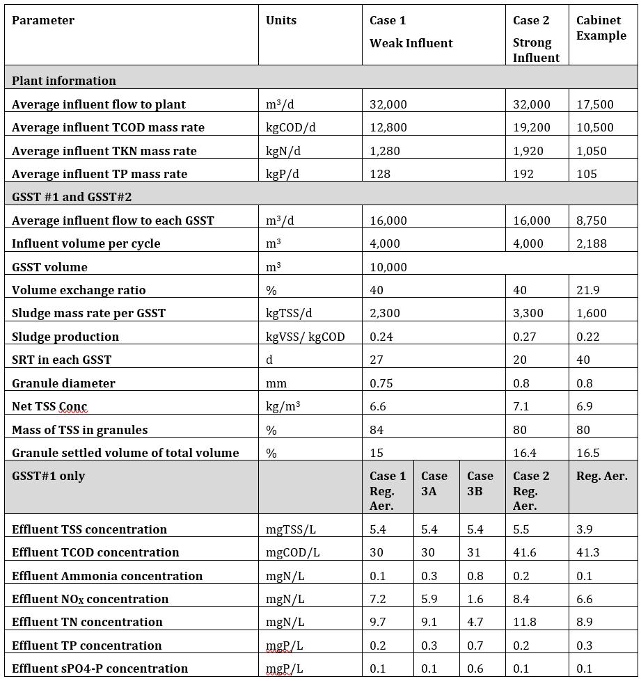
35 the same time, however, this change resulted in some loss of nitrification and biological phosphorous removal. Performance Summary for Cases 1, 2 and 3 A plant comprised of two GSSTs in parallel with an upstream buffer tank was simulated. A diurnal pattern was applied to the plant influent. The performance of the plant in treating low strength (Case 1) or higher strength (Case 2) municipal raw influent was assessed. Finally, BioWin Controller was used to apply an irregular aeration pattern in one of the GSSTs for the weak strength influent scenario to improve nitrogen removal (Cases 3A and 3B). The configuration of the plant presented in this document is similar to the BioWin Cabinet file Two GSSTs- diurnal effluent mix.bwc. In the table below, we compare the performance of this cabinet file with Cases 1, 2, 3A and 3B. The operational cycles in the GSSTs in the cabinet file are the same as in Cases 1, 2 and 3. The plant influent in the cabinet example has a diurnal pattern; however the average flow is lower than in Cases 1, 2 and 3. The GSST volume exchange ratio is also lower in the cabinet file compared to Cases 1, 2 and 3. The cabinet file has a lower sludge wasting mass rate and hence a longer SRT compared to Cases 1, 2 and 3. The calculated granule diameter, net TSS concentration in the GSST, mass of TSS in granules and granule settled volume are similar among the cabinet file and Cases 1, 2 and 3. A few things to note regarding this table: The specified values on the Granules tab of both GSSTs in every example were as follows: o Estimated granule diameter = 0.8 mm o Estimated granule settled volume = 16% o Voidage (of settled granules) = 25% The granular surface area each GSSTs was therefore the same in every example (i.e. 3,000,000 m 2 ) The sludge production is calculated as follows: o VSSWAS 1 and VSSWAS 2 are the average VSS mass rates in the wastage from GSST #1 and GSST#2, respectively o TCODINF is the average TCOD mass rate entering the plant o TCODEFF 1 and TCODEFF 2 are the average COD mass rates in the effluent from GSST #1 and GSST#2, respectivel At the bottom of the table, effluent parameter concentrations are provided for GSST#1 only. These represent the 24-hour flow-weighted average concentrations from the quasi-steady-state model. For the weak influent scenario discussed in this document, three different aeration patterns were applied in GSST#1: 35

36 o o o Reg. Aer. is the regular aeration pattern specified in the operation tab of GSST#1 (i.e. 30 minutes pre-anoxic followed by aeration at a DO setpoint of 2 mg/l until settling begins at 3:30 into each cycle) Case 3A is the irregular aeration pattern applied using BioWin Controller. In this pattern, cycles 3 and 4 have a 30-minute pre-anoxic period and cycles 1 and 2 have 30 minute pre- and post-anoxic periods. Case 3B is the revised irregular aeration pattern applied using BioWin Controller. In this pattern, a 30-minute pre-anoxic period was applied in every cycle along with a post-anoxic period that commenced when the ammonia concentration reached zero. The cabinet example has a regular aeration pattern that consisted of a 30-minute unaerated (pre-anoxic) period followed by aeration at a DO setpoint of 1.5 mg/l until settling began at 3:30 into each cycle. BioWin Controller was not applied in the cabinet example. 36

37 37

38 Conclusion In this edition of the BioWin Advantage, we described the Granular Sludge Sequencing Tank (GSST) element introduced in BioWin Version 5.3. Several aspects were covered: The basic requirements for setting up the GSST element (initial conditions, cycle times, etc.) and running dynamic simulations. [No steady state simulations with the sequencing unit]. An approach to simulate two GSSTs in parallel with an upstream buffer tank receiving municipal wastewater with a diurnal pattern. The performance of this plant was evaluated in treating low strength or higher strength influent. How to apply an irregular aeration pattern in one of the GSSTs using the BioWin Controller. Further details on the GSST element are found in the BioWin Help manual under: Building Configurations > Element Descriptions > Granular Sludge Sequencing Tank Model Reference > Modeling Granular Sludge Sequencing Tanks The BioWin cabinet folder also contains four example GSST plant models with detailed notes. We trust that you found this technical topic both interesting and informative. Please feel free to contact us at support@envirosim.com (Subject: The BioWin Advantage) with your comments on this article or suggestions for future articles. Thank you, and good modeling. From the EnviroSim Team References Pronk, M., de Kreuk, M.K., de Bruin, B., Kamminga, P., Kleerebezem, R. and M.C.M van Loosdrecht. (2015), Full scale performance of the aerobic granular sludge process for sewage treatment. Wat. Res., 84, EnviroSim (2018). BioWin User Manual, Model Description. Reichert, P. and Wanner, O. (1997). Movement of Solids in Biofilms: Significance of Liquid Phase Transport. Wat. Sci. Tech. 36 (1), Wanner, O. and Reichert, P. (1996) Mathematical Modeling of Mixed-Culture Biofilms. Biotechnology and Bioengineering 49,