An environmental assessment system for environmental technologies

Transcription

1 Downloaded from orbit.dtu.dk on: Nov 18, 2018 An environmental assessment system for environmental technologies Clavreul, Julie; Baumeister, Hubert; Christensen, Thomas Højlund; Damgaard, Anders Published in: Environmental Modelling & Software Link to article, DOI: /j.envsoft Publication date: 2014 Document Version Peer reviewed version Link back to DTU Orbit Citation (APA): Clavreul, J., Baumeister, H., Christensen, T. H., & Damgaard, A. (2014). An environmental assessment system for environmental technologies. Environmental Modelling & Software, 60, DOI: /j.envsoft General rights Copyright and moral rights for the publications made accessible in the public portal are retained by the authors and/or other copyright owners and it is a condition of accessing publications that users recognise and abide by the legal requirements associated with these rights. Users may download and print one copy of any publication from the public portal for the purpose of private study or research. You may not further distribute the material or use it for any profit-making activity or commercial gain You may freely distribute the URL identifying the publication in the public portal If you believe that this document breaches copyright please contact us providing details, and we will remove access to the work immediately and investigate your claim.

2 Accepted for publication in Environmental Modelling and Software Supplementary information EASETECH an Environmental Assessment System for Environmental TECHnologies Julie Clavreul 1, Hubert Baumeister 2, Thomas H Christensen 1, Anders Damgaard* 1 1 Technical University of Denmark, Department of Environmental Engineering, Building 113, DK-2800 Kongens Lyngby, Denmark 2 Technical University of Denmark, Department of Informatics and Mathematical Modelling, Building 303B, DK-2800 Kongens Lyngby, Denmark * Corresponding author Phone: Fax: adam@env.dtu.dk NOTE: this is the author s version of a work that was accepted for publication in Environmental Modelling and Software journal. Changes resulting from the publishing process, such as peer review, editing, corrections, structural formatting, and other quality control mechanisms may not be reflected in this document. Minor changes may have been made to this manuscript since it was accepted for publication. A definitive version is published in Environmental Modelling and Software, vol 60, pp 18-30, doi: /j.envsoft SI - 1

3 TABLE OF CONTENTS Part I: Example of testing of the conceptual model... 4 Part II: Screenshots... 5 Part III: Documentation of calculations Material composition calculations Material generation Energy generation Material generation manual Basic Substance transfer per fraction Substance transfer default Mass transfer to outputs Change of energy content No output Water content Addition of substances Emissions to the environment Landfill gas generation Mass transfer over years Leachate generation Anaerobic digestion Use-on-land LCA calculations in all processes: process-specific emissions and external processes An external process with only process-specific emissions: test An external process with process-specific emissions and one external process: test An external process with process-specific emissions and an external process that uses another external process: test A material process uses this external process Normalised and weighted impacts Particular case: Material generation Particular case: Energy generation Input-specific emissions in four material processes Substance transfer per fraction Substance transfer default Use on land (UOL) SI - 2

4 3.4 Emissions to the environment Part IV: Case study Scenario construction and data input Incineration scenario Anaerobic digestion (AD) scenario LCIA methods used Uncertainty propagation The table of parameters Material generation Material composition calculation LCI data in material process Calculation of the characterised impact References SI - 3

5 PART I: EXAMPLE OF TESTING OF THE CONCEPTUAL MODEL The testing of the conceptual model was performed using the FitNesse Wiki, an automated testing tool which uses the Framework for Integrated Tests (Fit) to evaluate user stories in the context of the developed conceptual model. Figure S1 presents an example of such a Wiki page testing the correct computation of life cycle inventories (LCI). This user story is one of the first ones that were implemented. It consists of 3 input tables and of one result table. The objective is to enter input values and check if the conceptual model gives the expected result in the last table. Note that the text outside of tables is only comments and is never evaluated. In the 1 st table, a waste process is defined that uses 2 MJ/kg of electricity per kg of wet weight of the input waste. This electricity is supplied by an external process called 1 MJ Electricity production (DK). The 2 nd table describes the elementary flows induced by the external process 1 MJ Electricity production (DK) : producing 1 MJ of electricity will emit 20 kg CO 2 into the air. The 3 rd table describes the waste input: here the waste has a wet weight of 2 kg. Finally the last table computes the LCI of the process. The green color shows that the result is the one we expected: the emission of 80 kg of CO 2 into the air. This simple example illustrates how basic calculations can be tested in the FitNesse Wiki. Figure S1: Example of a FitNesse Wiki page testing the conceptual model SI - 4

6 PART II: SCREENSHOTS All numbers refer to the general overview of the interface in Figure 5 of the article. Material transfer tab (2a): Process exchanges tab (2b): SI - 5

7 Documentation tab (2c): LCI tab (2d): SI - 6

8 Characterised impacts tab, per substance and per process views (2e): SI - 7

9 Normalised impacts tab, per substance and per process views (2f): SI - 8

10 Weighted impacts tab, per substance and per process views (2g): SI - 9

11 Composition tab (2h): Material fractions catalogue (4a): SI - 10

12 Elementary exchanges catalogue (4b): Impact categories catalogue (4c): SI - 11

13 Methods catalogue (4d): Interfaces catalogue (4e): SI - 12

14 Constants catalogue (4f): Material properties catalogue (4g): SI - 13

15 PART III: DOCUMENTATION OF CALCULATIONS This document was used to communicate with the development team and explain how calculations should be implemented. It uses simple words and lots of examples to illustrate the calculations happening in each template process. In a first section, the different calculations of output flow compositions are presented. The second section describes the general LCA calculations happening in all processes, related to data in the Process exchanges tab, i.e. external processes and process-specific emissions. The third section presents the inputspecific emissions calculated in 4 material processes whose Material transfer tab produces input-specific emissions. 1 Material composition calculations 1.1 Material generation In this process, the user defines a TotalAmount and the composition in terms of fractions (called percent here). Data about each fraction are taken in the library of material fractions. For each material fraction, water (kg) = water% (fraction)/100 *percent(fraction)/100 *TotalAmount (kg) vs(kg) = VS%(fraction) )/100 * percent(fraction) )/100 *TotalAmount(kg) ash(kg) = ash%(fraction) )/100 * percent(fraction) )/100 *TotalAmount(kg) energy (MJ) = energy%(fraction) * TS%(fraction)/100 *percent(fraction) )/100 *TotalAmount(kg) for all other material properties: materialproperty(kg) = materialproperty%(fraction) )/100 * TS%(fraction) )/100 * percent(fraction) )/100 *TotalAmount(kg) where e.g. ash% is the ash content of the fraction in the library of material fractions. Total wet weight and TS are calculated as usual, respectively as the sum of TS and water, and the sum of VS and ash. Figure S2 shows an example of material generation process. Figure S2: Material transfer of a Material generation process and catalogue of material fractions SI - 14

16 The output is (Figure S3): for fraction vegetable food waste : o water: 76.99/100 * 70/100 * 30 kg = kg o VS: 94.8/100*23/100*70/100*30 kg = kg o ash: 5.2/100 *23/100 *70/100 *30 kg =0.251 kg o energy: 18.3*23/100*70/100*30 kg = MJ o C bio: 47.5/100 *23/100 *70/100 *30 kg = kg o... for fraction office paper : o water: 8.75/100 * 30/100 * 30 kg = kg o VS: 79.3/100*91.3/100*30/100*30 kg = kg o ash: 20.7/100 *91.3/100 *30/100 *30 kg =1.701 kg o energy: 12.53*91.3/100*30/100*30 kg = MJ o C bio: 37.3/100 *91.3/100 *30/100 *30 kg = kg Figure S3: Material composition of the output of the Material generation process 1.2 Energy generation The user defines a TotalAmount and the composition in terms of fractions (called percent here). Data about each fraction is taken in the library of material fractions. For each material fraction, energy (MJ) = percent(fraction) /100 *TotalAmount(MJ) vs(kg) = VS%(fraction) )/100 * percent(fraction) )/100 *TotalAmount(MJ) /energy%(mj/kg) ash(kg) = ash%(fraction) )/100 * percent(fraction) )/100 *TotalAmount(MJ) /energy%(mj/kg) water (kg) = water%(fraction) / TS%(fraction) *percent(fraction)/100 *TotalAmount (MJ) /energy%(mj/kg) for all other material properties: materialproperty(kg) = materialproperty%(fraction) )/100 * percent(fraction) )/100 *TotalAmount(MJ) / energy%(mj/kg) where e.g. ash% is the ash content of the fraction in the library of material fractions. Total wet weight and TS are calculated as usual, respectively as the sum of TS and water, and the sum of VS and ash. Figure S4: Material transfer of a Material generation process and catalogue of material fractions SI - 15

17 Vegetable food waste is: Energy = 70/100 *30 MJ = 21 MJ TS = (70/100 *30 MJ) /18.3 MJ/kg = kg VS = (70/100 *30 MJ) /18.3 MJ/kg *94.8/100 = kg Ash = (70/100 *30 MJ) /18.3 MJ/kg *5.2/100 = kg Water = 76.99/23.01 *70/100*30 MJ /18.3 MJ/kg = kg Because the tickbox Mass is unticked for Office paper, this fraction has only: Energy = 30/100*30 MJ = 9 MJ Figure S5: Material composition of the output of the Material generation process 1.3 Material generation manual In this process, the user defines the number of fractions and the amounts of material properties directly. So the only thing to calculate is Total solids (TS) equal to VS+ash, and Total wet weight (TWW) equal to TS+waterContent. 1.4 Basic Output = input. 1.5 Substance transfer per fraction The number of outputs is determined by the user. The user can define the name of the output by right clicking on the column header in the table Material transfer. Each output has the same material fractions as the input (in terms of numbers and names). For each output, for each fraction, for each material property, outputnumber.fraction.property = input.fraction.property*tc(property, fraction, outputnumber)/100 where TC is a transfer coefficient input by the user in the table of Material transfer in an output column, in a material fraction line. If the fraction doesn t exist in the table, the calculation uses the default line. Also, by default, all TC are equal to zero in newly-created output columns. For each fraction line, the TC to the last output (called Residues ) is defined as 100 minus the TC of the other columns, so when the other TC are not defined, 100% of the material property go to the output Residues. If a degradation output is added, a column Degradation is added which works like any other column, but a special cross-output is displayed and this output cannot be connected to any process. Note that only one degradation output can be created. SI - 16

18 Example: For an input of 30 kg of 70% vegetable food waste and 30% office paper, we have the input flow specified in Table S1. Table S1: Material composition of the input flow Fracti on name Total Wet Weight (kg) TS (kg ) Wa ter (kg ) VS (kg ) Ash (kg ) Ener gy (MJ) C bio (kg ) C bio and (kg) C fossil (kg) Ca (kg ) Cl (kg ) F (kg ) H (kg ) K (kg ) N (kg ) Na (kg ) O (kg ) P (kg ) S (kg ) Ag (kg ) Al (kg ) As (kg ) Veget able food waste E -06 Office paper E- 06 We bring this to a substance transfer per fraction process with transfer coefficients specified only for VS and Hg: Figure S6: Material transfer for the substance transfer per fraction process Output1 has: for fraction vegetable food waste : o VS: kg * 6/100 = kg o Hg: 9.66E-8 kg * 2/100 = E-9 kg o all others: 0 for fraction office paper : o VS: kg * 3/100 = kg o Hg: E-7 kg * 10/100 = E-8 kg o all others: 0 Output residues has: for fraction vegetable food waste : o VS: kg * 94/100 = kg SI - 17

19 o Hg: 9.66E-8 kg * 98/100 = 9.47 E-8 kg o all others equal to the fraction vegetable food waste in the input for fraction office paper : o VS: kg * 97/100 = kg o Hg: E-7 kg * 90/100 = E-7 kg o all others equal to the fraction office paper in the input 1.6 Substance transfer default Figure S7: Material composition of output1 and residues This process is very similar to substance transfer per fraction except that it doesn t allow the user to specify different TC for different material fractions. The number of outputs is determined by the user. The user can define the name of the output by right clicking on the column header in the table Material transfer. Each output has the same material fractions as the input (in terms of numbers and names). For each output, for each fraction, for each material property, outputnumber.fraction.property = input.fraction.property*tc(property, outputnumber)/100 where TC is a transfer coefficient input by the user in the table of Material transfer in an output column. It is the same transfer coefficients for all fractions. Also, by default, all TC are equal to zero in newly-created output columns. The default output is the Degradation output which cannot be removed and which cannot be connected to any process. The TC to the last output (called Degradation ) is defined as 100 minus the TC of the other columns, so when the other TC are not defined, 100% of the material property go to the output Degradation. The input composition is specified in Table S1 and this input is brought this to the substance transfer default process specified in Figure S8. SI - 18

20 Figure S8: Material transfer for the substance transfer default process Output1 has: for fraction vegetable food waste : o VS: kg* 3/100 = kg o Hg: 9.66E-8 kg* 2/100 = E-9 kg o all others: 0 for fraction office paper : o VS: kg * 3/100 = kg o Hg: E-7 kg * 2/100 = 5.85 E-9 kg o all others: 0 And the output Degradation cannot be viewed. 1.7 Mass transfer to outputs Figure S9: Material composition of output1 This process is similar to substance transfer per fraction but each output gets a transfer coefficient for the total mass, not specifically for each material property. The number of outputs is determined by the user. The user can define the name of the output by right clicking on the column header in the table Material transfer. Each output has the same material fractions as the input (in terms of numbers and names). For each output, for each fraction, for each material property, outputnumber.fraction.property = input.fraction.property*tc(fraction, outputnumber)/100 where TC is a transfer coefficient input by the user in the table of Material transfer in an output column, in a material fraction line. If the fraction doesn t exist in the table, the calculation uses the default line. Also, by default, all TC are equal to zero in newly-created output columnss. For each fraction line, the TC to the last output (called Residues ) is defined as 100 minus the TC of the other columns, so when the other TC are not defined, 100% of the material property go to the output Residues. The input composition is specified in Table S1 and this input is brought this to a mass transfer process with transfer coefficients specified in Figure S10. SI - 19

21 Figure S10: Material transfer for the substance transfer default process Output1 has: for fraction vegetable food waste : 40% of input of vegetable food waste for fraction office paper : 10 % of input of office paper. Output residues has: for fraction vegetable food waste : 60% of input of vegetable food waste for fraction office paper : 90 % of input of office paper. 1.8 Change of energy content Figure S11: Material composition of output1 and residues There is one output with all material properties equal to the input, except for the output s energy content which is recalculated based on the following formula. The principle is that the energy content is equal to the energy content of the input added to amounts depending on selected material properties. For example, the energy content is decreased of 2 MJ per kg of water content and decreased of 0.1 MJ per kg of Ash. For each material fraction, output.fraction.energycontent (MJ) = input.fraction.energycontent(mj) + sumforallproperties [ value(fraction, slectedproperty)* input.fraction.selectedproperty ] where percent is the value given by the user between 0 and 100, which can be specified for each material fraction. The input composition is specified in Table S1 and this input is brought this to a change of energy content process where the energy content is decreased of 3 MJ per kg of water content for all fraction except for vegetable food waste for which it is 2, and it is also decreased of 0.1 MJ per kg of Ash for all fractions. SI - 20

22 So the calculation of the energy content is: Figure S12: Material transfer of Change of energy content for vegetable food waste, energycontent (kg) = energycontent (kg) + (-2)*water(kg) + (-0.1) *ash(kg) = (-2)* (-6)* = MJ for office paper, energycontent (kg) = energycontent (kg) + (-3)*water(kg) + (-0.1) *ash(kg) = (-3)* (-6)*1.701 = MJ 1.9 No output Figure S13: Material composition of the output No output Water content There is one output with all material properties equal to the input, except for the output s water content which is recalculated based on the following formula. For each material fraction, output.fraction.water (kg) = input.fraction.ts (kg) * (percent(fraction) / (100-percent(fraction)) ) where percent is the value given by the user between 0 and 100, which can be specified for each material fraction. Of course the Total Wet Weight is changed, as it calculated as the sum of water and TS. The input composition is specified in Table S1 and this input is brought this to a water content process and say that the water content should be 50% for vegetable food waste and 10% by default. SI - 21

23 So the calculation of the water content is: Figure S14: Material transfer of Water content for vegetable food waste, water (kg) = TS (kg) * (50 /(100-50) ) = 4.83 kg *(50/(100-50)) = 4.83 kg for office paper, water (kg) = TS (kg) * (10 / (100-10)) = kg * (10 / (100-10)) = kg 1.11 Addition of substances Figure S15: Material composition of the output There is one output with all material properties equal to the input, except for the material properties selected in the table of Material transfer. The calculations depend on which radio button has been selected by the user. For each material property in the table, for each material fraction, if solid material : output.fraction.selectedmaterialproperty = input.fraction.selectedmaterialproperty + amount(selectedmaterialproperty)*input.fraction.totalwetweight /10^6 if gas : output.fraction.selectedmaterialproperty = input.fraction.selectedmaterialproperty + amount(selectedmaterialproperty)* (input.fraction.ch4 + input.fraction.co2) /10^3 if liquid : output.fraction.selectedmaterialproperty = input.fraction.selectedmaterialproperty + amount(selectedmaterialproperty)*input.fraction.watercontent /10^6 if energy : output.fraction.selectedmaterialproperty = input.fraction.selectedmaterialproperty + amount(selectedmaterialproperty)*input.fraction.energycontent /10^3 where amount is the value given by the user in the table, for the specific material property. The input composition is specified in Table S1 and this input is brought this to a addition of substances process with in the table Hg; 2. SI - 22

24 If we select solid : Figure S16: Material transfer of Addition of substance in the case of solid selection The output is the same as the input except for Hg, which is: - for vegetable food waste: 9.66E-8 kg g /10^6 g *21kg = 0.966E-7 kg + 4.2E-7 kg = 5.16E-7 kg. - for office paper: 2.925E-7 kg g/10^6 g *9.005 kg = E-7 kg E-7 kg = E-7 kg. If we select gas : The output is the same as the input including for Hg as CO2 and CH4 are zero. To see the calculation, we add an anaerobic digestion process with yield of 10 % for all fractions (Figure S17). Figure S17: Material transfer of Anaerobic digestion process needed in the case of gas selection As explained in subsection 16, the output of this AD process is as shown in Figure S18. Figure S18: Material composition of the output of the AD process (input of addition of substance ) So when we 0.02 g/m3 of biogas, the amount of Hg in the fraction mix is: 0.02 g *(0.167 m m3)/10^3 g =1.395E 5 kg. SI - 23

25 If we select liquid : The output is the same as the input except for Hg, which is: - for vegetable food waste: 9.66E-8 kg mg /10^6 g *16.17 kg= 0.966E-7 kg E-7 kg = 4.2E-7 kg. - for office paper: 2.925E-7 kg mg/10^6 g * l= E-7 kg E-7 kg = E-7 kg. If we select energy : The output is the same as the input except for Hg, which is: - for vegetable food waste: 9.66E-8 kg g /10^3 g * MJ = E-7 kg E-3 kg = 1.77E-3 kg. - for office paper: 2.925E-7 kg g / 10^3 g *103 MJ= E-7 kg E-3 kg = 2.06E-3 kg Emissions to the environment No output Landfill gas generation The user needs to specify in the Material transfer window of the anaerobic digestion process: k rates (in yr -1 ) for each material fraction. They are the speed of decay of the C bio and. A factor that the user can change (named number_of_years in the rest of the text. The default value is 100. A factor that the user can change (named vs_cbio in the rest of the text). The default value is Principle is that we degrade C bio and with a first order decay. In consequence C bio is degraded. CO2 and CH4 are produced as a function of C bio and using the CH4_in_biogas property. Finally the gas produced has a lot of fractions named year 1, year 2, year 3 etc, and C bio, CH4 and CO2 are calculated for each year and put in the corresponding fractions of the gas output. Calculation of CH4_in_biogas property This is exactly the same calculation as in the anaerobic digestion module. In the calculations of the outputs, we need to calculate for each material fraction a new material property called ch4_biogas, which is in percentage the part of C bio that is transformed into CH4 (the rest being transformed into CO2). This is calculated based on 4 other material properties named C bio and, H, O and N with this formula: Ch4_biogas = 1 168* H 21* O 36* N (the value obtained is between 0 and 1) 2 112* Cbioand Calculations of the gas output The gas output has the number of fractions defined by the user by number_of_years. Each fraction is named Year 1, Year 2, etc. For year n (1 n number_of_years] these are the properties [NB: C_bio_and, k and ch4_biogas are specific for each fraction] : C bio [kg] is: Sum_for_all_material_fractions_of [ C_bio_and * exp(- k *(n-1)) *(1-exp(- k)) ] CH4 [m3] is: Sum_for_all_material_fractions_of [ C_bio_and * exp(- k *(n-1)) *(1-exp(- k)) * CH4_biogas] *22.4/12 SI - 24

26 CO2 [m3] is: Sum_for_all_material_fractions_of [ C_bio_and * exp(- k *(n-1)) *(1-exp(- k)) *(1- CH4_biogas) ] *22.4/12 All other properties are zero, including water, VS and ash. Calculation of the Residues output The residues output has the same number of material fractions as the input. It is basically defined as equal to the input minus the carbon going to gas. For each material fraction, here are the properties [NB: k is specific to the fraction!]: C bio [kg] is: input.c_bio - input.c_bio_and * (1-exp( - number_of_years * k) ) C bio and is: input.c_bio_and *exp( - number_or_years*k) VS is: input.vs vs_cbio *input.c_bio_and * (1-exp( - number_or_years*k)) LHV dry [MJ]: input.lhvdry /input.vs *(input.vs vs_cbio *input.c_bio_and * exp( - number_or_years*k)) All other properties are equal to the input. Example: Gas output, at year n: Figure S19: Material transfer of the Landfill gas generation process C bio [kg] is: * exp(- 0.3 *(n-1)) *(1-exp(- 0.3)) * exp(- 0.1 *(n-1)) *(1-exp(- 0.1)) so for n=1, , and for n=2, , and sum=3.736 kg. CH4 [m3] is: ( * exp(- 0.3 *(n-1)) *(1-exp(- 0.3)) * * exp(- 0.1 *(n-1)) *(1- exp(- 0.1)) * )*22.4/12 so for n=1: m 3 and for n=2: m 3, and sum=3.746 CO2 [m3] is: ( * exp(- 0.3 *(n-1)) *(1-exp(- 0.3)) *( ) * exp(- 0.1 *(n-1)) *(1-exp(- 0.1)) *( ) )*22.4/12 so for n=1: m 3 and for n=2: m 3 and sum=3.227 All other properties are zero, including water, VS and ash. SI - 25

27 Residues output: Figure S20: Composition of the gas output from Landfill gas generation process C bio (vfw) = * (exp( * 0.3) -1) =0.251 kg (ofp) = * (exp( * 0.1) -1) =1.372 kg C bio and (vfw) = * exp( * 0.3)) =1.91E-13 kg (ofp) = * exp( * 0.1)=7.68E-5 kg VS (vfw)= *2.043 * (1-exp( - 100*0.3)) =0.718 kg (ofp) = *1.693*(1-exp(-100*0.1)) = kg LHV dry (vfw) = /4.579 *( *2.043 * (1-exp( - 100*0.3)))=13.85 MJ (ofp) = 103/6.156*( *1.693*(1-exp(-100*0.1))) =55.49 MJ All other properties are equal to the input. Figure S21: Composition of the residues output from Landfill gas generation process 1.14 Mass transfer over years The user specifies for different time periods the routing to different outputs. Each output has as many year fractions as the input. For each output O, for each year Y, Find the period P where Y is located all material properties are calculated as: Input.fraction.year.materialProperty *TC(P, O)/100 where TC is the transfer coefficient specified by the user in the table, for the period P and the output O. In this example we connect this process to a landfill gas generation (Figure S22). SI - 26

28 Figure S22: Material transfer of the Mass transfer over years process The input from the landfill gas generation was: Figure S23: Material composition of the input to the Mass transfer over years process So the calculations for CH4 are: For Half collected output, o Year 1 (period=1): * 10/100 = o Year 2 (period=1): *10/100 = SI - 27

29 o Year 3 (period=1): *10/100 = o Year 4 (period=2): *20/100 = o o Year 10 (period=2): *20/100 = o Year 11 (period=3): *0/100 =0 o For Collected output, o Year 1 (period=1): * 50/100 = o Year 2 (period=1): *50/100 = o Year 3 (period=1): *50/100 = o Year 4 (period=2): *80/100 = o o Year 10 (period=2): *80/100 = o Year 11 (period=3): *0/100 =0 o For Not collected output, o Year 1 (period=1): * 40/100 = o Year 2 (period=1): *40/100 =0.217 o Year 3 (period=1): *40/100 = o Year 4 (period=2): *0/100 =0 o o Year 10 (period=2): *0/100 =0 o Year 11 (period=3): *100/100 = o Concerning C bio, the C bio in year 8 of output Half collected is: Leachate generation There are always two outputs: leachate and residues. Leachate has year fractions. The number of year fractions is determined by the user in the field Time horizon of the inventory (years). For each year Y: The leachate has water (kg) determined thanks to the left table. We need first to find the time period P containing the year Y: leachate.year.water = input.totalwetweight *netinflitration(p) /(density *height *10^3) where density is the user-defined value given in Bulk density field and height is the user-defined value given in the Height of layer field Substances (kg) determined thanks to the right table: for each substance determined in the table on the right, we need to find the time period P that contains the year Y and then the amount of substance in that year Y is: leachate.year.substance = leachate.year.water *concentrate(substance, P )*10^-6 or if easier: leachate.year.substance = input.totalwetweight *netinflitration(p) /(density *height *10^3) *concentrate(substance, P )*10^-6 SI - 28

30 where density is the user-defined value given in Bulk density field and height is the user-defined value given in the Height of layer field Residues is equal to the input minus the substances that go in the leachate. For all substances of input, for each material fraction, the amount in residues is: If input.substance(of_all_fractions =0, then it is zero, else: Input.fraction.substance sum_for_all_years [leachate.year.water *concentrate(substance, P )*10^-6] *input.fraction.substance/input.substance(of_all_fractions)) When connecting the process described in Figure Figure S24: Material transfer of the Leachate generation process So the calculations for water and N are: For Leachate output, the water is: o Year 1 (period=1): 30 *450 /(1.1 *20 *10^6) =0.614 kg o Year 2 (period=1): 30 *450 /(1.1 *20 *10^6) =0.614 kg o Year 3 (period=1): 30 *450 /(1.1 *20 *10^6) =0.614 kg o Year 4 (period=2): 30 *400 /(1.1 *20 *10^6) =0.545 kg o o Year 10 (period=2): 30 *400 /(1.1 *20 *10^6) =0.545 kg o Year 11 (period=3): 30 *300 /(1.1 *20 *10^6) =0.409 kg o For leachate output, N is: o Year 1 (period=1, P =1): 30 *450 /(1.1 *20 *10^3) *2000E-6 =1.227E-3 kg SI - 29

31 o Year 2 (period=1, P =1): 30 *450 /(1.1 *20 *10^3) *2000E-6 =1.227E-3 kg o Year 3 (period=1, P =1): 30 *450 /(1.1 *20 *10^3) *2000E-6 =1.227E-3 kg o Year 4 (period=2, P =1): 30 *400 /(1.1 *20 *10^3) *2000E-6 =1.091E-3 kg o Year 5 (period=2, P =1): 30 *400 /(1.1 *20 *10^3) *2000E-6 =1.091E-3 kg o Year 6 (period=2, P =2): 30 *400 /(1.1 *20 *10^3) *4000E-6 =2.182E-3 kg o o Year 10 (period=2, P =2): 30 *400 /(1.1 *20 *10^3) *4000E-6 =2.182E-3 kg o Year 11 (period=3, P =2): 30 *300 /(1.1 *20 *10^3) *4000E-6 =1.636E-3 kg o o Year 16 (period=3, P =3): 30 *300 /(1.1 *20 *10^3) *0 =0 kg For Residues output, all properties are the same as the input except from N and P, lets check for N: o Vegetable food waste: sum_for_all_years[leachate.year.water *concentrate(n, P )*10^-6] * / ) = [3*1.227E-3 +2*1.091E-3 +5*2.182E-3 +5*1.636E-3] * / = kg o Office paper: sum_for_all_years[leachate.year.water *concentrate(n, P )*10^- 6] * / ) = [3*1.227E-3 +2*1.091E-3 +5*2.182E-3 +5*1.636E-3] * / = kg Figure S25: Composition of the two outputs of the leachate generation process SI - 30

32 1.16 Anaerobic digestion This process has two outputs called gas and digestate. The user needs to specify in the Material transfer window of the anaerobic digestion process: Yields (in %) for each material fraction. They describe how much of the C bio and is actually degraded in the digester. Like in the other tables, there is always a default fraction, and the user can add and delete lines (i.e. fractions). A factor called Loss of VS related to loss of C bio (named vs_cbio in the rest of the text). Default value: A factor called Part of CO2 going to the liquid phase (%) (named co2_liq in the rest of this text). The default value is zero. A list of pollutants and their transfer coefficients (TC) from the input to the gas and digestate outputs, given by the user in kg/nm3 biogas. The user selects the material property and writes a transfer coefficient in the column "Gas" for the default fraction line (and possibly to specific fractions), the value in the column "digestate" is automatically calculated as 100-TCgas. By default everything goes to digestate. NB: VS, Cbio, Cbioand and energy cannot be changed in this table because they are calculated based on the other parameters. Calculation of CH4 for each material fractions (shown when clicking on button View CH4% ) In the calculations of the outputs, we need to calculate for each material fraction a material property called ch4_biogas, which is in percentage the part of C bio that is transformed into CH4 (the rest being transformed into CO2). This is calculated based on 4 other material properties named C bio and, H, O and N with this formula: Ch4_biogas = 1 168* H 21* O 36* N (the value obtained is between 0 and 1) 2 112* Cbioand Calculation of Part of CO2 liquid and Measured CH4 depending on radio buttons When the first radiobutton is selected: the user edits co2_liq and measuredch4% is calculated MeasuredCH4% is CH4 divided by biogas: 100* Sum_for_all_material_fractions_of (yield/100 * C_bio_and * ch4_biogas/100) / [ Sum_for_all_material_fractions_of (yield/100 * C_bio_and * ch4_biogas/100) + Sum_for_all_material_fractions_of (yield/100 * C_bio_and * (1-ch4_biogas/100)) *(1-co2_liq/100) ] When the second radiobutton is selected: the user edits measuredch4% and co2liq is calculated Co2liq is calculated like this: 100 (100-measured_ch4%) / measured_ch4% * Sum_for_all_material_fractions_of (yield/100 * C_bio_and * ch4_biogas/100) / Sum_for_all_material_fractions_of (yield/100 * C_bio_and * (1- ch4_biogas/100)) Calculation of the GAS output The gas output has one fraction called Mix with these properties: C bio [kg] is: Sum_for_all_material_fractions_of (yield/100 * C_bio_and *(1 co2_liq/100*(1- ch4_biogas/100)) ) SI - 31

33 CH4 [m3] is: Sum_for_all_material_fractions_of (yield/100 * C_bio_and * ch4_biogas/100)*22.4/12 CO2 [m3] is: Sum_for_all_material_fractions_of : (yield/100 * C_bio_and * (1-ch4_biogas/100)) *(1-co2_liq/100) *22.4/12 Pollutants [kg]: Sum_for_all_material_fractions_of (pollutant_kg(fraction)*tc_of_pollutants_to_gas/100) All other properties are zero, including water, VS, ash, Energy, C bio and. Calculation of the DIGESTATE output The digestate output has the same number of material fractions as the input, and their names. It is defined as equal to the input minus what goes to the gas (I write input. to designate properties of the input material). For each material fraction, here are the properties: C bio [kg] is: input.c_bio input.c_bio_and *yield/100 *(1- co2_liq/100*(1-ch4_biogas/100) C bio and is: input.c_bio_and*(1 -yield/100) VS is: input.vs vs_cbio *C_bio_and *yield/100 LHV dry [MJ] is: input.lhvdry /input.vs *(input.vs vs_cbio *C_bio_and *yield/100) For pollutants with defined transfer coefficients: pollutant [kg] = input.pollutant*tc_to_digestate/100 All other properties are equal to the input, including water and ash. Example: We use the example of 30 kg of 70 % vegetable food waste and 30 % office paper (Table S1). The theoretical CH4 ratios are: % for vegetable food waste and % for office paper. a. With radio button on Part of CO2 Figure S26: Material transfer of the anaerobic digestion process The value Measured CH4% in biogas is: 100* (70/100 * * 54.45/ /100 * * 52.85/100) / [ (70/100 * * 54.45/ /100 * * 52.85/100) + (70/100 * * ( /100) + 10/100 * * ( /100)) *(1-10/100) ] = The gas output is: C bio [kg] = 70/100 * * (1-10/100*( /100)) + 10/100 * * (1-10/100*( /100)) =1.526 kg SI - 32

34 CH4 [m3]= (70/100 * * 54.45/ /100 * * 52.85/100 )*22.4/12 = m 3 CO2 [m3] =(70/100 * * ( /100) + 10/100 * * ( /100) )*(1-10/100)*22.4/12 =1.228 m 3 N [kg]: *30/ *50/100 = kg The digestate output is: Figure S27: Composition of the gas output C bio (vfw)= *70/100 *(1-10/100*( /100))= kg (ofp)= *10/100 *(1-10/100*( /100)) =2.904 kg C bio and (vfw) = *(1-70/100) = kg (ofp)= 1.693*(1-10/100) = kg VS (vfw) = *2.043 *70/100 = kg (ofp) = *1.693*10/100 = kg LHV dry (vfw) = /4.579*( *2.043 *70/100) = MJ (ofp) = 103/6.516*( *1.693*10/100) = MJ N (vfw) = * 70/100 = kg (ofp) = *50/100 = kg All other properties are equal to the input Figure S28: Composition of the digestate output b. With radio button on Part of CO2 (only this changes) The value Part of CO2 going is: Figure S29: Material transfer of the anaerobic digestion process SI - 33

35 *(100-60)/60 * (70/100 * * 54.45/ /100 * * 52.85/100) / (70/100 * * ( /100) + 10/100 * * ( /100)) = All the other calculations are the same as before. The gas output is: C bio [kg] = 70/100 * * ( /100*( /100)) + 10/100 * * ( /100*( /100)) =1.447 kg CH4 [m3]= (70/100 * * 54.45/ /100 * * 52.85/100 )*22.4/12 = m 3 CO2 [m3] =(70/100 * * ( /100) + 10/100 * * ( /100) )*( /100)*22.4/12 = m 3 N [kg]: *30/ *50/100 = kg The digestate output is: Figure S30: Composition of the gas output C bio (vfw)= *70/100 *( /100*( /100))= kg (ofp)= *10/100 *( /100*( /100)) =2.912 kg C bio and (vfw) = *(1-70/100) = kg (ofp)= 1.693*(1-10/100) = kg VS (vfw) = *2.043 *70/100 = kg (ofp) = *1.693*10/100 = kg LHV dry (vfw) = /4.579*( *2.043 *70/100) = MJ (ofp) = 103/6.516*( *1.693*10/100) = MJ N (vfw) = * 70/100 = kg (ofp) = *50/100 = kg All other properties are equal to the input Figure S31: Composition of the digestate output Figure S32 provides explanations about the calculations happening in the anaerobic digestion process. SI - 34

36 Splits C bio between CH 4 and CO 2 based on theoretical ratio CH 4 generated Gas output Degraded C_bio_and= yield*c_bio_and(input) CO 2 generated Waste input C_bio_and Splits C_bio_and with yield Non degraded C_bio_and= (1 yield)*c_bio_and(input) Splits CO 2 between gas and liquid phase CO 2 in gas Digestate output CO 2 in digestate Figure S32: Calculations in the Anaerobic digestion process 1.17 Use-on-land If the tickbox is ticked in Material transfer, the process has one output defined as the exact opposite of the input, i.e. for each material property of the input of value x, the material property of the output has a value x. If the tickbox is not ticket, there is no output. SI - 35

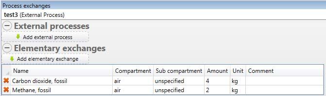
37 2 LCA calculations in all processes: process-specific emissions and external processes Here we explain how the calculations are performed in material processes and external processes, concerning all data specified in the Process exchanges tab. Note that some material processes templates include also emissions happening in the Material transfer tab, these calculations are detailed in Section 3. The steps of characterization, normalization and weighting are always the same, and are thus only explained in Section 2. The example which will be used in Section 2 is presented in Figure S33. Throughout the example we will use an impact category called IPCC 2007, climate change, GWP 100a which has characterisation factors of 1 for carbon dioxide, fossil, air, unspecified and 25 for Methane, fossil, air, unspecified (kg CO 2 -eq/kg). Figure S33: Example used in Section An external process with only process-specific emissions: test3 The external process test3 is presented in Figure S34. It has two process-specific emissions (we call all elementary exchanges in the Process exchanges tab of a process process-specific as they are related to the process being operated): Figure S34: Process exchanges in external process test3 The LCI of an external process such as test3 is presented in Figure S35 and calculated as: SI - 36

38 All elementary exchanges which are directly in the Process exchange tab of test3 are called Process-specific emissions and are simply put directly in the LCI (see the 6 th column below). For each external process used (in test3 none), bring the LCI of the process (explained in Section 2.2 with test2 process). The total column (5 th column) shows simply the sum for all columns for the functional unit for the process. Figure S35: LCI of external process test3 In the characterized impacts, per substance view, the calculation is taking the LCI line by line: for each elementary exchange of the LCI, multiply the total amount by the characterization factor of the impact category. So for test3 characterised impacts are presented in Figure S36 and calculated as: Carbon dioxide: amountofcarbondioxideinlci*characterisationfactorofcarbondioxide = 4*1=4 Methane, fossil: amountofmethaneinlci*characterisationfactorofmethane = 2*25=50 Figure S36: Characterised impacts, per substance, of external process test3 In the characterized impacts, per process view, we take the LCI results column per column: for each subprocess, calculate the total impact as the sum (for all elementary exchanges) of their amount multiplied by the characterization factor. In test3, there is only one sub-process called Process-specific emissions and it is contributing to: amountofcarbondioxideinlci(process specific emissions)*characterisationfactorofcarbondioxide + amountofmethaneinlci(process specific emissions)*characterisationfactorofmethane = 4*1+2*25=54 Results are shown in Figure S37. If test3 was calling another external process, we would do the same calculation for this process (see the example in section 2.2). SI - 37

39 Figure S37: Characterised impacts, per process, of external process test3 2.2 An external process with process-specific emissions and one external process: test2 Figure S38 presents the external process test2. Figure S38: Process exchanges in external process test2 The LCI of test2 has now two subprocesses: Process specific emissions and test3. It is shown in Figure S39 and calculated as: All elementary exchanges which are directly in the Process exchanges tab of test2 are called Process-specific emissions and are simply put directly in the LCI (see the 6 th column below), For each external process used, you have to multiply the LCI of the process by the amount. In our example, test2 uses 2 kg of test3 so in the column test3 we have: o Carbon dioxide: amount(test3usedintest2)* amountofcarbondioxideinlci(test3)=2*4=8. o Methane: amount(test3usedintest2)* amountofmethaneinlci(test3)=2*2=4. Figure S39: LCI of external process test2 In the characterized impacts per substance (Figure S40) the calculation is the following: Carbon dioxide: amountofcarbondioxideinlci*characterisationfactorofcarbondioxide =10*1=10. Methane: amountofmethaneinlci*characterisationfactorofmethane =4*25=100. SI - 38

40 Figure S40: Characterised impacts, per substance, of external process test2 In the characterized impacts per process (Figure S41) the details of each subprocess test3 and processspecific emission are calculated: For the subprocess test3 : amountofcarbondioxideinlciperprocess(test3)*characterisationfactorofcarbondioxide + amountofmethaneinlciperprocess(test3)*characterisationfactorofmethane = 8*1 + 4*25=108 For Process-specific emissions: amountofcarbondioxideinlciperprocess(processspecific)*characterisationfactorofcarbondi oxide + amountofmethaneinlciperprocess(processspecific)*characterisationfactorofmethane = 2*1 + 0*25=2 Figure S41: Characterised impacts, per process, of external process test2 2.3 An external process with process-specific emissions and an external process that uses another external process: test1 Figure S42 presents test1 an external process that uses test2. SI - 39

41 Figure S42: Process exchanges in external process test1 The LCI of test1 is shown in Figure S43(again it has two sub-processes). The calculation is the same as in section 2.2: All elementary exchanges which are directly in the Process exchanges tab of test1 are called Process-specific emissions and are simply put directly in the LCI (see the 6 th column below), For each external process used, you have to multiply the LCI of the process by the amount. In our example, test1 uses 3 kg of test2 so in the column test2 we have: o Carbon dioxide: amount(test2usedintest1)* amountofcarbondioxideinlci(test2)=3*10=30 o Methane: amount(test2usedintest1)* amountofmethaneinlci(test2)=3*4=12 Figure S43: LCI of external process test1 In the characterized impacts per substance (Figure S44) the calculation is: Carbon dioxide: amountofcarbondioxideinlci*characterisationfactorofcarbondioxide =35*1=35 Methane: amountofmethaneinlci*characterisationfactorofmethane =12*25=300 Figure S44: Characterised impacts, per substance, of external process test1 SI - 40

42 In the characterized impacts per process (Figure S45) the details of each subprocess: test2 and processspecific emission are calculated: Test2: amountofcarbondioxideinlciiperprocessoftest2*characterisationfactorofcarbondioxide + amountofmethaneinlciperprocessoftest2*characterisationfactorofmethane = 30*1 + 12*25=330 Process specific emissions: amountofcarbondioxideinlciperprocessofprocessspecific*characterisationfactorofcarbondioxi de + amountofmethaneinlciperprocessofprocessspecific*characterisationfactorofmethane = 5*1 + 0*25=5 Figure S45: Characterised impacts, per process, of external process test1 2.4 A material process uses this external process The scenario presented in Figure S46 has 1000 kg waste (100% vegetable food waste) going to a basic process that uses -3 kg of test1 per MJ energy input and emits 10 kg of carbon dioxide. Figure S46: Process exchanges in basic process The LCI of material processes is similar to the one of external processes (Figure S47): All elementary exchanges which are in the Process exchanges tab of Basic are called Processspecific emissions. Their amount in the LCI is: SI - 41

43 Amount _field * amount_of_the_selected_material_property_in_input_material In our example, we emit 10 kg carbon dioxide per kg total wet weight (here equal to 1000) so we emit: 10*1000=1E4 kg. For each external process used, we get its LCI by: LCI_of_the_external_process * Amount _field *amount_of_the_selected_material_property_in_input_material In our example, we use -3 kg of test1 per MJ of Energy of the input (here equal to 4209 MJ), so we calculate in the 6 th column: o Carbon dioxide: amountofcarbondioxideinlci(test1) *amount(test1usedinbasic) *Energy(input) = 35 *(-3) *4209 = E5 o Methane: amountofmethaneinlci(test1) *amount(test1usedinbasic) * Energy(input) =12 *(-3)*4209 = E5 Figure S47: LCI of basic process In the characterized impacts per substance (Figure S48) the calculation is the following: Carbon dioxide: amountofcarbondioxideinlci *CharacterisationFactorOfCarbonDioxide = E5*1 = E5 Methane: amountofmethaneinlci*characterisationfactorofmethane = E5 *25 = E6 Figure S48: Characterised impacts, per substance, of basic process In the characterized impacts per process (Figure S49) the details of each subprocess: test1 and processspecific emission are calculated: Test1: amountofcarbondioxideinlciperprocess(test1)*characterisationfactorofcarbondioxide + amountofmethaneinlciperprocess(test1)*characterisationfactorofmethane = E5*1 + (-1.515E5)*25 = E6 Process specific emissions: amountofcarbondioxideinlciperprocess(processspecific)*characterisationfactorofcarbondioxid SI - 42

44 e + amountofmethaneinlciperprocess(processspecific)*characterisationfactorofmethane = 9999*1 + 0*25=1E4 Figure S49: Characterised impacts, per process, of basic process 2.5 Normalised and weighted impacts The tabs Norm. imp and Weight. Imp. are very similar to Charact. Imp. with the same per substance and per process views. Figure S50 presents the normalization and weighting factors used. Figure S50: Normalisation and weighting factors used The normalized impacts are obtained by dividing each number in the characterized impacts by the normalization factor of the impact category. In the example of the scenario, we calculate based on characterized impact values (Figure S51): Carbon dioxide: we had -4.32E5 kg so the normalised impact for the category IPCC 2007, climate change, GWP 100 a is: -4.32E5/2 = -2.16E5 PE Methane: we had 3.79E6 kg so normalised impact for the category IPCC 2007, climate change, GWP 100 a is: -3.79E6 /2 = -1.9E6 PE SI - 43

45 Figure S51: Normalised impacts, per substance, of basic process And we also divide the characterised impacts in the per process view (Figure S52). Figure S52: Normalised impacts, per process, of basic process And the weighted impacts are obtained by multiplying each number in the normalised impacts by the weighting factor of the impact category. In the example of the scenario, in the normalised imp. per substance view, we had for: Carbon dioxide: -2.16E5 kg so the weighted impact for the category IPCC 2007, climate change, GWP 100 a is: -2.16E5 *10 = -2.16E6 PE Methane: -1.9E6 kg so normalised impact for the category IPCC 2007, climate change, GWP 100 a is: -1.9E6 *10 = -1.9E7 PE Figure S53 and S54 show the weighted impacts, per substance and per process, respectively. Figure S53: Weighted impacts, per substance, of basic process SI - 44

46 Figure S54: Weighted impacts, per process, of basic process 2.6 Particular case: Material generation In the material generation process, the user can attach the use of an external process to each material fraction by ticking the tick box Include upstream impacts (See Figure S55). Figure S55: Process exchanges in material generation process The LCI calculation is for each external process: LCI = Total_amount *Percentage_field/100 *AmountPerKgFraction *LCI(external_process) In the example, let s calculate for test3: And for test1: Carbon dioxide: 30 *70/100 *2 *4 = 168 kg Methane: 30 *70/100 *2 *2 = 84 kg Carbon dioxide: 30 *30/100 *3 *35 = = 945 kg Methane: 30 *30/100 *3 *12 = 324 kg Figure S56: LCI of material generation process Characterised impact per substance works at process level and at scenario level are calculated as usual by multiplying the total amounts by the characterization factors (Figure S57). SI - 45

47 Figure S57: Characterised impact, per substance, of material generation process Characterised impact per process is calculated by calculating the impact for each external process: sum_for_each_ele_exch [Total_amount *Percentage_field/100 *AmountPerKgFraction *LCI(external_process) *characterization_factor(elem. exch)] In our example, we use an impact category with the characterization factor of 1 for carbon dioxide and 25 for methane, so: o test3: 30 *70/100 *2 *4 * *70/100 *2 *2 *25 = 168*1 + 84*25 =2268 o test1: 30 *30/100 *3 *35 * *30/100 *3 *12 *25 = 945* *25 = 9045 So the characterized impacts are as shown in Figure S58 at process level. Figure S58: Characterised impact, per process, of material generation process 2.7 Particular case: Energy generation This process is similar to material generation process except that we need to back-calculate the Total amount of input. Figure S59: Process exchanges in energy generation process The LCI calculation is for each external process: Total_amount(MJ) *Percentage_field(fraction)/100 /energy%(fraction, MJ/kg) *100/TS%(fraction) *AmountPerKgFraction *LCI(external_process) where energy% and TS% are the properties of the material fraction as found in the library of material fractions. SI - 46

48 For vegetable food waste test3 emits: 30 *70/100 /18.3 *100/23 *2 *[4 kg CO2; 2 kg CH4] = [39.91 kg CO2; kg CH4] Figure S60: LCI of energy generation process The characterised impacts per substance are for CO2: and for CH4: 19.96*25=499. Figure S61: Characterised impact, per substance, of energy generation process Figure S62: Characterised impact, per process, of energy generation process 3 Input-specific emissions in four material processes In this section, we explain how the LCI calculations are performed in the material processes templates that include emissions happening in the Material transfer tab. These emissions are called input-specific. Remember that all processes can have process-specific emissions due to data in the Process exchanges tab (explained in Section I). The 4 processes that can have input-specific emissions are: Substance transfer per fraction. Substance transfer default. Use on land. Emissions to the environment. SI - 47

49 Figure S32 shows the example used where we connect a material generation process each time to a different material process. Figure S63: Scenario used to show the calculations of input-specific emissions This is the composition calculated out of the material generation process. Fraction name Total Wet Weight (kg) TS (kg) Water (kg) VS (kg) Ash (kg) Energy (MJ) C bio (kg) C bio and (kg) C fossil (kg) Ca (kg) Cl (kg) F (kg) Vegetable food waste Office paper Fraction name Vegetable food waste H (kg) K (kg) N (kg) Na (kg) O (kg) P (kg) S (kg) Ag (kg) Al (kg) As (kg) E-06 Office paper E Substance transfer per fraction Figure S64 shows the added emissions to the air unspecified compartment: For Cfossil, 2% goes to the air except for the fraction Vegetable food waste for which it goes at 15%. Al goes at 40% to the air. And we have some process-specific emissions of aluminium and methane, and the use of test3. SI - 48

50 Figure S64: Material transfer for the substance transfer per fraction process Figure S65: Process exchanges for the substance transfer per fraction process Note that we need an interface to explain to EASETECH how Cfossil is emitted: it is emitted as carbon dioxide with a conversion factor of 44/12 (this interface is here by default, just check if you have the right numbers) (see Figure S66). Figure 66: Interface air unspecified SI - 49

51 So the LCI of these Material transfer emissions is calculated for each material property in the dropdown list as: SumForAllFractionsOf[ TransferCoefficientToCompartment(fraction) *AmountProperty(fraction)] * ConversionFactorInInterface So in our example: Carbon dioxide, air, unspecified: [0.15*input.cfossil(vegetablefoodwaste) *input.cfossil(officepaper)] *44/12 = [0.15* * ]*44/12 = kg Aluminium, air, unspecified: [0.4*input.al(vegetablefoodwaste) + 0.4*input.al (officepaper)] *1 = [0.4* * ]*1 = kg And of course the contributions of the Process exchanges tab: Process-specific: o Aluminium, air, unspecified: 0.002*30=0.06 o Methane fossil, air, unspecified: 0.05*30=1.5 Test3: 0.003*30*{2kg CH4; 4 kg CO2} = {0.18 kg CH4; 0.36 kg CO2}. Figure S67: LCI of the substance transfer per fraction process Figure S68: Characterised impacts (subs) of the substance transfer per fraction process SI - 50

52 Figure S69: Characterised impacts (process) of the substance transfer per fraction process 3.2 Substance transfer default We implement the same values as in substance transfer per fraction into a new process based on template substance transfer default. The only difference is that in this process the user cannot specify different transfer coefficients for different material fractions. Figure S70: Material transfer for the substance transfer default process Figure S71: Process exchanges for the substance transfer default process The calculation of characterised impacts also relies on the interfaces. Very similarly to substance transfer per fraction, the LCI of these input-specific emissions is calculated for each material property in the dropdown list as: TransferCoefficientToCompartment * SumForAllFractionsOf (AmountProperty) * ConversionFactorInInterface So in our example: Carbon dioxide, air, unspecified: 0.02*(input.cfossil(vegetablefoodwaste) + input.cfossil(officepaper)] *44/12 = 0.02* ( ]*44/12 = kg SI - 51

53 Aluminium, air, unspecified: 0.4* (input.al(vegetablefoodwaste) + input.al (officepaper)] *1 = 0.4*[ ]*1 = kg And the contributions of the process exchange tab: Process-specific: o Aluminium, air, unspecified: 0.002*30=0.06 o Methane fossil, air, unspecified: 0.05*30=1.5 Test3: 0.003*30*{2kg CH4; 4 kg CO2} = {0.18 kg CH4; 0.36 kg CO2}. Figure S72: LCI of the substance transfer default process Figure S73: Characterised impacts (subs) of the substance transfer default process Figure S74: Characterised impacts (process) of the substance transfer default process SI - 52

54 3.3 Use on land (UOL) The material transfer tab of the UOL process contains all data to calculate the input-specific emissions. Input-specific emissions is the sub-process of all emissions coming from data in the Material transfer tab. As explained in Section I, process-specific emissions are elementary exchanges in the Process exchanges tab and each external process used is a subprocess as well. Figure S75: Material transfer for the UOL process Figure S76: Process exchanges for the UOL process If I call a, b, c, d...n the values input in the 3 tables in the material transfer tab of UOL, the following inputspecific emissions have to be included in the LCI: "Carbon dioxide, non-fossil, air, unspecified": input.cbio * a/100 *(2*M_O+M_C)/M_C "Methane, non-fossil, air, unspecified": input.cbio * b/100 *(4*M_H+M_C)/M_C "Carbon dioxide, fossil, air, unspecified" = input.cbio * c/ 100 *(2*M_O+M_C)/M_C * (-1) "Dinitrogen monoxide, air, unspecified": input.n * e/100 *(2*M_N+M_O)/(2*M_N) "Ammonia, air, unspecified": input.n * f/100 *(3*M_H+M_N)/M_N "Nitrates, water, ground-": input.n * g/100 *(3*M_O+M_N)/M_N "Nitrates, water, surface water": input.n * h/100 *(3*M_O+M_N)/M_N "Phosphate, water, ground-": input.p * l/100 *(3*M_O+M_P)/M_P "Phosphate, water, surface water": input.p * m/100 *(3*M_O+M_P)/M_P SI - 53

55 Note that M_C, M_O, M_P and M_H are constants of the catalogue of constants and they are the molar masses of carbon, oxygen, phosphorous and hydrogen. So the LCI of the subprocess Input-specific is calculated in the example like this: "Carbon dioxide, non-fossil, air, unspecified": ( ) * 80/100 *(2* )/ =15.71 kg "Methane, non-fossil, air, unspecified": ( )* 12/100 *(4* )/ =0.859 kg "Carbon dioxide, fossil, air, unspecified" = ( )* 8/ 100 *(2* )/ * (-1) =-1.57 kg "Dinitrogen monoxide, air, unspecified": ( ) * 2/100 *(2* ) /(2*14.007) = kg "Ammonia, air, unspecified": ( ) * 3/100 *(3* )/ = kg "Nitrates, water, ground-": ( ) * 4/100 *(3* )/ = kg "Nitrates, water, surface water": ( ) * 5/100 *(3* )/ = kg "Phosphate, water, ground-": ( ) * 8/100 *(3* )/ = kg "Phosphate, water, surface water": ( ) * 9/100 *(3* )/ = kg The process test3 has also emissions as explained in part I: 2*30*{4kg CO2; 2kgCH4} ={240 kg CO2; 120 kg CH4}. And in Process-specific emissions, we have one emission of aluminium of 0.8 kg/kg Al = 0.8*( ) = kg. Figure S77: LCI of the UOL process For characterised impacts per substance, let s look only at the impact category Climate change that has characterisation factors for carbon dioxide, fossil, air of 1, for Methane, air of 25, for dinitrogen monoxide of 293: SI - 54

56 Carbon dioxide, fossil: amountofcarbondioxidefossilinlci*characterisationfactorofcarbondioxide =238.4*1 =238.4 Methane, fossil: amountofmethanefossilinlci*characterisationfactorofmethane =120*25=3000 Methane, non-fossil: amountofmethanenonfossilinlci*characterisationfactorofmethane =0.859*25=21.47 kg Dinitrogen monoxide: amountofdinitrogenmonoxideinlci*characterisationfactorofdinitrogenmonoxide = *298= kg Figure S78: Characterised impacts (subs) of the UOL process In the characterized impacts per process the details of each subprocess: test3, process-specific emission are calculated: For the subprocess test3 : amountofcarbondioxideinlciperprocess(test3)*characterisationfactorofcarbondioxide + amountofmethaneinlciperprocess(test3)*characterisationfactorofmethane = 240* *25 =3240 kg For Process-specific emissions: amountofcarbondioxidefossilinlciperprocess(processspecific)*characterisationfactorofcar bondioxide + amountofmethaneinlciperprocess(processspecific)*characterisationfactorofmethane + amountofdinitrogenmonoxideinlciperprocess(processspecific)*characterisationfactorofdini trogenmonoxide = * * *298 =20.84 kg SI - 55

57 Figure S79: Characterised impacts (process) of the UOL process 3.4 Emissions to the environment This process has also a material transfer tab that creates input-specific emissions. In the example following we see that 2 emissions are coming from the Material transfer tab (input-specific emission), while one is coming from the Process exchanges tab (process-specific emission) and we use one external process. So we have 3 sub-processes. Figure S80: Material transfer for the Emissions to the environment process Figure S81: Process exchanges for the Emissions to the environment process The LCI of the emissions happening in the material transfer is calculated for each line as amountofpropertyininput *TransformedAtPercent/100 *ConversionFactor So for our two emissions, it gives: Carbon dioxide, fossil, air, unspecified : input.cbio*80/100*(-44/12) = kg Aluminium, soil, agricultural: input.al*25/100*1= kg SI - 56

58 For the other emissions, it happens as explained in part I: we have an (additional) emission of aluminium of 0.02*30=0.6 kg and emissions from test3 of 2*30*{2kg CH4; 4 kg CO2} = {120 kg CH4; 240 kg CO2}. Figure S82: LCI of the Emissions to the environment process The characterised impact per substance tab shows as usual for each elementary exchange, the total amount multiplied by the characterisation factor. Figure S83: Characterised impacts (subs) of the Emissions to the environment process And the characterised impact per process shows for each subprocess, the sum for all elementary exchanges of amount multiplied by characterisation factor: For the subprocess test3 : amountofcarbondioxideinlciperprocess(test3)*characterisationfactorofcarbondioxide + amountofmethaneinlciperprocess(test3)*characterisationfactorofmethane = 240* *25 =3240 kg For input-specific emissions: amountofcarbondioxidefossilinlciperprocess(processspecific)*characterisationfactorofcar bondioxide = *1 = kg SI - 57

59 Figure S84: Characterised impacts (process) of the Emissions to the environment process SI - 58

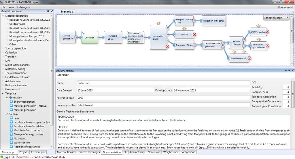
60 PART IV: CASE STUDY In this document are presented screenshots of how the systems were implemented in EASETECH. Please refer to the original paper by Clavreul et al. (2012) for further details. 1 Scenario construction and data input The name of the template used to build each module is provided, as well as screenshots showing the data. Note that parameters were used in some number fields, there value is given in the Section 3 of this Part III. 1.1 Incineration scenario Material generation, based on Material generation template: Collection, based on the Basic process template: Transport, based on the Basic process template: SI - 59

61 Decrease of energy content due to water evaporation, based on the Change of energy content template: Incineration plant, based on the Substance transfer, default template (note that the template Substance transfer, per fraction could have been used instead offering the possibility of giving different values to different material fractions): Transport 500 km (boat), based on the Basic process template: SI - 60

62 Utilisation of fly ashes, based on the Basic process template: Waste water treatment plant, based on the Substance transfer - default template: Transport 50 km, based on the Basic process template: SI - 61

63 Landfill leachate generation, based on the Leachate generation template: Stored ecotoxicity, based on the Substance transfer default template: SI - 62

64 Leachate collection, based on the Mass transfer over years template: Waste water treatment plant, based on the substance transfer default template: SI - 63

65 Emissions to groundwater, based on the substance transfer default template: SI - 64

66 1.2 Anaerobic digestion (AD) scenario Material generation, based on Material generation template: Collection, based on the basic process template: Transport, based on the basic process template: Anaerobic digestion, based on the Anaerobic digestion template: SI - 65

67 CHP gas engine, based on Emissions to the environment template: Addition of water, based on the Water content template: Transport of digestate, based on the Basic process template: SI - 66

68 Use on land, based on the Use on land template: SI - 67

69 2 LCIA methods used Table S2: Environmental impact categories and normalization references of the ILCD recommended methods. References given are first to method, next to normalization references. Impact category Method Unit Climate change Ozone depletion IPCC (Forster et al., 2007) EDIP97 (WMO) (Wenzel et al., 1997) Normalisation factor Year and space of normalisation, reference, remark kg CO 2 -Eq 7730 Laurent et al., 2011a kg CFC-11- Eq 2.05E-2 Laurent et al., 2011a Human toxicity, cancer effects Human toxicity, noncancer effects Particulate matter/ respiratory inorganics Acidification USEtox (Rosenbaum et al., 2008) USEtox (Rosenbaum et al., 2008) Updated from Humbert (2009), from SI of Laurent et al. (2012) ReCiPe (Van Zelm et al., 2008) CTUh 3.25E-5 Laurent et al., 2011b CTUh 8.14E-4 Laurent et al., 2011b kg PM 2.5 -eq 4.71 From SI of Laurent et al. (2012) kg SO 2 -Eq 49.9 Sleeswijk et al., 2008 Eutrophication, terrestrial CML (Guinée et al. 2002) kg NOx-Eq 356 Huijbregts et al, 2003 and CML(2012) 3 Photochemical ozone formation Eutrophication, freshwater Ecotoxicity (freshwater) ReCiPe (Van Zelm et al., 2008) ReCiPe (Van Zelm et al., 2008) USEtox (Rosenbaum et al., 2008) kg NMVOC 52.9 Sleeswijk et al., 2008 kg P-Eq 0.69 Sleeswijk et al., 2008 CTUe 5060 Laurent et al., 2011b Resource depletion, mineral and fossil CML(Guinée et al., 2002) kg antimony- Eq 0.95 Guinée et al., Calculated based on population in EU assumed to: 380 million, and the total value for 1995: 1.4E+11 kg PO43- eq. / yr 3 Uncertainty propagation In this section we present briefly how uncertainty data is input in EASETECH, how systems are parameterized and how results are displayed. 3.1 The table of parameters Parameters are added simply by specifying a name to the parameter, a default value and a list of values to be used when running calculations in sensitivity analysis mode. SI - 68

70 To run the calculations in sensitivity analysis mode, at least one parameter has to be selected and then the user should click on the Run Sensitivity analysis button. SI - 69

71 3.2 Material generation The following figure is a screenshot showing how the waste generation was parameterised using four parameters: the content of plastic in the waste ( plastic ), the water content of the whole waste ( wc ), the lower heating value ( hv ) and the methane potential ( ch4_pot ). It can be observed that to parameterize material generation, we use a different process than the classical one (presented in section Part II, Section 1.3). This process allows free definition of amounts of different properties. The screenshot presents the formulas used for the water content in the 12 material fractions. The pop-up window on the right side shows the table of parameters where all parameters are defined, together with their default value and the list of numbers to be tested. Here each parameter has a list of 1000 values randomly sampled in the distributions defined earlier. This lists of random values were obtained using a small excel macro. 3.3 Material composition calculation The output of this process can be computed and is presented in the next figure. It can be observed that each result field shows the 1000 values obtained as a result of the computation with 1000 values for each parameter. All table results can always be copied and pasted into Excel, which offers simple tools to convert a cell of 1000 values into 1000 cells that can be easily analysed. SI - 70

72 3.4 LCI data in material process In the same way, data of the other processes have been parameterized. Below is presented the example for the CHP gas engine material process. 3.5 Calculation of the characterised impact SI - 71

73 NB: the display of the results will be improved in the future, but it is still possible to make full use of the results by using excel tools. 4 References Clavreul, J., Guyonnet, D., Christensen, T.H., Quantifying uncertainty in LCA-modelling of waste management systems. Waste Management 32, CML (2012). CML-IA Characterisation Factors. Excel spreadsheet [Online] Accessed 31 January 2013 Forster, P., Ramaswamy, V., Artaxo, P., Berntsen, T., Betts, R., Fahey, D.W., Haywood, J., Lean, J., Lowe, D.C., Myhre, G., Nganga, J., Prinn, R., Raga, G., Schulz, M., Van Dorland, R., Changes in atmospheric constituents and in radiative forcing. In: Solomon, S., Qin, D., Manning, M., Chen, Z., Marquis, M., Averyt, K.B., Tignor, M., Miller, H.L. (Eds.), Climate Change 2007: The Physical Science Basis. Contribution of Working Group I to the Fourth Assessment Report of the Intergovernmental Panel on Climate Change. Cambridge University Press, Cambridge, United Kingdom and New York, NY, USA. Guinée, J.B., Gorrée, M., Heijungs, R., Huppes, G., Kleijn, R., Koning, A. de, Oers, L. van, Wegener Sleeswijk, A., Suh, S., Udo de Haes, H.A., Bruijn, H. de, Duin, R. van, Huijbregts, M.A.J., Handbook on life cycle assessment. Operational guide to the ISO standards. I: LCA in perspective. IIa: Guide. IIb: Operational annex. III: Scientific background. Kluwer Academic Publishers, ISBN , Dordrecht, 692 pp. Huijbregts, M.a.J., Breedveld, L., Huppes, G., de Koning, A., van Oers, L., Suh, S. (2003) Normalisation figures for environmental life-cycle assessment. Journal of Cleaner Production 11, Humbert S., Geographically differentiated life-cycle impact assessment of human health. Ph.D. Dissertation, AAT , University of California, CA, USA. Laurent, A., Olsen, S. I., Hauschild, M. Z., 2011a. Normalization in EDIP97 and EDIP2003: updated European inventory for 2004 and guidance towards a consistent use in practice. International Journal of Life Cycle Assessment 16, Laurent, A., Lautier, A., Rosenbaum, R.K., Olsen, S.I., Hauschild, M.Z., 2011b. Normalization references for Europe and North America for application with USEtox characterization factors. International Journal SI - 72