HMLP,MLP and Recurrent Networks for Carbon Monoxide Concentrations Forecasting: A Comparison Studies

Transcription

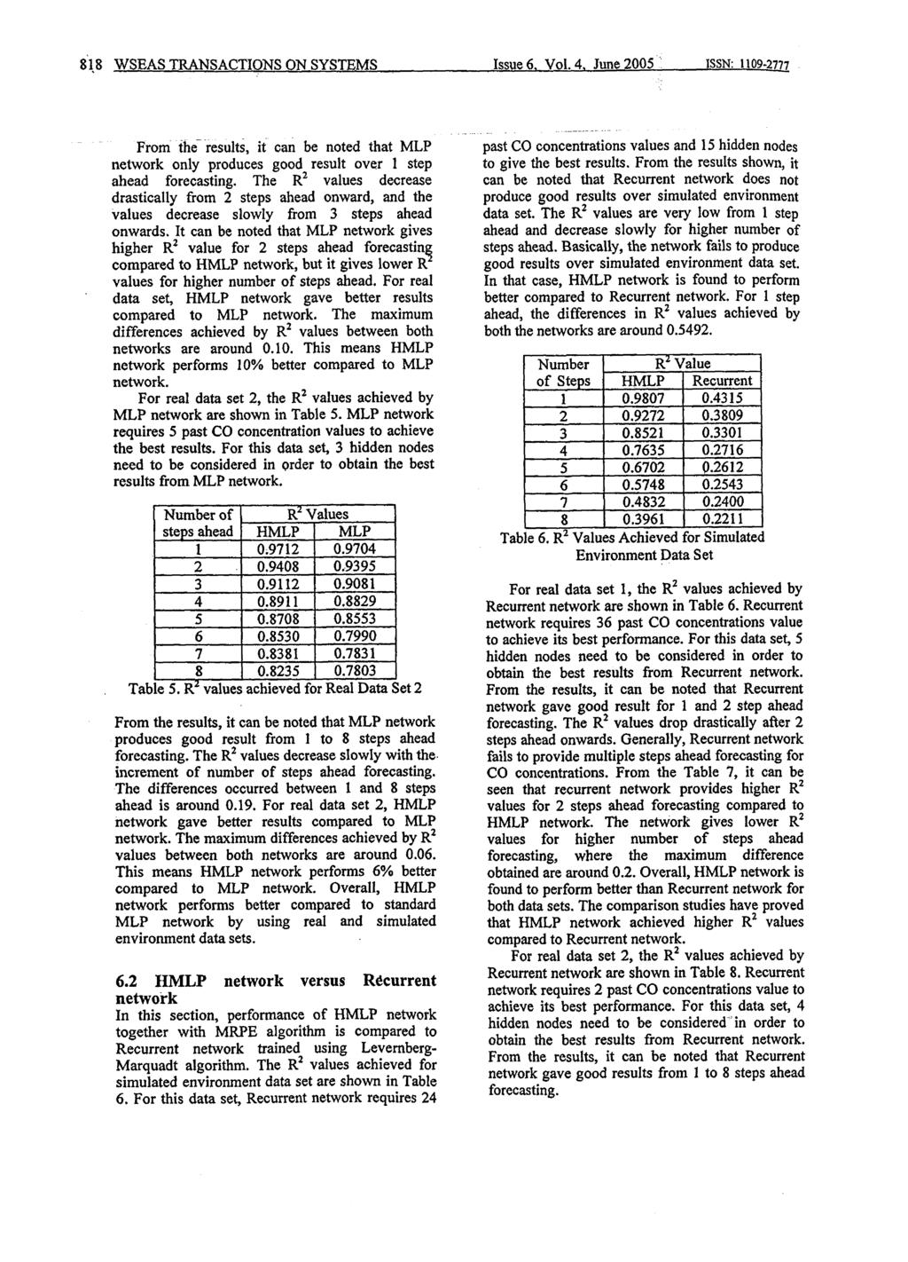
1 812 WSEAS TRANSACTONS ON SYSTEMS ssue 6, Vol. 4. June 2005 SSN: HMLP,MLP and Recurrent Networks for Carbon Monoxide Concentrations Forecasting: A Comparison Studies USHARAN RAJ}, M.Y.MASHOR2, A.N.AL, A.H.ADOM and A.F. SADULLAH Control and ELectronics ntelligent System (CELS) Research Group, School of Electrical & Electronic Engineering, Engineering Campus, University Sains Malaysia, Nibong Tebal, Pulau Pinang, MALAYSA. vsharani@yahoo.com 1.yusof@eng.usm.my2 Abstract: - Carbon Monoxide (CO) is a primary pollutant in urban area, due to the major emission from motor vehicles. Forecasting ofco or other gas pollutants concentration are very important since preventive action can be taken if the forecasted CO level exceeds certain value. Lately, the application of neural networks (NN) becoming very popular for forecasting air pollutants concentration. n order to study this, this paper compares the performance of three model of neural networks, Hybrid Multilayered Perceptron(HMLP) network, Multilayered Perceptron(MLP) network and Recurrent network for CO concentrations forecasting. Two data sets, from simulated based environment and real data obtained from Malaysia Environment Department(ASMA) have been used for modelling and forecasting the CO concentration. For performance comparison, index of coefficient(r2),one step ahead predietion(osa) and multi step ahead prediction(msa) have been used. The study shows ~t HMLP network is the best network for CO forecasting compared to MLP and recurrent networks. Key-Words:- carbon monoxide, forecasting, hybrid multilayered perceptron, multilayered perceptron recurrent network 1 ntrodu'ction The impact of urban air pollution is broad especially towards human beings (WHO, 1987), since it can cause irritation, odour annoyance, acute and long term toxic effects [1]. Carbon Monoxide (CO) is a primary pollutant in urban area, due to the major emission from motor vehicles. CO is produced from incomplete burning of carbon.'contained fuels. According to the Journal of American Medical Association (JAMA), 1500 people die annually due to accidental CO poisoning and people seek medical attention [2]. Forecasting of CO or other gas pollutants concentration are very important since preventive action can be taken if the forecasted CO level exceeds certain value. A lot of researches have been carried out using different methodology on CO concentrations forecasting. One of the methods was by using univariate linear stochastic models based on Box Jenkins modelling technique [3]. This model sufficiently needs long historical data set for model formulation. Another approach was by using BoxJenkins transfer function noise model (TFN) [4]. The forecasting performance was better compared to the first approach presented in [3]. Besides that, Gaussian and regression models were implemented for CO forecasting [5] [6]. n another study, performance comparison between the use of dispersion and stochastic models were carried out. t was reported that stochastic model performed better than dispersion model to predict the hourly mean value of CO concentrations [7]. Lately, the application of neural networks (NN) becoming very popular for forecasting air pollutants concentration. NN have been proved mathematically to be capabje of representing nonlinear systems. A NN known as "Brainmaker" using back propagation algorithm was used to predict CO concentrations with an accuracy of R 2=0.69 [8]. Forecasting on other gases using NN were reviewed since not much of studies have been done specifically on implementation of NN on CO concentrations forecasting. The prediction of hourly time series of NO z was carried out using MLP network, the R 2 obtained was 0.96 [9]. n another study, AR model was used for prediction of N0 2 and NOx concentrations with an accuracy of R 2=O.69 and 0.42, respectively [Ol. The results obtained from [10] were compared with the implementation of MLP network by using the same data set. MLP network was found to perform better

2 WSEAS TRANSACTONS ON SYSTEMS ssue 6. Vol. 4, June2005 SSN: than AR model with an accuracy of R 2 =O.86 and 0.88 [11). n another study, prediction of PM 2.s concentrations was carried out by using multilayer neural network, linear regression and persistence mode~s. The predictions produced by these methods were compared and NN was found to give the best result [12]. n another study, recurrent network with feedback in the hidden layer was used to predict S02 concentration[13]. The network was trained using Levernberg-Marquadt algorithm. The results obtained from recurrent network were compared with those obtained from multivariate regression model. The results indicated that neural network gave better prediction with less residual mean square error than those given by multivariate regression models. n the present study, CO concentrations forecasting performance will be compared between HMLP, MLP and Recurrent networks. The HMLP network is trained using Modified Recursive Prediction Error (MRPE) algorithm. The MLP and Recurrents networks are trained using Levemberg Marquadt algorithm. Their performances are evaluated using R 2 test, OSA and MSA test, respectively. 2 Neural Network Models A hybrid multilayered perceptron with one hidden layer is shown in Figure 1. HMLP. network with one hidden layer can be expressed by the following equation: 1.(1)= t.w~f(tw~v:()+b~)+~w~v:(); -yl fors, k Sa m (1) Yn bias 6 input 't::...,..,!~..~,... ",, \ A multilayered perceptron with one hidden layer can be defined as shown in Equation (2). -.h(t)=t. W~F(t W~V:()+ b}) (2) where w~ x~(") denotes the weights that connect the input and the hidden layers; b} and v: represents the threshold in hidden nodes and input supplied to the network; W;k denotes the weights that connect the hidden and output layer; w~ are the weights connection between input and output layer; niand are the number ofinput nodes and hidden nodes; m represents the number of output nodes while F(.) is an activation function which is normally selected as sigmoidal function. _ - h. h 2 tid bl T e welg ts wi!' wik,wi' an j are unknown, and should be selected carefully in order to achieve minimum prediction error, defined as below: y(k) (3) where YA: (t) and Yk (t) are the actual and predicted output. n this study, recurrent network called as Elman network is applied for the comparison studies. Elman networks are commonly structured as two layer back propagation nenyorks, with the additional feedback connection from the output of hidden layer to its input. The. feedback connection allows the network to ~th recognize and generate time-varying patterns. An Elman network with one hidden layer is shown in Figure 2. \,,,,,,, Fig.2 Elman network u(a: -1) t 1'. l' Standard MLP connection ----» Additional connection Fig.l Hybrid Multilayered Perceptron l" ~, The descriptive equations ofelman network can be written as shown below: XC (k) = x(k -1) xi(k) = j f w:'jxj(k-1) + w:u(k-1)j J lj=l.(4) (5)

3 814 WSEAS TRANSACTONS ON SYSTEMS ssue 6. Vol. 4. June 2005 SSN: N y(k) == L w{xj(k) ;=1 where w:'j is the weight that connects i-th hidden layer neuron and j-th context layer neuron; w; is the weight linking the input neuron u(k -1) and the i-th hidden layer neuron; w{ is the weight that connects output neuron y(k) and the i-th hidden layer neuron; 1(-) represents.activation function in the hidden layer node and N is the number of hidden layer nodes. Usually, sigmoidal activation. function is used for application to modelling nonlinear systems. n the literature, MLP and Recurrent networks were used to perform gasses forecasting. Besides. that, both networks were trained using Levemberg. Marquadt algorithm. That is the main reason both networks were chosen for this comparison studies. 3 Forecasting Performance.n~icator (6) The performance of HMLP, MLP and Recurrent network for CO concentrations.forecasting are evaluated using index ofcoefficient (R 2 ), One Step Ahead Prediction (OSA) and Mean Squared Error (MSE). ndex of coefficient (R2) can be expressed by the following equation: MSE is an iterative method where the model is tested by calculating mean square error after each training step. The MSE at t-th training step is indicated by: EMsE(t,E>(t»=_1 tcy(i)- y(i,8(1»)2 (10) nd ;=1 where EMSE(t,E>(t» and y(i,0(t» are MSE and OSA for a given set of e'stimated parameters 0(t) after t training steps, and n d is the number of data used to calculate MSE. 4 Data Sets The simulated environment data set was collected from a simulated environment in a lab. This setup simulates the conditions ofpartially closed car park or bus station. n this case, cigarettes were used as the CO source for the data c911ection purpose. Figure 3 shows the method used to conduct the CO data collections using cigarette as the source. Three small holes were placed by the side ofthe box, the purpose is to prevent cigarette smoke to be trapped inside the box. The main purpose for the whole setup is to obtain dynatriic CO concentrations measurement For simulated environment data set, 500 data samples were collected with sampling time of 10 seconds. The average, standard deviation and maximum value of CO concentrations measurement for this data set are ppm, ppm and ppm, respectively. R.2 =1- _t_=n.::.,. _ ft, 2:&(t)- y)2 (7) Ventilations where e(t) and yet) are estim:ited error and observed value respectively; y is the average of observed values; n and n t are the first and last.data for testing sample respectively. OSA is a common measure of the predictive accuracy of a model that has been considered by many researchers. OSA can be expressed as below: Yk (t) =f (u(1-1),...u(1 - n ), yet - 1),.... s u y(t - n y ), &(t -1,8),.., &(t - n&,8) and the residual or prediction error is defin~d as: &(t,0) =yet) - yet) where s (.) is a nonlinear function. (8) (9) Cigarette Small holes CO Sensor Fig.3 Data collection from simulated environment The first real data set is referred as industrial data set, which was obtained fro~ Malaysia Environmental Department (ASMA). The data were collected from an industrial area located in Seberang Perai, Penang. These data contains average hourly ofco concentrations measurement,

4 ssue 6, Vol. 4. Ju~e 2005 WSEAS TRANSACTONS ON SYSTEMS GRAPH CO LEVEL VERSUS Nl.JMBER o so SSN: of DATA NUMBliR OF DATA Fig.4 Simulated Environment Data Set which comprises of 1000 data samples. For industrial data set, the average, standard deviation and maximum value of CO concentrations measurement are 7.80 ppm, 3.95 ppm and 27.9 ppm, respectively, The second real data set is obtained from a bus station located in Puduraya, Kuala Lumpur. This data set contains 865 data samples, which were sampled for every 10 seconds. The real data set obtained from Puduraya is shown in Figure 3.7. For this data set, the average, standard deviation and of CO concentrations maximum value measurement are 9.57 ppm, 2.27 ppm and ppm, respectively. 5 CO Concentrations Forecasting using HMLP network n this section, the performance of HMLP network together with MRPE algorithm has been evaluated using one simulated environment data set and two real data sets. n this study, the number of steps ahead to be forecasted has been limited tb eight. Network input series are formed by lagged inputs of CO concentrations level. 5.1 Simulated Environment Data Set in Figure 4. The first 250 data are used to train the network, while the remaining 250 data are used to test the fitted model and to calculate index of coefficient (R2). The network is trained by the following input configuration: gives good results even for higher number of steps ahead forecasting. MSE calculated for the whole data set is shown in Figure 5, which indicates that the network parameters converge rapidly. The MSE converges to an acceptable value after 200 data samples, suggesting that HMLP network only requires about 200 data to be trained properly. Number of R2 Value steps ahead Table 1. R12 Values Acheved for Smulated Environment Data Set S i~ "~-+ ~ i r + ~._~~ ~ ~_.+.~: ~.u~ ~ i ~- f eo... ~.~. -i- ~ } }r... -t... ~... ~_ :,. ; -.~... -t ~ _"} "l"...:..,, t ', 75 t Z.. t.. '& -: t-:-: t r :-~: ~:~! _~:!--~~ _~_ : -:~ t t i: i:: Tr~:rrr:~::rr:rr:::~::f:T:~::r:r: i:so t:~ 1 t}:i::~:+::}::~:::t::~::t::j::~:::}::{::f::(+::..":-.: :"! :....i: :~~ : 'T \ :~ r t- :~~: ':"-! -:H:.~~ ".,j w"w.:ao...,...r. '""'" ~ w_ -..'o.s. Fig.5 MSE for Simulated Environment Data Set 5.2 Real Data Set 1 v(t)=[ yet-) y(t-2) y(t-3) y(t-4) y(t-5)]; For simulated environment data set, HMLP network only requires 5 past CO concentration values to achieve its best results. Number of hidden nodes used are 2, since it gave better results compared to others. The R2 values achieved by HMLP network are shown in Table 1. From the results, it can be seen that HMLP network gives good results over the testing data set. The network The first real data set plot is shown in Figure 6. The first 600 data samples are used to train the HMLP network, while the remaining 400 data are used to test the network. The HMLP network is trained using the following input configuration: v(t)=[ y(t-l) y(t-2) y(t-47) ]; 81

5

6

7

8

9