DYNAMIC THINNING LINES,

Transcription

1 DYNAMIC THINNING LINES, A UNIVERSAL CONCEPT ON PLAICE NURSERY GROUNDS. Nash, R.D.M. 1, Geffen, A.J. 1,2, Witte, J. IJ. 3, and van der Veer, H.W. 3 1 Institute of Marine Research, PO Box 1870 Nordnes, 5817 Bergen, Norway 2 Department of Biology, University of Bergen, PO Box 7800, 5020 Bergen, Norway 3 Royal Netherlands Institute for Sea Research, NIOZ, PO Box 59, 1790 AB Den Burg Texel, The Netherlands

2 1.Nursery ground context 2.What are self-thinning/dynamic thinning and boundary lines 3.The general dynamics of the early life history of plaice 4.Why plaice nurseries are ideal for field studies 5.Examples of self-thinning/dynamic thinning lines in plaice nurseries 6.The relevance of this concept for understanding nursery ground dynamics

3 The dynamics: Numbers of individuals on a nursery ground seasonally increase, individual weights increase, total biomass increases, at some point density begins to fall and then total biomass decreases until the influx of the new year class and the cycle starts again. Numbers Individual weight Total biomass Specifically considering the cases where the population reaches the carrying capacity Time (April to December)

4 From plant ecology: So what is self-thinning? Crowded, even-aged monocultures approach and then track along a line. w = c. d -3/ 2 Where: w = mean weight, d = population density and c = constant Total weight of the population continues to increase as individuals grow, self-thinning occurring until resource limitation or structural or physiological constraints cause a cessation in increase. Total weight then remains constant i.e. carrying capacity is reached and the slope becomes 1 on a log-log plot.

5 In diagrammatic form (plants): Slope = -1 (Constant biomass) Resource limitation, structural or physiological constraint Log mean weight Slope = -3/2 Self-thinning boundary Initial growth Log density

6 The self-thinning rule: as applied to animal populations Expected that a constant biomass/carrying capacity might be applicable i.e. slope = -1. However, relating the slope to metabolic rates i.e. raised to 0.75 or a slope of 1.33 is probably more applicable for mobile animals. This gives: logw = c - 4/3logd Proviso: Assumes that the food/resource (F) input to the population remains constant throughout the growth of the cohort. However, the possibility that F remains constant for animal populations is much less likely.

7 Self-thinning in animal populations: Theoretical considerations Amount of food increases with time. Log Mean weight df +ve dt Steepens the s-t line (<-4/3 e.g. 3/2, -2 etc) Log density Adapted from Begon et al. 1986

8 Self-thinning in animal populations:theoretical considerations Consumption outstrips food growth df ve dt Less steep (>-4/3 e.g. 1) Log Mean weight Log density Also: df/dt can change due to the behaviour of the population e.g. territoriality or migration Adapted from Begon et al. 1986

9 Boundary lines Species boundary lines: a line beyond which combinations of density and mean weight are not possible (see Weller 1990, Begon et al. 2006) Essentially the carrying capacity of the environment. Food-limited cohorts The carrying capacity is determined by the balance between growth and mortality

10 Self-thinning in food-regulated populations [energetic equivalence theory] Carrying capacity is where βg=m (intercept). Growth (g) Mortality (m) Log (N) m βg F Lower food production affects either βg or m. Equilibrium energy flow (F) is lower in habitats with lower food production. If food production keeps changing then the slope will change. In seasonal environments the slope is not constant Log (w) Progress along the thinning lines are equal. Bohlin et al. 1994

11 The case of energy flow (F) varying with body size Log (F/k) Log (N) Curvilinear thinning lines Diet changing with body size Food for intermediate body sizes having a higher rate of production Log (w) Bohlin et al. 1994

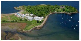
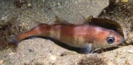
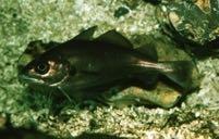
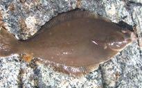
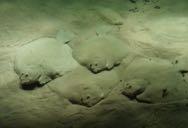
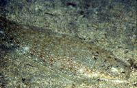
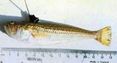
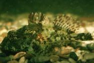
12 Why choose juvenile flatfish and plaice in particular? Kristineberg Marine Research Station Port Erin Marine Laboratory Dunstaffnage Marine Laboratory NIOZ

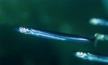
13 Early life history trajectory for North Sea plaice (Pleuronectes platessa) 28 Potential Egg Production Irish Sea North Sea SSB Hatch 24 Log e Abundance 20 Eggs Larvae Metamorphosis Begining July Start Age 1 From : Beverton & Iles (1992) Beverton (1995) 16 Settlement period Nursery ground Over-wintering PELAGIC DEMERSAL Jan 25-Feb 25- Mar 22- Apr 20-May 17-Jun 15-Jul 12- Aug 9-Sep 7-Oct 4-Nov 2-Dec 30-Dec Day of year Nash & Geffen (20??)

14 Dynamics of a nursery ground Supply of larvae/juveniles Increasing size of individuals Decrease in abundance due to mortality Decrease in abundance due to emigration Phases (idealised): Time

15 Expected trajectory of log mean weight and log population density Log mean weight Emigration Food limitation? Self-thinning Log density Growth Settlement Inter-annual variations on nursery grounds Differences between nursery grounds Log mean weight High production year Log mean weight High carrying capacity Log density Low production year Log density Low carrying capacity

16 Plaice nursery grounds with time series of abundance and mean weights

17 Juvenile plaice: Density versus mean weight Mean weight (g) Expected slope = Tralee (open) PE Bay (closed) PE 1995 PE 1996 PE 1997 PE 1998 PE 1999 Mean weight (g) Port Erin Bay Slope = Mean weight (g) Tralee Bay (Scotland) Slope = Density (m -2 ) Density (m -2 ) Density (m -2 ) Nash et al MEPS 344

18 Other plaice nursery grounds 1000 Average weight (AFDW) per plaice (g) Slope = Slope = Swedish Bays Self-thinning 1991 Self-thinning Density (per sq m) Filey Bay density varies x30 Firemore Bay density varies x6

19 Drop trap Swedish Beaches (1978, 79, 91, 92) 2 1,5 1 0,5 0-1,5-1 -0,5 0 0,5 1 1,5 Data Thinning Constant biomass Linear (Data) -0,5 y = -0,778x - 0,3228 R² = 0, ,5

20 Dutch Wadden Sea ( , 1991, , 2007, 2009, 2014) Mean weight (g) 1 0,1 0,01 0,0001 0,0010 0,0100 0,1000 1, ,0000 Density (m-2)

21 Varying boundary lines? 1970s 1990s 2 2 All data 2 1,5 1 y = -1,5681x - 1,4881 R² = 0,4154 1,5 1 y = -1,3426x - 1,8036 R² = 0,7464-0,5-1 -1,5-2 y = -1,371x - 1,6416 R² = 0, ,5-1 -0,5 0 0,5 1 At a given density there was a reduction in mean weight of: 55% between 1970s and 1980s 68% between 1980s and 1990s But an increase 26% - between 1990s and 2000s Overall a reduction of: 80% - between 1970s and 2000s 1,5 1 0, ,5-1 -0,5 0 0, s 0,5-0,5-1 -1,5-2 -0,5-1 -1,5-2 y = -1,7151x - 1,9001 R² = 0, ,5-1 -0,5 0 0, ,5 1 0, ,5-1 -0,5 0 0, s -0,5-1 -1,5-2 -2,5 0,5-0,5-1 -1,5-2 y = -1,1195x - 1,565 R² = 0, ,5-1 -0,5 0 0,5 1 1,5 1,5 1 0,5

22 Comparisons between nurseries a question of productivity/differing carrying capacities? Maximum densities observed on the nursery grounds 4,0 3,0 2,0 Log Mean weight (g) 1,0 0,0-1,0-2,0-3,0-2,0-1,5-1,0-0,5 0,0 0,5 1,0 1,5 Log Density (m-2) Tralee Swedish DT 1970s PEB 1980s 2000s 1990s Max Location Thinning intercept density (m -2 ) Tralee 1,02 14,4 Swedish 0,25 10 PEBay -0,23 3 Filey Bay 1,2 Firemore Bay 1,2 WS2000s -0,15 0,8 WS1990s -0,5 0,8 WS 1970s -0,9 1 WS 1980s -1 0,4

23 Self-thinning (a single species consideration) A cohort over time, ages and the individuals grow. The resource requirements i.e. space and food increase and thus competition will also increase. The risk of dying increases. If individuals die, density decreases, competition decreases which affects growth this in turn affects competition and thus growth and so the cycle continues. In animal populations the rules seen in plant populations may be more questionable due to: Variable resource supply Possible other factors e.g. territoriality etc rather and only the food supply Begon et al However, they provide a framework for modelling density, with a growth (and thus mortality rates) on nursery grounds, through the summer and autumn months.

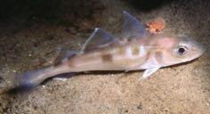
24 The dynamics of nursery grounds can be very complex with numerous inter-specific interactions occurring Predatory crustaceans Predatory gadoids Competitors Residents

25 In summary: 1. Inter-annual variability in supply of juveniles to nurseries considerable variability in density 2. Dynamic thinning occurring after settlement ceases 3.Variable slopes for dynamic thinning often 4/3 4. Mechanism uncertain 5. The influence of emigration on the reduction in density uncertain 6. Upper boundary lines vary between nurseries 7. Upper boundary lines vary over time

26