CENTRE FOR APPLIED MACROECONOMIC ANALYSIS

Transcription

1 CENTRE FOR APPLIED MACROECONOMIC ANALYSIS The Australian National University CAMA Working Paper Series January, 2011 THE ROLE OF ENERGY IN THE INDUSTRIAL REVOLUTION AND MODERN ECONOMIC GROWTH David I. Stern Arndt-Corden Department of Economics, Crawford School of Economics and Government, ANU and CAMA Astrid Kander CIRCLE and Department of Economic History, Lund University CAMA Working Paper 1/2011

2 1 The Role of Energy in the Industrial Revolution and Modern Economic Growth David I. Stern Arndt-Corden Department of Economics, Crawford School of Economics and Government and Centre for Applied Macro-Economic Analysis, Australian National University, Canberra, ACT 0200, AUSTRALIA Astrid Kander CIRCLE and Department of Economic History, Lund University, Lund, SWEDEN November 2010 Abstract The expansion in the supply of energy services over the last couple of centuries has reduced the apparent importance of energy in economic growth despite energy being an essential production input. We demonstrate this by developing a simple extension of the Solow growth model, which we use to investigate 200 years of Swedish data. We find that the elasticity of substitution between a capital-labor aggregate and energy is less than unity, which implies that when energy services are scarce they strongly constrain output growth resulting in a Malthusian steady-state. When energy services are abundant the economy exhibits the behavior of the modern growth regime with the Solow model as a limiting case. The expansion of energy services is found to be a major factor in explaining the industrial revolution and economic growth in Sweden, especially before the second half of the 20th century. In the latter period, labor-augmenting technological change becomes the dominant factor driving growth. JEL Codes: O13, O41, Q43, Q56 Key Words: Unified growth theory, energy, Industrial Revolution, economic growth Acknowledgements: We thank Stephan Bruns, Paul Burke, Creina Day, Helena Johansson, Jack Pezzey, Peter Warr, and Fredrik Wilhelmsson for providing useful comments, and Lennart Schön for providing unpublished data.

3 2 Introduction In this paper, we seek to explain how energy could play a major role in the long-run growth of the economy and be crucial in explaining the Industrial Revolution yet occupy a small share of the costs of production in today s advanced economies. We develop a simple model that extends Solow s (1956) neoclassical growth model to include energy and estimate its parameters using data from the past two centuries in Sweden. The model shows that the expansion of energy services was the most important factor explaining growth until the second half of the 20 th century when labor-augmenting technical change becomes paramount. Additionally, the model can explain the historical decline in the energy cost share seen in the Swedish data (Figure 1), which appears to be a typical feature of economic development (Kander et al., forthcoming). We emphasize that our model is far from a complete theory of growth but we believe that this model will help explain how energy is very important for growth but that models of modern economic growth can yield good results while essentially ignoring it. Many energy and ecological economists (e.g. Cleveland et al., 1984; Ayres and Warr, 2005, 2009, Hall et al., 2003), economic historians (e.g. Wilkinson, 1973; Wrigley, 1988; Allen, 2009), and geographers (e.g. Smil, 1994) believe that energy related innovations and the growth in the supply and quality of energy play a crucial role in economic growth, as well as being an important component in explaining the Industrial Revolution. Time-series analysis (Stern, 1993, 2000) shows that energy is needed in addition to capital and labor to explain the growth of GDP. But mainstream economics research has tended to downplay the importance of energy in economic growth. The principal models used to explain the growth process (e.g. Aghion and Howitt, 2009) do not include energy as a factor of production. As our model will show, this omission is probably because energy has been very abundant in recent decades in developed economies and its cost share low, so that the constraints imposed by energy availability on economic growth are weaker than they were in the past and it can implicitly be assumed that energy supply increases in the long-run as needed. On the other hand, there is a large literature examining whether non-declining per capita consumption or utility is feasible (i.e. whether the economy is sustainable) in the face of the non-renewable nature of some resources starting with Solow (1974), Dasgupta and Heal (1979), and Stiglitz (1974), through Aghion and Howitt (1998), to recent contributions such as Di Maria and Valente (2008) among others. There is also a literature on the environmental impact of growth with

4 3 important contributions by Aghion and Howitt (1998), Jones and Manuelli (2001), and Brock and Taylor (2005) among many others. These models do not, however, usually specify whether the resources in question are energy or non-energy resources. An exception is Tahvonen and Salo (2001), who model past and possibly future energy transitions between renewable and non-renewable energy explicitly. In their model, the dominant energy vector switches from renewable to non-renewable energy and back again over the course of economic development. The drivers of these shifts are the different price paths of the two sources of energy over the course of economic development. Though this latter paper is much more historically realistic than most work in resource economics, it does not directly address the importance (or not) of energy in economic growth and its role in the Industrial Revolution. There are currently two principal mainstream economic models of the transition from the preindustrial economy to the modern growth regime. The endogenous technical change approach represented by Galor and Weil (2000) and Lucas (2002) emphasizes the role of human capital and fertility decisions in the transition. The rate of technological change in Galor and Weil s model is a function of the size of the population and the level of education. Initially, there is a steady-state equilibrium that has a low rate of technological change and a low level of education. As population grows, a second fast technological change and high education equilibrium emerges, which eventually is the only equilibrium (Galor, 2005). Energy and resources play no explicit role in this approach. The underlying assumption is that energy was never a significant limiting factor, but was always relatively abundant, as it is today. The second approach, represented by Hansen and Prescott (2002), assumes that two technologies are available the Malthus technology, which depends on a land input and has decreasing returns to combined labor and capital and the modern Solow technology that has constant returns to capital and labor combined, and does not face any natural resource constraints. Initially, the use of the Solow technology is unprofitable and the economy experiences pre-industrial stagnation. The transition to the modern growth regime starts when technological change first makes the operation of the modern technology profitable. The economy is initially a dual economy with modern and traditional sectors. Over time, the modern sector grows and the traditional sector declines as capital flows from the traditional

5 4 to modern sector. Hansen and Prescott (2002) note that the Solow technology probably uses fossil fuels in place of land, but they do not model energy explicitly. Economic history provides qualitative models of the Industrial Revolution, where the breaking of the constraints of the organic economy plays a fundamental role. Wrigley (1988, 2010) stresses that the shift from an economy that relied on land resources to one based on fossil fuels is essential to the Industrial Revolution and could explain the differential development of the Dutch and British economies. Both countries had the necessary institutions for the Industrial Revolution to occur but capital accumulation in the Netherlands faced a renewable energy resource constraint, while in Britain domestic coalmines in combination with steam engines, at first to pump water out of the mines and later for many other uses, provided a way out from the constraint. Early in the Industrial Revolution, the transport of coal had to be carried out using traditional energy carriers, for instance by horse carriages, and was very costly, but the adoption of coal-using steam engines for transport, reduced the costs of trade and the Industrial Revolution spread to other regions and countries. This explanation emphasizes the low substitutability between the essential inputs of capital and energy, with newly available punctiform energy sources (coal) relaxing the constraint on capital accumulation. With restricted energy supplies, based on areal-bound resources, capital accumulation faced rapidly diminishing returns. Pomeranz (2001) makes a similar argument, but addresses the issue of the large historical divergence in economic growth rates between England and the Western World on the one hand and China and the rest of Asia on the other. He suggests that shallow coal-mines, close to urban centers together with the exploitation of land resources overseas were very important in the rise of England. Ghost land, used for the production of cotton for the British textile industry provided England with natural resources, and eased the constraints of the fixed supply of land. In this way, England could break the constraints of the organic economy (based on land production) and enter into modern economic growth. Allen (2009) places energy innovation centre-stage in his explanation of why the industrial revolution occurred in Britain. Like Wrigley and Pomeranz, he compares Britain to other advanced European economies of the time (the Netherlands and Belgium) and the advanced economy in the East: China. England stands out as an exception in two ways: coal was

6 5 relatively cheap there and labor costs were higher than elsewhere. Therefore, it was profitable to substitute coal-fuelled machines for labor in Britain, even when these machines were inefficient and consumed large amounts of coal. In no other place on Earth did this make sense. Many technological innovations were required in order to use coal effectively in new applications ranging from domestic heating and cooking to iron smelting. These induced innovations sparked the Industrial Revolution. Continued innovation that improved energy efficiency and reductions in the cost of transporting coal eventually made coal-using technologies profitable in other countries too. On the other hand, Madsen et al. (in press) find that, controlling for a number of innovation related variables, changes in coal production did not have a significant effect on labor productivity growth in Britain between 1700 and But as innovation was required to expand the use of coal this result could make sense even if the expansion of coal was essential for growth to proceed. 1 Our aim is to examine a simple model of the breaking of the constraints imposed by dependence on the organic economy and the shift towards the modern growth regime. For the sake of simplicity we base our model on Solow s (1956) neoclassical growth model. We add an energy input that has an elasticity of substitution of less than unity with capital and labor, while we set the elasticity of substitution between capital and labor at unity. Additionally, we allow for biased technical change, so rather than treating technology as a single index of total factor productivity there are two indices one augments labor and the other augments energy. 2 Energy-augmenting technical change represents all methods of obtaining more economic output from a given energy input without substituting capital and labor for energy or augmenting the other inputs through technological change. This includes both greater energy efficiency in producing existing products and the development of new products such as steam engines and computers that use energy in new, more productive ways. 3 The 1 Additionally, as Madsen et al. s (in press) regression is in first differences, they can only measure the direct short-run impact effect of changes in energy use. Also there could be problems with endogeneity. We address both issues by using a cointegrating regression in levels. 2 A similar approach is taken in a number of recent resource economics papers such as Di Maria and Valente (2008) and Fröling (in press). 3 In the empirical work we account for the effect of shifts in the mix of energy carriers on energy quality by employing a Divisia index of energy use rather than the simple sum of heat units. Though such indexation methods account of the shift from lower quality (less productive) to higher quality (more productive) fuels they do not take account of the increased productivity of individual fuels (Stern, 2010a),

7 6 Industrial Revolution involved both innovations that effectively augmented the supply of energy, for instance the smelting of iron ore with coke instead of charcoal, increases in the energy supply (coal from deep mines), and improvements in the quality of the energy sources used. We can think of effective energy services as the product of the level of the energy supply, the quality of that energy, and the level of energy-augmenting technology. In common with Brock and Taylor (2010), we assume that technological change is exogenous, not because that is a realistic assumption but because that is the simplest model of economic growth on which we add new complications. It is also more reasonable for modeling the development of a follower country such as Sweden than it would be for modeling the development of the British economy, which took the lead in the Industrial Revolution. Why do we use a general CES production function rather than the more commonly used Cobb-Douglas function? After all, if the elasticity of substitution is between energy and capital-labor is unity and the energy supply is constant then energy will act as a constraint on growth in the same way that a fixed land supply constrains growth in Hansen and Prescott s (2002) model. The main reasons why we allow that for the elasticity of substitution to differ from unity are as follows. First, it enables a simple model with only one sector rather than the two sectors in Hansen and Prescott, while allowing a change in the degree to which energy constrains growth within that sector over time. Second, thermodynamic considerations suggest that production of a given level of output has minimum energy requirements (Stern, 1997). When the elasticity of substitution is less than unity there is a finite minimum energy requirement for any level of output irrespective of the level of capital employed. Third, empirical evidence points in this direction. Koetse et al. (2008) carry out a meta-analysis that finds that the mean elasticity of substitution is less than one in the empirical studies that they analyzed. Fourth, the cost share of energy in Sweden, a country for which we have data from 1800 till the present, fell over time (Figure 1). This is not possible for a single sector economy with an elasticity of substitution of unity (Cobb-Douglas technology), which implies that cost shares are constant. The extent of the fall from an energy cost ratio of 90% of GDP or more in 1800 to close to 10% of GDP today, does not support a unit elasticity. Fifth, we cannot distinguish between labor-augmenting innovations 4 and energy-augmenting innovations in a Cobb-Douglas technology. In the constant elasticity of substitution (CES) 4 As we assume that capital and labor combine in a Cobb-Douglas function, laboraugmenting innovations are also of course capital-augmenting innovations.

8 7 technology labor-augmenting technical change does not augment the energy supply. Thus we can examine the role of energy-augmenting technical change in the Industrial Revolution and long-run growth. An alternative approach, often used in resource economics, is to think of energy services as being produced by capital and energy, which then combine with labor to produce final output. We do not adopt that set-up because it assumes that the elasticities of substitution between energy and labor and between capital and labor are equal. In a preindustrial society a major use of energy was as food for workers such that there may also be limited substitutability between labor and energy. Furthermore, our model nests the Solow (1956) growth model as a special case, which is useful for expository purposes, while the alternative model does not. Fröling (in press) develops a unified growth model that incorporates an energy input. Her model is an example of the Galor and Weil (2000) approach as population growth drives the rate of endogenous technical change and there is no real energy constraint on production. In her model, energy services are a (high) CES aggregate of coal and biomass, which are each produced using labor alone. So the size of the labor force also drives energy availability. Innovative activity, which also only uses labor, leads to the accumulation of two stocks of knowledge one of which enhances TFP in the production of final output while the other enhances the productivity of coal in producing energy services. Biomass is only distinguished from coal in that knowledge cannot enhance its productivity. Thus the shares of biomass and coal change over time. Labor is used in five separate activities and research expenditures in each sector are assumed to be a constant share of final output much as saving is a constant share of output in the Solow model. Population evolves according to Jones (2001) demographic model. As final output is produced by a Cobb-Douglas function of labor, aggregate energy services, and a fixed quantity of land, the model cannot reproduce the decline in the energy cost share, which we see in our data, whereas our model can. Additionally, there is no capital stock in Fröling s model while our model can exploit the available capital data. The next section of the paper outlines our model and its properties. This is followed by the discussion of the Swedish data we use to estimate parameters and the econometric methods

9 8 and results. We use the estimated parameters in a historical simulation, which provides a kind of growth accounting of the importance of the various factors on economic growth in Sweden. The paper concludes with a discussion section. Theoretical Model Our model aims at explaining a major shift in economic history. This can be thought of as a shift in the economy s steady-state from one with low output to one with high output due to an increase in the availability of effective energy services. Similarly, continued expansion of effective energy services allowed a higher rate of economic growth then in the pre-industrial period because expanding energy services continually moved the steady-state to higher levels of output. This section of the paper examines the properties of this model. What are the properties of the steady-state and what are the effects of the various variables on the level of output and growth in the steady-state? What are the implications for the evolution of marginal products, income shares, energy intensity, and productivity growth? The Model Omitting time indices for simplicity, the model consists of two equations: Y = ( γ 1/σ V (A β L L β K 1 β ) φ + γ 1/σ E (A E E) φ ) 1 φ (1) ΔK = sy δk (2) Equation (1) is a nested CES production function that embeds a Cobb-Douglas function of capital (K) and labor (L) in a CES function of the capital-labor aggregate and energy (E) that determines gross output Y. 5 φ = σ 1, where σ is the elasticity of substitution between energy σ and the capital-labor aggregate. The share parameters γ Ε and γ V sum to unity. 6 A L and A E are the augmentation indices of labor and energy. Here we ignore changes in the quality of the inputs, which will be addressed in the empirical section of the paper. The levels of labor and energy are assumed to be exogenous. Equation (2) is the equation of motion for capital that assumes, like Solow (1956), that the proportion of gross output that is saved is fixed at s and 5 The Cobb-Douglas function is a CES function with an elasticity of substitution of unity. 6 The fact that these parameters are fixed does not mean that the cost share of energy is fixed. As shown in equation (24), the cost share is also a function of other variables and parameters. This parameterization ensures that for γ V A L β L β K 1 β = γ E A E E the level of output is invariant to the elasticity of substitution. γ V and γ Ε are only identifiable econometrically if a restriction is placed on the augmentation indices.

10 9 that capital depreciates at a constant rate δ. 7 These assumptions can be relaxed in a more complete model of growth. Equation (1) explicitly ignores land and materials. In the pre-industrial economy energy was mostly produced by the agricultural and forestry sectors that used land as an input. The model represents that land input by the energy input, which later also includes fossil fuels. This is a tremendous simplification but allows us to show the effect of a minimal modification of the Solow growth model. By ignoring materials we assume that they can be aggregated together with energy in the energy input. We choose to assume that labor and capital combine in a Cobb-Douglas function so that as σ -> 1 and γ Ε -> 0 the model asymptotically tends towards the original Solow model, which appears to be a reasonable model of the modern economic growth regime. In this case, K and Y will grow in the steady-state at the rate of laboraugmentation. Additionally, the shares of capital and labor in GDP will be constant, in accord with one of Kaldor s (1957) stylized facts despite their non-constant shares of gross output. Also if σ < 1 and γ Ε > 0, as A E E the term γ 1/σ E (A E E) φ 0, so that the model tends towards the Solow model but with a higher capital stock and output due to the coefficient γ 1/σ V, as discussed below. The production function (1) has two limits to substitution (Stern, 1997). First, energy is essential to production and if σ < 1 a minimum quantity of energy is required to produce any given level of output. This is a static limit to substitution. Second, energy is required to produce capital and as long as δ > 0, maintenance of the capital stock requires an ongoing energy input. Therefore, there is an additional limit to the degree to which capital can be substituted for energy. This can be thought of as a dynamic limit to substitution. Steady-State and Comparative Statics All the following results assume that 1 > σ > 0. We can find the steady-state of the system by substituting (1) into (2) and setting ΔK = 0, which gives the following equation in the steady-state capital stock, K : ( δ /s) φ K φ + γ 1/σ V ( A L L) βφ K φ( 1 β ) + γ 1/σ E (A E E) φ = 0 (3) 7 It makes more sense to think of saving as a fixed share of GDP as we do in the empirical exercise in the paper, but it complicates the theoretical part of the paper, and does not change anything qualitatively.

11 10 There is no general analytical solution to (3), so apart from special cases such as β = 2/3, 0.5, 1/3 etc. we must use numerical methods to find the steady-state solution. For β = 0.5, there are two roots to the equation: az 2 + bz + c = 0 (4) where z = K 0.5φ. The solutions for the steady-state capital stock are: 1 K = 2 δ /s γ ( ) φ V ( ) 0.5φ 2 ± γ /σ V ( A L L) φ 1/σ + 4γ E 1/σ A L L (( δ /s)a E E) φ 2 φ (5) As 4γ E (( δ /s)a E E) φ > 0, there is only one positive solution for K. As A E E increases, equation (5) converges to: lim A E E K = sγ V δ 1/σφ 1 β AL L (6) 1/ ( βσφ which is equal to the steady-state capital stock in the Solow model multiplied by γ ) V > 1. Therefore, the steady-state capital stock is higher than in the Solow model. As σ 1 and γ V 0, (6) converges to the Solow steady-state capital stock. However, when energy is scarce and substitutability is low the steady-state capital stock defined by (5) or (3) can be less than the Solow steady-state capital stock. Is the negative root of (5) relevant? In other words, can the system collapse to zero output or have more than one steady-state in the general case? The marginal product of capital is: Y K = 1 β ( )γ V 1/σ A L L /K ( ) βφ Y /K ( ) 1 φ (7) In the Cobb-Douglas case φ = 0 and as K approaches 0 the derivative approaches infinity, guaranteeing that: s Y K > δ (8) in the neighborhood of the origin and that, therefore, there is a single stable equilibrium. However, in general, CES functions other than the Cobb-Douglas function do not satisfy the Inada conditions (Barelli and de Abreu Pessoa, 2003). It is possible for extreme parameter values low savings rate, high depreciation rates, high levels of β and low levels of σ - that

12 11 (8) is not met neither near the origin nor for any positive value of K so that there is no positive equilibrium level of capital. 8 The derivative of (7) with respect to K is: 2 Y K = ( 1 β)γ 1/σ 2 V A L L ( ) βφ Y φ K φ βφ 1 ( 1 φ) Y ( ) Y K + φ βφ 1 K (9) As shown in Appendix A, this second derivative is negative, so that if there is a positive steady-state equilibrium it is unique and stable. Though there is no general solution for the steady-state capital stock, we can apply the implicit function theorem to (3) to determine how each factor affects the steady-state capital stock. As at the steady-state equilibrium δ > s Y / K, the term δ s Y / K is positive and the derivatives and their signs are as follows: K s = Y δ s Y / K > 0 (10) K γ E = sy 1 φ K φ = sy φ δ s Y / K ( ( )) φ ( A E E /γ E ) φ A β L L β K 1 β / 1 γ E σφ(δ s Y / K ) ( ) (11) γ V (A β L L β K 1 β /γ V ) φ ln(a β L L β K 1 β /γ V ) + γ E (A E E /γ E ) φ ln(a E E /γ E ) lny Y φ (12) K β = sy1 φ (A L L β K 1 β ) φ γ 1/σ V (lnl lnk ) δ s Y / K (13) K δ = K δ s Y / K < 0 (14) K E = sy1 φ γ 1/σ E A φ E E φ 1 > 0 (15) δ s Y / K K L = sy1 φ βγ 1/σ V A βφ L L βφ 1 (1 β )φ K > 0 (16) δ s Y / K K = sy A L 1 φ βγ 1/σ V A βφ 1 L ( L β K (1 β ) ) φ δ s Y / K > 0 (17) K = sy1 φ γ 1/σ E A φ 1 E E φ > 0 (18) A E δ s Y / K The results show that a higher savings rate always increases the size of the steady-state capital stock while higher depreciation rates result in smaller equilibrium stocks of capital. 8 See Klump and Preissler (2000) for a similar result for the capital-labor low constant elasticity of substitution production function.

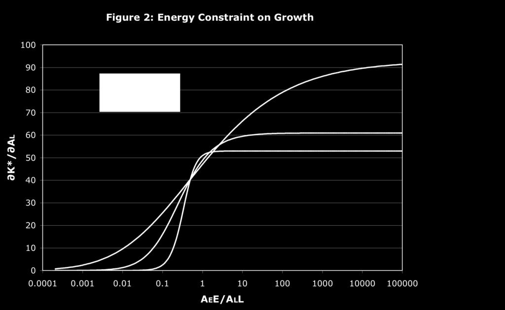
13 12 Equation (11) shows that the sign of the energy share parameter depends on the relative abundance of energy etc. When energy is abundant putting more weight on energy increases the steady-state capital stock. But when energy is scarce the reverse is true. This is not dependent on whether the elasticity of substitution is greater or smaller than unity. Klump and Preissler (2000) demonstrate that for β = 0 (12) is positive. Simulations find that this is true in general. Equation (13) shows that the effect of the labor share of income depends on the capital/labor ratio. When labor is abundant relative to capital, increasing its share increases the optimal capital stock and vice versa. The effects of the two non-capital inputs labor and energy and their augmentation indices on the steady-state capital stock are always positive as one might expect. Steady-State Growth In the Solow model, steady-state growth in output per capita is possible as long as labor can be augmented by technological change. In the current model, as in the Solow model, as there are constant returns to scale, increasing the labor force by the same amount as the other inputs has no effect on output per capita. However, also because of constant returns to scale, increasing the population without increasing the energy supply reduces output per capita as in the conventional Malthusian-Ricardian model. In the standard Solow model with a Cobb- Douglas production function, labor-augmenting technical change cannot be distinguished from factor neutral technical change. However, in the case of the CES function, (1), technical change that augments labor does not augment energy and vice versa. To explore this result we can plot the derivative of the steady-state capital stock with respect to the augmentation index of labor (17) against the augmentation index of energy. We set β = 0.5, γ = 0.1, s = 0.1, δ = 0.05, L = 1, E = 1, A L = 1, determine K according to (5) and allow the elasticity of substitution and A E to vary. Figure 2 shows the results. For low elasticities of substitution and low levels of the energy augmentation index (or equivalently energy supply), laboraugmenting technical change has little effect on the optimal capital stock. For high levels of the energy augmentation index (or equivalently energy supply) labor-augmenting technical change has a positive effect of constant magnitude. Allowing for more substitutability results in more of an effect of labor augmentation at low levels of energy, as we would expect. For a Cobb-Douglas function without energy K / A L is a constant with a value of 40 in this case. So the addition of the energy input reduces the effect of labor augmentation on growth at low levels of energy and increases it at high levels of effective energy.

14 13 Equation (5) is homogenous of degree one in the augmentation indices. Therefore, if both rates of technological change are equal, the capital stock will grow at the same rate in the long-run and due to constant returns to scale, so will gross output. Appendix A proves that this is true more generally too. The response curves in Figure 2 are, therefore, a function of A E E / A L L. If the energy supply is fixed and there is no energy augmentation the economy eventually converges on a steady-state where K and Y are constant despite ongoing augmentation of labor. 9 The only way out of this constraint is for there to either be an increase in the energy supply, for there to be energy -augmenting technical progress, or for a switch to higher quality fuels to occur. The Industrial Revolution involved all of these. Input Prices, Income Shares, and Energy Intensity The marginal products of the three inputs are given by equation (7) and: Y L = βγ 1/σ V ( A β L K (1 β ) ) φ ( Y /L β ) 1 φ (19) Y E = γ 1/σ E A φ E ( Y / E) 1 φ (20) The output elasticities of the three inputs are, therefore, given by: lny lnk = ( 1 β 1/σ )γ V lny lnl = βγ 1/σ V (( A L L) β K (1 β ) /Y) φ (21) (( A L L) β K (1 β ) /Y) φ (22) lny ln E = γ 1/σ E ( A E E /Y) φ (23) and GDP is given by: G = Y lny lnl + lny lnk = γ 1/σ V Y 1 φ A L L (( ) β K ) (1 β ) φ (24) As explained above, if effective energy A E E is growing as fast as the rate of labor - augmenting technical progress in the steady-state output will too and the energy output elasticity (24) will be constant over time. In order to find a declining energy cost share as seen in Sweden from 1800 to the late 20 th century (Kander, 2002), the rate of expansion of effective energy (rate of energy -augmenting technical change plus the rate of increase in 9 Even if there was no depreciation of capital, so that the capital stock kept growing, the low elasticity of substitution production function requires a minimum input of effective energy for any given output level and so growth would eventually halt anyway.

15 14 energy quality (Cleveland et al., 2000) plus the rate of increase in the energy supply has to have been greater than the rate of labor -augmenting technical progress (and increase in labor quality), assuming competitive markets. This would result in output growing slower than effective energy supply. Equations (21), (22), and (24) show that, despite potential change in the share of energy in gross output over time, the shares of capital and labor in GDP remain constant at 1- β and β. Finally, energy intensity is given by: E G = e = γ V 1/σ Y 1 φ E (( A L L) β K ) (25) (1 β ) φ To understand the factors that affect the time path of energy intensity we take derivatives: e = E(φ 1)Y φ 2 Y / A E A 1/σ E γ V A L L (( ) β K ) (26) (1 β ) φ As φ < 0, energy augmentation has a negative effect on energy intensity much as we would expect. Labor augmentation has an apparently ambivalent effect as both terms inside the brackets in (27) are negative but the second is subtracted from the first: e A L = ( ) E (φ 1)Y φ 2 A βφ L Y / A L φβy φ 1 βφ 1 A L (27) γ 1/σ V L βφ K (1 β )φ Simulations suggest that the derivative really may be positive or negative, depending on the degree of substitutability and other factors. This is unexpected, as it is often argued that general TFP growth lowers energy intensity (e.g. Stern, 2002). In the current model, however, labor-augmenting technical change could, in theory, lower GDP while raising gross output. Finally, increased energy supply can have positive or negative effects: e E 1+ E(φ 1) Y / E = Y 1 φ A L L (( ) β K ) (28) (1 β ) φ When energy is scarce and the marginal product of energy is very high it is likely to be negative and vice versa. Productivity Growth Some ecological economists (e.g. Ayres and Warr, 2005, 2009; Cleveland et al., 1984; Hall et al., 2003) have argued that either energy, properly measured, accounts for most apparent productivity growth, or that technological change is real but innovations increase productivity

16 15 by allowing the use of more energy. So what is the role of energy in productivity growth in our model? If the gross output elasticities remain constant over time, GDP will grow as fast as gross output and energy makes no contribution to growth beyond its share of gross output. But if the output elasticity of energy falls over time GDP will grow faster than gross output and it will largely be energy -augmenting technical change and increased energy supply that would be responsible for this phenomenon. It is easier to explore the implications for labor productivity rather than total factor productivity: G L = l = Y1 φ A βφ L L βφ 1 K (1 β )φ (29) For the Cobb-Douglas case this collapses to Y/L and only labor, capital, and labor-- augmenting technical progress contribute to the growth in labor productivity. To examine the general case we take the time derivative of (29). Using the standard notation convention for time derivatives: l Y = (1 φ)a βφ L L βφ 1 K (1 β )φ Y φ A E A E + Y E E + l A L A L + l L L + l K K (30) The first term on the right hand side indicates the contribution of changes in effective energy to labor productivity, which is positive as φ <1. A study that ignored the first term in (30) would over-estimate the contribution of labor augmentation to labor productivity growth. On the other hand, labor augmentation and capital deepening still play a role in increasing labor productivity in our model. Data We use data for primary energy input. For all the modern energy carriers, such as coal, oil, and electricity, there are reliable historical statistical sources, such as import and production data. For traditional fuels such as fuelwood, food, and fodder this is not the case, so estimates must be made. We use the estimates developed by Kander (2002) who also tabulates the quantity and price series for the modern energy carriers. Firewood prices are sensitive to assumptions of how much energy a particular amount of wood contained, and this varies. We use the lower of the two firewood prices in Kander (2002). The GDP data comes from the national historical accounts for Sweden (Krantz and Schön, 2007). To obtain gross output, we followed Berndt et al. (1993), adding the value of energy to the value of GDP.

17 16 The labor series is from the same Historical National Accounts (number of employees). The capital stock data has not yet been published, but was kindly provided to us by Lennart Schön. It is based on the investment series that are part of the Historical National Accounts. The method for turning this into a capital stock is the usual perpetual inventory method using straight-line depreciation of buildings over 50 years and of machinery over 25 years. In other words a building investment loses 2% of its original value every year, while machinery investment loses 4%. This means that even though investment data is available already from 1800 the stock of capital is only available from Therefore, although there are energy series and GDP series available from 1800 on we can only estimate the full model from 1850 onwards. From 1800 to 2000, GDP per capita rose 17-fold. Population increased from about 2.3 million in 1800 to around 9 million in The ratio of energy value to GDP fell from around 90% in 1800 to just above 10% in These are very dramatic changes that the model needs to explain. We aggregated the various energy inputs using both simple addition of heat units and using Divisia indexation 10, which accounts for the effect of shifts in the mix of fuels used on the effective energy services provided. Energy carriers vary in quality, which is reflected in their productivity and, therefore, their prices and so higher quality carriers such as electricity represent a much larger share of energy costs than of heat content. In order to avoid infinite percentage changes, we ignore the change in the quantity of oil, natural gas, and primary electricity in the first year each energy carrier was introduced. We also assumed that the prices of oil and gas before prices are first available were equal to the price in their first year of availability deflated by the GDP deflator, which is quite a rough assumption. Still, this method only affects a few years in our series, and the cost shares of these energy carriers were very small in the first few years after their introduction. The ratio of this index of energy volume to the sum of heat units is a measure of energy quality. By this measure, energy quality increases two and a half-fold over the two centuries. Most of the increase is focused in the 20 th century where the higher quality modern energy carriers become increasingly significant. 10 Annually chained Paasche-indexation produced similar results to Divisia aggregation.

18 17 Econometric Model and Results Where possible, we estimated the parameters used in the simulation model in the next section. Because technological change affects the share of energy in gross output we must estimate simultaneously the rate of technological change together with the elasticity of substitution or fix the value of one of the parameters, a priori. Because there are two technology trends we need at least two equations to identify the trends (Harvey and Marshall, 1991). Equations that are potentially useful include the production function (1) and energy output elasticity (23) replacing the elasticity on the left-hand side of (23) with the share of energy in gross output. Following Kim (1992) we use the log of the ratio of the cost share of energy to the cost share of capital-labor as we expect this variable to be more normally distributed. We also take logarithms of (1) due to the high level of heteroskedasticity in the untransformed gross output series. To account for measurement units a different parameterization of the scale constants in the production function is used. The model is given by: ln S Et = lnγ E + σ 1 1 S Et σ ln A β ln A Et Lt + ln Q t E t [ ( ) β ln L t ( 1 β)lnk t ] + ε Et (31) lny t = lnγ 0 + σ σ 1 ln σ 1 (A β L β t K 1 β σ t ) + γ Lt E (A Et Q t E t ) σ 1 σ + ε Yt (32) where Q is the quality index of energy, and ε Et and ε Yt are random error terms. Edvinsson (2005) provides gross profit ratio data for Multiplying this rate by the capital stock series and dividing by GDP shows that the capital share has fluctuated around a mean of 23% of GDP. Data for the Swedish manufacturing sector supplied by Lennart Schön show an average wage share of 72% from 1875 and Both of these are fairly low values for the income share of capital. Most estimated values for other countries are in the range of 0.3 to 0.5 (Mankiw et al., 1992). Still, there is no reason not to use the data we have, so we, therefore, treat β as a known parameter with a value of The states of technology in (32) and (33) are unobserved and likely to be correlated with the explanatory variables (Stern, 2010b). If this is the case, parameter estimates will be biased. Instrumental variables using lagged values of the explanatory variables is unlikely to be an effective method as the lags will also be correlated with the state of technology. As well as estimating static models we use the approach of adding leads and lags of the first differences

19 18 of the explanatory variables (Stock and Watson, 1993; Choi and Saikkonen, 2010). Two leads and lags of the first differences are used as well as the contemporaneous first difference of the logs of energy volume and the capital-labor aggregate. We use the Newey and West (1987) approach to computing the covariance matrix of the coefficients for all models using two correlated lags. We estimate models with constant rates of energy and labor augmentation as well as models with rates that are different in each half century. Assuming a constant rate of augmentation,ln A it = τ i1 t 1850 where t 1850 is a time trend equal to zero in 1850 and i refers to either labor or energy. For variable rates of augmentation we use the following formula: ln A it = τ i1 t τ i2 t τ i3 t 1950 where t 1900 is a time trend equal to zero for years up till and including 1900 and t 1950 is equal to zero up to and including 1950 and increasing by one per year from 1951 on. Table 1 presents the results. All regressions use annual data from 1853 to 1998 because of the leads and lags required by the DNLLS estimator. Estimates of the coefficients of the lags and leads variables are omitted. It is safe to assume that all the key time-series in the model have stochastic trends and so we do not engage in formal testing of this hypothesis. We apply three cointegration tests to the residuals. Choi and Saikkonen (2010) provide the first cointegration tests for the general non-linear model. The null hypothesis of their test is cointegration in which case the residuals of the equations are stationary. The test uses the same basic test statistic as the KPSS test (Kwiatkowski et al., 1992) but applies a Bonferroni procedure to subsamples of the residuals. Critical values are provided by Hong and Wagner (2008). Full details are given in Appendix B. We also use the Phillips and Ouliaris (1990) test of the null hypothesis of non-cointegration. Though, these tests do not formally apply to the non-linear case, equation (31) is linear in the variables. The estimated parameters are fairly consistent across the various specifications. Adding the leads and lags of first differences of the explanatory variables does not make much difference to the results. Models with variable rates of technological change have, however, slightly lower elasticities of substitution and the dynamic estimates slightly higher. The Phillips and Ouliaris cointegration tests fail to reject the null of non-cointegration for either equation for both specifications of the constant rate of technical change model. The null of noncointegration can be rejected for both equations and both specifications for the variable rate of technological change model. Only one of the Choi and Saikkonen test statistics is

20 19 significant at the 10% level rejecting the null of cointegration for the cost share ratio equation in the constant rate of technological change model. However, it is clearly apparent that the all the test statistics are much larger for the constant rate of technological change model, indicating that the variable rate model fits the data better. The rate of energy augmentation is significantly slower after 1900 than before but does not change significantly after 1950 (model 3S) or increases slightly (3D). Labor augmentation is negative before 1900, is significantly positive after 1900 and is found to accelerate further after A negative augmentation for labor seems to not make any sense, unless working hours reduced in the 19 th century, which they did not. However, we cannot distinguish between labor- and capital-augmenting technical change and Holmqvist (2003) and Schön (2004) found that TFP growth was negative in Swedish industry and manufacturing during this period of capital deepening in the late 19 th century. Another possible explanation is that the elasticity of substitution between capital and labor is actually less than unity, which recent research suggests (Chirinko, 2008). However, we lack good data on the cost shares of capital and labor and so have not pursued that direction. We found, however, that imposing a lower elasticity of substitution between capital-labor and energy resulted in non-negative labor augmentation is each period. This suggests that our estimates of the elasticity of substitution, which range from 0.64 to 0.69 might be somewhat conservatively high. Simulation of a Model Economy To give more insight into how the model behaves and understand the historical role of energy in growth, in this section we simulate the behavior of a model economy that fits the available data for Sweden over the 19 th and 20 th centuries. The simulation solves for the capital stock and GDP endogenously given exogenous labor, energy supply, and energy quality. We used the parameter values from model 3D in Table 1. In order to get the simulation to approximate the actual data reasonably well, we need to allow the savings rate to change over time. Since the capital series were constructed by assuming a straight-line depreciation of structures over 50 years and of machines over 25

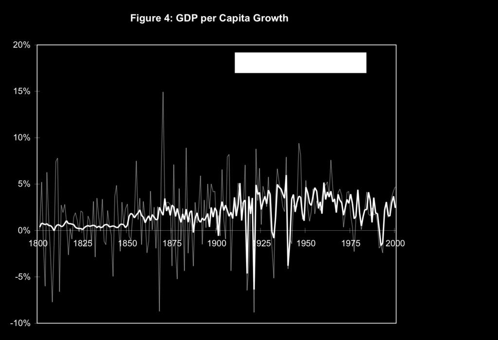
21 20 years, we assume a constant rate of depreciation of 6%. 11 Then we can calculate the savings rate from the following equation: s t = ΔK t + δk t 1 G t (33) The estimated savings rate rose from 6% in 1850 to around 22% in For the period , we do not have capital stock or labor data, so the simulation is more speculative than in subsequent years. We need to calibrate the initial capital stock, and the rates of labor and energy augmentation and saving, and the size of the labor force between 1800 and We assume that prior to 1850 the labor force was the same 38.6% of the population that it was in We interpolated the 1800 population from Maddison s data. Population grew by 0.6% p.a. between 1700 and We estimate the population in 1800 as 2.3 million and, therefore, the labor force was 885,000. We assumed a zero rate of labor -augmenting technical change prior to A negative rate would have given a better fit to the data, however. We assumed that the initial capital stock was in steady-state equilibrium as given by (2) but with GDP in place of gross output and then calibrated the savings rate so that the projected capital stock in 1850 was at the observed level. This gave a savings rate of 5.6% for the first half of the 19 th century and a capital stock of SEK 336 million in prices in We then set the rate of energy augmentation over so that GDP equaled its observed value in The estimated rate is 1.03%. The estimated cost share of energy in gross output in 1800 is then 0.41 against the observed value of A negative rate of labor augmentation (of around 1% per annum) together with a higher rate of energy augmentation would raise the cost share of energy closer to the observed value while predicting GDP in 1800 correctly. Alternatively, a lower elasticity of substitution could be imposed. Figure 3 shows simulated GDP per capita (black line) and observed GDP (colored line). Simulated GDP per capita rises from SEK( ) 157 in 1800 to 5,230 in The fit is fairly good despite technical change being constant for 50 years at a time. However, observed GDP is much more volatile (Figure 4). There are two sources of volatility in our model labor and energy supply. The volatility of the labor series is extremely variable. For 11 Depreciation of the remaining value will be 4% per annum for 25 year-old structures and 8% for 25 year-old machines. Simplifying by assuming that the capital stock is constant and composed of 50% machines and 50% structures results in a depreciation rate of 6%.

22 21 long periods the series grows at a constant rate and at other times grows very erratically. The energy series has low volatility before about 1875, as a result of the way in which it was constructed. In that period, traditional fuels still played a major role in the Swedish economy, and their use was estimated based on data on population, the number of cattle, and trends in the use of fuelwood, food, and fodder, without any attempt to produce annual fluctuations in response to climate or other short-run variations. The series match each other quite well from around As we go further back in time the simulated series is less and less volatile, but the volatility of observed GDP increases. GDP per capita grows at 0.7% p.a. before 1850 and at up to 2.5% per annum after 1900 (Table 2). The step up in the growth rate around 1850 is quite noticeable in Figure 4. Energy supply grew very slowly up till 1850 and at an increasing rate after that. Energy quality only grew at a rapid rate after 1900, when electricity, coal, and oil increased their shares. Energy augmentation peaked during but was already at 1.3% per annum in This makes historical sense as the energy efficiency of stoves, steam engines, and iron smelting all improved rapidly in the 19 th Century (Kander, 2002). The total effective energy supply grew at 1.9% before 1850 and from 3.3% to 4.2% per annum after Most importantly, though labor augmentation was non-positive before 1900, the economy was growing due to the increase in effective energy supply. Throughout the two hundred year period both the growth rate of effective energy supply and GDP per capita exceeded the rate of labor augmentation. Figure 5 displays all three input prices over time. The rate of return on capital rises from 24% in 1800 to a peak of 34% and then falls to 9% over time. 12 Wage rates rise continuously. Energy prices (per heat unit) are flat till the late 19 th century before falling somewhat. Energy prices per effective unit of energy fall throughout the period. The price of an effective unit of labor has increased continuously over time but at a slowing rate. 12 The high marginal product of capital in the 19 th century seems paradoxical at first glance. In what sense was limited energy a barrier to growth if additional capital accumulation could seemingly have increased output so much? First, the share of capital in gross output in 1800 was only half what it is today. Despite the higher marginal product, the output elasticity was lower. Second, capital demand was rather inelastic. The marginal product of capital fell rapidly as the capital stock was increased resulting in a small gain in capital income for increasing the capital stock. Holding energy supply constant, the marginal product of energy rose strongly as the capital stock increased. As a result the increase in GDP was much less less than 5% of the increase in capital - than the increase in gross output.

23 22 Next, we simulate the economy under some counterfactual scenarios to further understand the effects of changes in the quantity and quality of the inputs and technological change on output. These are not realistic scenarios as the variables we treat as exogenous here include savings rates, population growth rates, and rates of technological change that would in reality react to the changed scenario. Table 3 presents results for the scenarios. Holding energy use constant at 1800 levels results in the economy growing by 0.5% less per annum over the two centuries. GDP per capita would not have been much lower in 1850 but by 2000 it would have only been 42% of its actual level. Energy quality has less effect. Because energy quality only improved in the 20 th century, GDP per capita is the same in 1900 under this scenario as under the base case. By 2000, GDP per capita would have been 21% lower. Under the no energy augmentation scenario, GDP per capita would have been a lot lower in the late 19 th century as well as the 20 th century, ending at just 24% of actual levels in Energy innovation was, therefore, more important in the 19 th century than increasing energy supply or quality, while the latter became more important in the 20 th century though energy innovation was still important. When we hold all three of these factors constant so that the effective energy supply remains at the 1800 level, the economy collapses, with income per capita declining by 0.5% per annum and GDP per capita at 1/3 of its 1800 level by GDP itself is lower too. We also test the effects of savings and labor augmentation on growth. If there had been no labor augmentation, the growth rate of the economy would have been 0.6% lower than in actuality. GDP per capita would, though, have been higher through 1900 due to the negative rate of labor augmentation that we estimated in the late 19 th century. Labor augmentation becomes important in the late 20 th century so that GDP per capita would have been only 28% of its 2000 level under this scenario. Most of the empirical growth literature uses data from this latter period and, therefore, mainstream growth theory emphasizes labor-augmenting technical change. Holding the savings rate constant at 5.6% per annum, has no effect on GDP per capita in 1850 as this was the estimated constant savings rate for the first half of the 19 th century. It has similar effects to constant energy quality after that. In summary, each of the three components of effective energy supply had a major impact on economic growth in Sweden over the last couple of centuries. Without an increase in

24 23 effective energy supply it is hard to imagine any economic growth could have occurred at all. On the other hand, labor augmentation had important effects in the second half of the 20 th century as the economy became more freed from energy constraints and increased savings also had important effects. Energy related innovations are necessary and crucial, but the other factors also play a role. Discussion The model presented in this paper should not be seen as a complete model of economic growth but rather as an exploration of a mechanism whereby energy can constrain or enable growth depending on its relative abundance. The simulation showed how innovations in the energy field were both a trigger of modern economic growth in Sweden and have been important in enabling growth ever since. The model we have presented is capable of incorporating a time-varying energy cost share, by allowing a low elasticity of substitution between energy and the other factors of production (labor and capital). Of course, alternative explanations of the data need to be considered. One possibility is change in the structure of production. Looking at the sectors included in GDP we see that no sector of the economy today has as high an energy cost share as the economy as a whole did in In 1800 Agriculture was the largest sector at 40% of GDP followed by services and manufacturing industry (Krantz and Schön, 2007). This mix changed little over most of the rest of the 19 th Century. However, in the 19 th Century a large part of the economy consisted of subsistence activities such as growing crops for on-farm consumption and collecting firewood, not all of which are included in GDP. Since many tasks in the economy were carried out in the household and since workers needed to be kept alive, all this energy should be included in a full account of energy and economic growth, and it is incorporated in our estimates of energy use and our measure of gross output. This sector of the economy was very energy-intensive. The share of the household sector in total energy use declined in the 19 th Century though it was fairly constant in the 20 th Century (Kander, 2002). Furthermore, the share of economic activity that occurred within the home vs. in formal markets has also increased. So this structural change may explain part of the reduction in the cost share of energy. However, the share of consumer expenditure represented by energy has also declined considerably so that the shift of economic activity from households to the market cannot explain the entire decline in the energy cost share.

25 24 Another hypothesis is that the economy consists of two sectors with Cobb-Douglas technologies a traditional sector with a very high energy cost share and a modern sector with a low energy cost share, along the lines of Hansen and Prescott (2002). This idea is harder to refute. Relevant evidence in favor of the low elasticity of substitution hypothesis is that the elasticity is clearly less than unity in the short-run as witnessed in the oil price shocks of the 1970s. Additionally the energy cost share does seem to have declined further after animal power use effectively ended. The latter could be seen as an indicator of the traditional organic economy. As mentioned in the introduction, energy could have acted as a constraint on growth before the Industrial Revolution even if the elasticity of substitution between energy and the other inputs is unity. However, in the face of labor-augmenting technical change, energy would only constrain growth in such a model if population grew in response to higher income in Malthusian fashion. The model in this paper will be stuck in stagnation even if population does not respond to rising income, as is the case in the modern world, unless effective energy services can be increased. What would change if we added a Malthusian population mechanism to our model? In the Malthus sector of the Hansen and Prescott model a technological improvement initially increases the potential steady-state income. The population response to that increased income results in diminishing returns because there are decreasing returns to capital and labor combined and, therefore, income per capita returns to the previous level. In practice it depends on how rapid technological change is and how quickly population responds to higher income per capita. In the Solow sector there are constant returns to labor and capital and hence the Malthusian effect does not occur. In the model is this paper, if population responds to higher income, the Malthusian effect should occur in response to factor neutral technical change to the same extent as in the Malthus sector of the Hansen and Prescott model as long as the energy supply does not increase alongside the increase in population. This is because there are decreasing to returns to capital and labor combined in our model. The implications of our model for the future are very different to those of the Hansen- Prescott model. In their model, society has freed itself from the constraints of resource limitations. In our model, the economy is still latently constrained by resources. Future

26 25 growth depends on either maintaining increases in energy supply or augmenting energy through technological change. Despite its simplicity, the model in this paper may already explain quite a lot about the history of energy and the economy. Appendix A Uniqueness and Stability of Steady State The second derivative of the production with respect to capital is: 2 Y K = ( 1 β)γ 1/σ 2 V A L L ( ) βφ Y φ K φ βφ 1 ( 1 φ) Y ( ) Y K + φ βφ 1 K For σ > 1 this is obviously negative. For σ < 1, the first term in the brackets is positive and the second negative and so it is not clear that the derivative is always negative. From (7) and (1) the expression in the brackets is: ( 1 φ) Y + φ βφ 1 K ( ) Y K ( ) φ ( = 1 φ) ( 1 β)γ 1/σ V ( A L L) β K 1 β γ 1/σ V (A β L L β K 1 β ) φ + γ 1/σ E (A E E) φ ( 1 φ) ( 1 β) β Multiplying the term in the brackets on the RHS here by γ V 1/σ (A L β L β K 1 β ) φ + γ E 1/σ (A E E) φ gives: βγ 1/σ V (A β L L β K 1 β ) φ (( 1 φ) ( 1 β) + β)γ 1/σ E (A E E) φ < 0 Therefore, the second derivative of Y is negative too and if a steady state exists it is unique and stable. Y K Steady State Growth Assuming that L and E are held constant for simplicity, the percentage rate of change in the steady-state capital stock is given by: K ˆ = lnk ln A L A ˆ L + lnk ln A E ˆ A E where hats indicate percentage or proportional rates of change. If the two rates of technological change are equal then substituting in the expressions for the two elasticities based on (19) and (20) and the formula for the marginal product of capital (8), gives: sy 1 φ βγ 1/σ K ˆ V A β L L β K (1 β ) = δk s( 1 β)γ 1/σ V A β L L β K (1 β ) ( ) φ + γ E 1/σ A E φ E φ ( ) φ Y 1 φ A ˆ noting that at the steady-state equilibrium δk = sy we have:

27 26 Y 1 φ βγ 1/σ K ˆ V A β L L β K (1 β ) = Y ( 1 β)γ 1/σ V A β L L β K (1 β ) ( ) φ + γ E 1/σ A E φ E φ ( ) φ Y 1 φ A ˆ Substituting in the expressions in equations (22) to (24) and simplifying yields: K ˆ lny / lnl + lny / ln E = A ˆ 1 lny / lnk which due to constant returns to scale is equal to the rate of technological change. Also due to constant returns to scale of the production function (1), gross output also increases at the same rate. Appendix B The form of the KPSS cointegration test statistic in the linear case is (Shin, 1994): κ = T 2 s 2 T t=1 t j=1 e j 2 where T is the time-series sample size, s 2 is a consistent estimator of the long-run variance of the residuals from the long-run relationship and the estimated residuals of the long-run relations are denoted e. In the nonlinear case, the distribution of this statistic depends on unknown parameters. Choi and Saikkonen (2010) show that if instead the statistic is based on sub-segments of the residual series of a length that meet certain conditions then a limiting distribution function can be derived and tabulated. For a subsegment of length b starting with observation i, we have: κ i,b = b 2 2 s i,b i+b 1 t= i t j= i e j 2 To improve the power of this test statistic, Choi and Saikkonen propose a Bonferroni procedure. M test statistics are computed for segments starting i 1 to i M and the statistic with the maximum value is selected and used as the test statistic: κ max i,b = max( κ,...,κ i1,b i M,b) The appropriate critical values for the 5% and 10% levels are tabulated by Hong and Wagner (2008) for values of M from 2 to 40. The segment length b is chosen as follows: 1. A range of possible segment lengths b k from [T 0.7 ] to [T 0.9 ] is chosen where [x] denoted the integer part of x.

28 27 2. For each of these possible values of b compute the 5 test statistics κ max i,bk 2,...,κ max i,bk Compute the standard deviation c k of these statistics. 4. Choose the block size that minimizes c k. Given b: 1. M = [ T /b] +1 if T/b is not an integer and M = [ T /b]otherwise. 2. Then i 1 = 1, i 2 = T -b+1, i 3 = b+1, i 4 = T -2b+1 etc. 2 To estimate the long-run variance s i,b we follow Hong and Wagner (2008) using the Newey- West spectral window and a lag length of [ 4( b /100) 0.25 ]. This lag length gave much better results in the Monte Carlo study of Choi and Saikkonen (2010) than an alternative longer laglength that they also tested. References Aghion, P. and P. Howitt (1998), Endogenous Growth Theory, MIT Press, Cambridge, MA. Aghion, P. and P. Howitt (2009), The Economics of Growth, MIT Press, Cambridge MA. Allen, R. C. (2009), The British Industrial Revolution in Global Perspective, Cambridge University Press. Ayres, R. U. and B. Warr (2005), Accounting for growth: the role of physical work, Structural Change and Economic Dynamics 16, Ayres, R. U. and B. Warr (2009), The Economic Growth Engine: How Energy and Work Drive Material Prosperity, Edward Elgar, Cheltenham. Barelli P. and S de Abreu Pessoa (2003), Inada conditions imply that the production function must be asymptotically Cobb-Douglas, Economics Letters 81, Berndt, E. R., C. Kolstad, and J-K. Lee (1993), Measuring the energy efficiency and productivity impacts of embodied technical change, Energy Journal 14, Brock W. A. and M. S. Taylor (2005), Economic growth and the environment: A review of theory and empirics, in P. Aghion and S. N. Durlauf (eds.) Handbook of Economic Growth, North Holland, Volume 1B, Brock W. A. and M. S. Taylor (2010), The green Solow model, Journal of Economic Growth 15,

29 28 Chirinko, R. S. (2008), σ: The long and short of it, Journal of Macroeconomics 30, Choi, I. and P. Saikkonen (2010), Tests for nonlinear cointegration, Econometric Theory 26, 2010, Cleveland C. J., R. Costanza, C. A. S. Hall and R. K. Kaufmann (1984), Energy and the U.S. economy: A biophysical perspective, Science 225, Cleveland C. J., R. K. Kaufmann, and D. I. Stern (2000), Aggregation and the role of energy in the economy, Ecological Economics 32, Dasgupta, P. and G. Heal (1974), The optimal depletion of exhaustible resources, The Review of Economic Studies, Vol. 41, Symposium on the Economics of Exhaustible Resources (1974), pp Di Maria, C. and S. Valente (2008), Hicks meets Hotelling: the direction of technical change in capital resource economies, Environment and Development Economics 13, Edvinsson, R. (2005), Growth, Accumulation, Crisis: With New Macroeconomic Data for Sweden , Almqvist & Wiksell International, Stockholm. Fröling, M. (in press), Energy use, population and growth, , Journal of Population Economics. Galor, O. (2005), From stagnation to growth: unified growth theory, in P. Aghion and S. N. Durlauf (eds.) Handbook of Economic Growth, North Holland, Volume 1A, Galor, O. and D. N. Weil (2000), Population, technology and growth: From Malthusian regime to the demographic transition, American Economic Review 90(4), Hall, C. P. Tharakan, J. Hallock, C. Cleveland, and M. Jefferson (2003), Hydrocarbons and the evolution of human culture, Nature 426, Hansen, G. D. and E. C. Prescott (2002), Malthus to Solow, American Economic Review 92(4), Harvey, A. C., P. Marshall (1991), Inter-fuel substitution, technical change and the demand for energy in the UK economy, Applied Economics 23, Holmquist, S. (2003), Kapitalbildning i svensk industri , Lund Studies in Economic History 29. Hong, S. H. and M. Wagner (2008), Nonlinear cointegration analysis and the environmental Kuznets curve, Economics Series, Institute for Advanced Studies, Vienna 224. Jones, C. I. (2001), Was an industrial revolution inevitable? Economic growth over the very long run, Advances in Macroeconomics 1(2), Jones, L. E. and R. E. Manuelli (2001), Endogenous policy choice: The case of pollution and

30 29 growth, Review of Economic Dynamics 4, Kaldor, N. (1957), A model of economic growth, Economic Journal 67(268), Kander, A. (2002), Economic growth, energy consumption and CO2 emissions in Sweden , Lund Studies in Economic History 19. Kander, A., P. Malanima, and P. Warde (forthcoming), Power to the People Energy and Economic Transformation of Europe over Four Centuries, Princeton University Press. Kim, H. Y. (1992), The translog production function and variable returns to scale, Review of Economics and Statistics 74, Klump, R. and H. Preissler (2000) CES production functions and economic growth, Scandinavian Journal of Economics 102(1), Koetse, M. J., H. L. F. de Groot, and R. J. G. M. Florax (2008), Capital-energy substitution and shifts in factor demand: A meta-analysis, Energy Economics 30, Krantz, O. and L. Schön (2007), Swedish historical national accounts , Lund Studies in Economic History 41. Kwiatkowski, D., P. C. B. Phillips, P. Schmidt, and Y. Shin (1992), testing the null hypothesis of stationarity against the alternative of a unit root, Journal of Econometrics 54, Lucas, R. E. (2002), The industrial revolution: past and future, in R. E. Lucas, Lectures on Economic Growth, Harvard University Press, Cambridge MA, Madsen, J. B., J. B. Ang, and R. Banerjee (in press) Four centuries of British economic growth: the roles of technology and population, Journal of Economic Growth. Mankiw, N.G., Romer, D. and D. N. Weil (1992), A contribution to the empirics of economic growth, Quarterly Journal of Economics 107, Newey, W. K and K. D. West (1987), A simple, positive semi-definite, heteroskedasticity and autocorrelation consistent covariance matrix, Econometrica 55(3), Phillips, P. C. B. and S. Ouliaris (1990), Asymptotic properties of residual based tests for cointegration, Econometrica 58(1), Pomeranz, K. (2001), The Great Divergence: China, Europe, and the Making of the Modern World Economy, Princeton University Press. Schön, L. (2004), Total factor productivity in Swedish manufacturing in the period , in S. Heikkinen and J. L. van Zanden (eds.), Exploring Economic Growth: Essays In Measurement and Analysis, Aksant, Amsterdam.

31 30 Shin, Y. (1994), A residual-based test of the null of cointegration against the alternative of no cointegration, Econometric Theory 10, Smil, V. (1994), Energy In World History, Westview Press. Solow, R. M. (1956), A contribution to the theory of economic growth, Quarterly Journal of Economics 70, Solow, R. M. (1974), Intergenerational equity and exhaustible resources, Review of Economic Studies, Symposium on the Economics of Exhaustible Resources, Stern, D. I. (1993), Energy use and economic growth in the USA: a multivariate approach, Energy Economics 15, Stern, D. I. (1997), Limits to substitution and irreversibility in production and consumption: a neoclassical interpretation of ecological economics, Ecological Economics 21, Stern, D. I. (2000), A multivariate cointegration analysis of the role of energy in the U.S. macroeconomy, Energy Economics 22, Stern, D. I. (2002), Explaining changes in global sulfur emissions: an econometric decomposition approach, Ecological Economics 42, Stern, D. I. (2010a), Energy quality, Ecological Economics 69(7), Stern D. I. (2010b), Modeling international trends in energy efficiency and carbon emissions, Environmental Economics Research Hub Research Report 54. Stiglitz, J. E. (1974), Growth with exhaustible natural resources: the competitive economy, Review of Economic Studies, Symposium on the Economics of Exhaustible Resources, Stock, J. H. and M. Watson (1993), A simple estimator of cointegrating vectors in higher order integrating systems, Econometrica 61, Tahvonen, O. and S. Salo (2001), Economic growth and transitions between renewable and nonrenewable energy resources, European Economic Review 45(8), Wilkinson, R. G. (1973), Poverty and Progress: An Ecological Model of Economic Development, Methuen, London. Wrigley, E. A. (1988), Continuity, Chance, and Change: The Character of the Industrial Revolution in England, Cambridge University Press, Cambridge. Wrigley, E. A. (2010), Energy and the English Industrial Revolution, Cambridge University Press.

32 31 Table 1. Econometric Estimates Model 1S 1D 3S 3D Parameter Estimates γ (0.146) (0.171) (0.408) (0.472) γ E (0.017) (0.019) (0.042) (0.040) σ (0.019) (0.019) (0.041) (0.039) τ Ei (0.002) (0.002) (0.004) (0.004) (0.002) (0.002) (0.003) (0.003) τ Li (0.001) (0.001) (0.002) (0.003) (0.002) (0.003) (0.002) (0.002) Cointegration P-O Eq Tests Z ˆ t Eq P-O Eq Z ˆ α Eq C-S Eq Eq Notes: Standard errors of parameter estimates in parentheses. P-O Z ˆ t and Z ˆ α are the Phillips Ouliaris tests and C-S the Choi and Saikkonen test for cointegration in equations (32) and (33). The null of the P-O test is noncointegration and the null of the C-S test cointegration. Significant values are indicated by the relevant level in a superscript. Dates above technical change parameters are the periods of the trends associated with each one. To find the rate of technical change in model 3S for , for example, add the parameters for and Model numbers refer to the number of technical change periods and whether the model is Static or Dynamic.

33 32 Table 2. Growth Rates Period Energy Energy Energy Effective Total Labor GDP per Capita Heat Units Quality Augme ntation Energy/Heat Unit Effective Energy Supply Augme ntation % 0.4% 1.0% 1.4% 1.7% 0.0% 0.7% % -0.5% 3.0% 2.5% 4.1% -0.6% 1.6% % 1.5% 1.4% 2.9% 4.5% 1.2% 2.4% % 0.5% 1.9% 2.4% 4.3% 2.2% 2.5% 2000 Average 1.3% 0.5% 1.8% 2.3% 3.7% 0.7% 1.8%

34 33 Table 3. Scenario Simulations GDP per capita SEK( ) in: Scenario Growth Rate of GDP per capita Base Case 1.8% Constant Energy 1.3% Constant Energy 1.7% Quality Constant Energy 1.0% Technology Constant -0.5% Effective Energy Constant Labor 1.2% Technology Constant Savings Rate 1.6%

35 Source: Kander (2002) 34

36 35

37 36