the future? From the Seattle Post-Intelligencer, October 20, 2005 Assessing the potential impacts of global warming Courtesy of Nate Mantua

Transcription

1 the future? From the Seattle Post-Intelligencer, October 20, 2005 Assessing the potential impacts of global warming Courtesy of Nate Mantua

2 Climate Change: Assessing its Implications for Marine Ecosystems Three Types of Approaches Model Evaluation and Selection A Pair of Examples from the Bering Sea

3 Potential Approaches Empirical downscaling: Ecosystem indicators for stock projection models are projected from IPCC global climate model simulations. Dynamical downscaling: IPCC simulations form the boundary conditions for regional biophysical numerical models with higher trophic level feedbacks. Fully coupled bio-physical models that operate at time and space scales relevant to regional domains (impractical at present).

4 Comparing empirical versus dynamical models for ecosystems projections What are the strong points of each technique? What are the pitfalls of each technique? What are the likely sources of discrepancies between projections made by these two techniques?

5 Framework for projecting impacts of climate change on marine ecosystems through empirical downscaling Identify mechanisms underlying productivity Evaluate individual climate model hindcasts; select models that appear to be valid for a specific region and purpose Compile climate model projections and develop time series of environmental indices Incorporate environmental time series in forecasting models for fish Evaluate potential implications, e.g., effects of harvest strategies under a changing ecosystem

6 Models Contributed to IPCC AR4

7

8 Spring conditions Timing of ice retreat Spring SST Prey (Late) summer conditions Summer SST Prey Stability Wind mixing Spawning Early larvae (spring) Late larvae (fall) Age-1 recruits Biomass Consumption rate Prey composition Predation Spatial distribution

9

10 Estimated effects of summer SST & predation on log-recruitment Prediction interval Low Med High R 2 =0.44 P = Simulate effect of increase in average SST on recruitment at three levels of predation

11

12

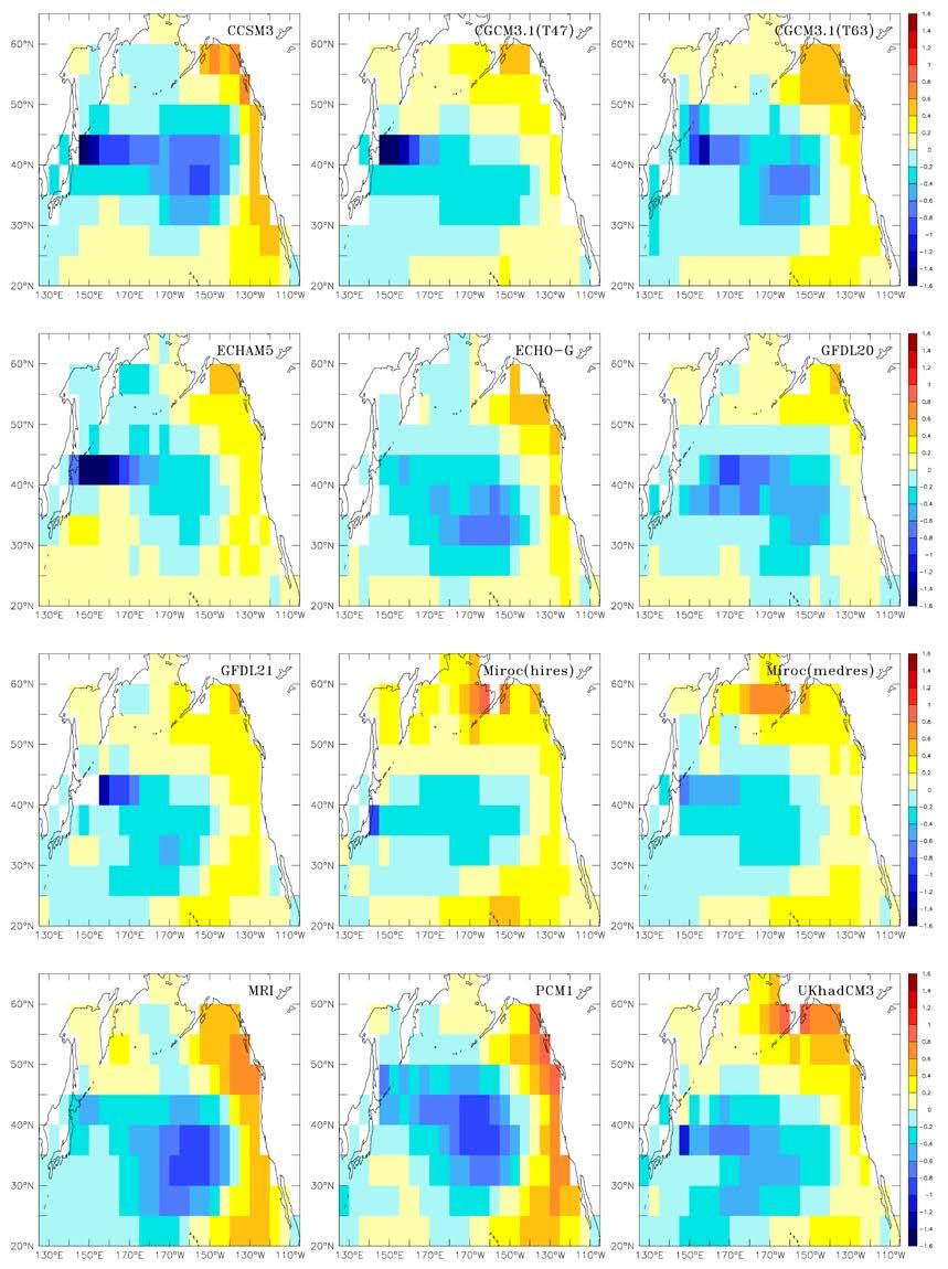
13 Quasi-quantitative Assessment of Global Climate Model Capabilities

14

15

16 Dynamical Modeling Higher trophic levels (Pollock etc.) Secondary Producers (Zooplankton) Primary Producers (Phytoplankton) Nutrients NO 3, NH 4 Physical Forcing (Wind, temp, sun)

17 All models are wrong; some models are useful. -- George Box do we have a useful model?

18 ROMS Physical Oceanography Model Horizontal resolution: ~10km, vertical resolution: 60 layers Computes physical properties i.e. temperature, salinity currents BEST-NPZ model coupled to ROMS at every grid point and time-step

19 DATA MODEL T at M2

20

21 ICE NITRATE ICE ALGAE AMMONIUM NITRATE AMMONIUM Excretion + Respiration SMALL PHYTOPLANKTON LARGE PHYTOPLANKTON IRON WATER MICROZOOPLANKTON SMALL COPEPODS Mortality Predation Egestion LARGE COPEPODS Fast sinking DETRITUS Slow sinking DETRITUS Inexplicit food source BENTHOS EUPHAUSIIDS JELLYFISH BENTHIC FAUNA BENTHIC DETRITUS

22 Model Validation: A Regional Approach regions defined based on bio-phys

23 Model Validation: Data availability Location of nitrate data used: All months, all years

24 Model Validation: Nitrate Similar patterns of variations? Similar amplitude of variations? Is the model accurate? All Months, All Regions More complete ROMS physical model validation in Danielson et al, JGR, 2011

25 Model Validation: Nitrate By Region

26 Observations from Rho, Whitledge and Goering (1997) Model Validation: Primary Production Monthly mean daily primary production: Middle Shelf Observed Observed Simulated Simulated

27 1999 Zooplankon Biomass 2004 Day Microzooplankton Small Copepods Large Copepods Euphausiids E-5 Compares reasonably well to Coyle data but will the fish have enough to eat?

28 Model Predictions:Ecosystem Projections Euphausiid production: Annual average for shelf break A single projection g C m Ensemble of runs will define upper and lower limits of projection Zooplankton biomass: Depth integrated at M2 mooring CCC MA

29 FEAST model for forage species and predators Bioenergetics of feeding, growth, spawning Focus on data-driven functional response between predator and prey Use allometric relationships for rates Diet preferences based on stomach data Movement (towards prey concentrations, away from poor conditions, migration for spawning) Currently includes pollock, cod, and arrowtooth flounder

30

31

32 region Prey Type (proportion in diet) by pollock body length (0-80cm) Diet fitting by region stomachs sampled by pollock length by region amphipods, shrimp 3 size classes of copepod in model summed for fitting

33 Combined BTS+Acoustic survey vs FEAST

34 FEAST age-0 seasonal forage potential and stock-assessment estimate of year-class strength Domain 8 (outer northwest shelf) Age 0 foraging potential Colors: stockassessment year-class strength Blue weakest Red strongest Week of year

35 Final Remarks From present to mid-21st century, climate change is liable to have significant impacts on many marine ecosystems. Open questions: (1) Are the ocean components of global climate models sufficient for climate/ecosystem studies? (2) What is the best way to use existing climate model simulations for regional applications? The output from global climate models (perhaps subject to statistical downscaling) can complement that from vertically-integrated numerical models with full dynamics.

36

37 Comparing empirical versus dynamical models for ecosystems projections What are the strong points of each technique? What are the pitfalls of each technique? What are the likely sources of discrepancies between projections made by these two techniques?