Model Evaluation and SIP Modeling

Transcription

1 Model Evaluation and SIP Modeling Joseph Cassmassi South Coast Air Quality Management District Satellite and Above-Boundary Layer Observations for Air Quality Management Workshop Boulder, CO May 9, 2011

2 SIP Modeling One of the cornerstones of an air quality plan Regional numerical simulations are used to demonstrate future standard attainment of federal NAAQS Identify emissions carrying capacity Evaluate optimal control strategy

3 Boundaries of the South Coast Air Quality Management District and Federal Planning Areas Santa Barbara County San Joaquin Valley Air Basin South Central Coast Air Basin Ventura County Kern County Los Angeles County South Coast Air Basin Orange County San Bernardino County Mojave Desert Air Basin Riverside County South Coast Air Quality Management District SCAQMD Jurisdiction San Diego Air Basin San Diego County Salton Sea Air Basin Imperial County 3 2

4 Plan Summary Inclusive Control Strategy 2015 PM2.5 Attainment 2024 Ozone Attainment 31 - Stationary Source Measures 30 - Mobile Source Measures Emissions Reductions Needed NOx 203 (29%) VOC 59 (11%) SOx 24 (56%) PM (14%) (76%) 116 (22%)

5 Impact of Revisions to Standards EPA will lower 8-hr ozone standard to between ppb (expected end July 2011) Revisions to the annual PM2.5 standard expected to range µg/m3 SCAB surface ozone background simulated at 45 ppb (EPA clean boundaries ppb) Measurement & simulations estimated PM2.5 background at 2-5 µg/m3

6 Challenge Given increasingly more stringent pollutant standards that are closer to background concentrations, where and how can SIP modeling errors be minimized to optimize model performance?

7 SCAQMD Modeling Platforms Meteorological Model MM5 WRF Dispersion Platform CMAQ CAMx Chemistry SAPRC 99 (SAPRC 07) CB-5 One Atmospheric Aerosol PM CAMx

8 Three Nested Domains (New Statewide Domains)

9 Innermost Modeling Domain with Terrain Heights

10 Modeling Considerations Boundary conditions critical to model performance Qualifications of land use, biogenic profiles & soil moisture impact Emissions estimation Wind field generation & stability Insolation Long-range transport impacts both ways From Asia & Mexico Across the U.S. Between air basins

11 Sources of Uncertainty Emissions quantification Temporal and spatial variations Weather impacts Meteorological field development Nested analyses Complex terrain Dispersion analysis Integrating numerical simulations Boundary and initial conditions

12 Emissions and Growth Estimates Biogenic emissions and fugitive dust are dependent upon GIS defined land-use specification Selected inventories are weather adjusted (e.g. biogenic, evaporative emissions) GIS land-use mapping regionally distributes emissions Inventories grown for future years Boundary conditions adjusted to reflect projected emissions control implementation

13 Estimating Emissions Uncertainty Historically estimates of emissions are always subject to the greatest level of uncertainty Methods used to estimate uncertainty Emissions reconciliation through quality assurance and model performance Graphical overlays Model validation requires the inventories be fixed by an agreed date

14 Meteorological Fields Analyses reliant mostly on linked-nested modeling systems Nudging with FDDA Not always productive introduces numerical uncertainty Primary evaluation conducted independent of air quality simulation Fine tuning soil moisture and/or land-use to impact dispersion and wind flow

15 Evaluation of PBL Schemes for a July 2005 Ozone Episode YSU scheme outperformed the other two

16 Extending Domain to Obtain Clean Boundaries Western Boundary Assumptions km offshore Beyond Shipping lanes Limited impacts of recirculation Specify precursor profile Override defaults if data available Upper Air 6 km Ozone 60 ppb (measured, summer)

17 2007 SIP SIP Attainment modeling boundary conditions WRAP CAMx Geochem Regional Haze Model output -- seasonally adjusted & rescaled U.S. EPA s Modified Clean assumption Top boundary from upper air measurements

18

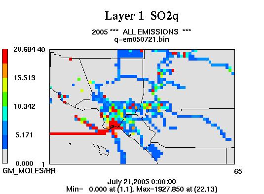
19 Impact of Shipping and Port Activities Ship SOx and NOx emissions contribute heavily to PM2.5 formation Variable distance between land and boundary Ocean-going vessels routinely cross the modeling domain boundary Extending boundary further presents computational issues 4 km grid/ 16 layers

20 WRAP Base Case: Bias µg/m3 5 PPB SO2: Bias µg/m3 10 PPB SO2: Bias µg/m3 10 PPB: SO2 Bias +0.76µg/m3

21 Transport To U.S. Based on field program measurements and computer simulations Current Estimates Episodic : (Events lasting days) - Ozone 4-8 ppb - Fine Dust >1.0 µg/m 3 - Sulfates >1.0 µg/m 3 Projected Long-term Impact (Measured over years) - Ozone 0.5 ± 0.4 ppb/year - Particulates ~ 3% of Asian dust aerosol reaches US Surface ozone trends in air flowing into the United States

22 Impacts to the Basin: Not well defined but research is underway Other than winter, the Basin is located south of the main transport route from Asia Impacts during episodic events are minor compared to Canada and the Northwest US Particulate and ozone transport is strongest in spring out of phase with peak concentrations observed in the Basin Recent studies focus on the Basin > NASA s ARCTAS 2008: Arctic Research of the Composition of the Troposphere from Aircraft and Satellites > NOAA s CalNex 2010 Research at the Nexus of Air Quality and Climate Change (Aircraft, Lidar, Ships)

23 SCAQMD Sponsored Measurements Aloft & Background Monitoring Ozone, particulates, sulfur dioxide, nitrogen dioxide Boundary Layer & Aloft Aircraft & ozonesondes Catalina-island site Update boundary conditions for regional modeling

24 Aircraft Flight Plan

25 Height (m) O3 Profiles for Numerical Modeling 6000 Average Ozone Profiles Ozone (ppb) May-Sep May-Oct Jul-Sep AllYear CMAQ ---- AQMP

26 Layer Num ber Lateral Boundary Values Boundary Value Profile #1 Base Profile O3 (ppb)

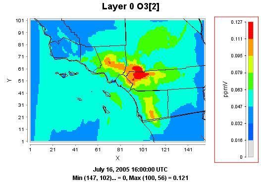
27 O3 Differences in the 1 st layer

28 Max O3 1 st Layer Differences

29 Vertical Cross Section

30 Summary Attainment demonstrations need to account for background concentrations including long-range transport The impact can effect the carrying capacities and hence control strategies Measurements and observations can provide characterization but the extent of data is limited by size of domain and resources Output from global models may have too coarse of grid scale for local application Satellite measurements can fill the void