Air Pollution and Acute Respiratory Infections among

Transcription

1 Air Pollution and Acute Respiratory Infections among Children 0 4 Years of Age: an 18 Year Time Series Study Society of Toxicology Occupational and Public Health Specialty Sections October 30, 2015 Lyndsey Darrow Assistant Professor Department of Epidemiology Rollins School of Public Health Emory University

2 Outline Background and Motivation Methods Results Discussion of design and interpretation issues throughout

3 Study question Are short term changes in outdoor air pollution concentrations associated with counts of emergency department visits for respiratory infections in early life

4 Background Why children 0 4? Lungs developing Respiratory infections commonin early life Differences in lung function and immune system Major reason for emergency health care in this age group Children breathe more air per unit body weight than adults Anatomically smaller peripheral airways Different behaviors that lead to more outdoor air exposures Less research targeting children 0 4, but studies suggest enhanced susceptibility

5 Background Many common respiratory infections in young children possibly exacerbated by air pollution Upper U respiratory infections i Bronchiolitis Bronchitis Lower respiratory infections Pneumonia

6

7 Emergency Department Data For period collected directly from 41 of 42 hospitals in 20 county Atlanta For period, purchased from the Georgia Hospital Association Computerized billing records included Date of visit Primary and secondary ICD diagnosis codes Age

8 Study Area, Hospitals and Population Density

9 Respiratory Diseases of Interest Case groups based on primary ICD 9 codes Bronchiolitis 466.1, , Bronchitis (acute) Pneumonia Upper Respiratory Infection (nasopharyngitis, sinusitis, pharyngitis, tonsillitis, laryngitis, tracheitis, croup, multiple or unspecified site)

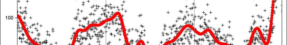
10 ED Visit Counts

11 Air Pollutants of Interest Particulate Matter (PM) PM PM 10 PM 2.5 PM 2.5 species Daily since 1996 Daily since 1998 sulfate (SO 4 ) nitrate (NO 3) ammonium (NH 4 ) elemental carbon (EC) organic carbon (OC) Gases CO (1-hr max) NO 2 (1-hr max) SO 2 (1-hr max) O 3 (8-hr max) Daily since 1993

12 PM composition (by mass) in Atlanta Atlanta PM 2.5 (median mass 16 μg/m 3 ) other metals SO 4 NO 3 OC EC NH 4

13 Time-Series Approach Variation in exposure over time is examined in relation to variation in disease counts A priori lag: 3-day moving average Pollution Date Disease counts Date

14 Design Attributes Not vulnerable to confounding by time invariant risk factors (parental smoking, socio economic status) Vulnerable to confounding by time varying risk factors Long term time trends Generally controlled by including smoothers Risk factors exhibiting short term variation E.g., meteorology controlled in the model

15 Characterizing Daily Ambient Concentrations in the Study Area

16 Characterizing ambient concentrations No. monitors NO 2 6 CO 5 SO O 3 13 PM 10 PM 2.5 PM 2.5 components 9 (2 daily) 13 (9 daily) 6 (4 daily) Networks: EPA s Air Quality System (AQS) Assessment of Spatial Aerosol Composition in Atlanta (ASACA) Southeastern Aerosol Research and Characterization (SEARCH) GOAL: use all available observations to best represent the dil daily ambient levels l of the pollutants in the study area

17 Considerations with spatial averaging of monitors Missing days, monitoring frequency Sometimes use different instruments EC/OC (thermal optical reflectance/remittance) PM 2.5 (FRM vs. TEOM) SO 2 (SEARCH monitors higher due to less loss by condensation) Where in study area do children spend time? Important for spatially heterogeneous pollutants Ideal: time and location weighted ambient pollutant concentrations for each child age 0 4 in the population

18 Population weighted spatial average Normalize log transformed concentrations at each monitor (mean=0, sd=1) Calculate concentration at each of 659 Census tract centroids using the normalized daily dil concentrations ti and inverse distance weighting ihti Convert normalized concentration back to a concentration using a function of distance from urban center to centroid Average the concentrations across Census tracts, weighting by number of people residing in each tract *Ivy et al. Development of ambient air quality population weighted metrics for use in time series health studies. J Air & Waste Manage Assoc 2008; 58:

19 Census tract population data, census tracts 4,112,198 population

20 County Atlanta

21 County Atlanta

22 Epidemiologic Modeling Poisson regression Challenge: control for confounding by time trends and meteorology Meteorological control Moving average lag of maximum temperature (cubic terms) Moving average lag of dew point (cubic terms) Seasonality and longer term trends Cubic splines with 1 knot/month Extensive sensitivity analyses

23

24

25

26

27

28

29 Pollutant effect estimation Linear term for lag moving average Calculate rate ratios for an interquartile range increase in concentration (IQR) More flexible modeling of concentration response using generalized additive models dl (LOESS) Pollutant IQR O ppb CO 0.54 ppm NO ppb SO ppb PM μg/m 3 PM μg/m μg/ PM 2.5 SO μg/m 3 PM 2.5 NO μg/m 3 PM 2.5 NH μg/m/ 3 PM 2.5 EC 0.6 μg/m 3 PM OC 1.7 μg/m 3

30 Negative control exposures Always concerned about confounding in observational studies Possible omitted confounders from model dl Possible confounders misspecified in model (e.g., form of control for meteorology, seasonality and longer term timetrends) trends) Negative control exposures are one of the few tools available to epidemiologists to detect residual confounding Many more tools available for predictive models (e.g., model fit) Lipsitch et al. Negative controls: A tool for detecting confounding and bias in observational studies. Epidemiology 2010; 21:

31 Lag 1 (future) pollution as a negative control We use future concentrations of pollutant as a negative control exposure Meets the definition of a negative control exposure High correlation between today s pollutant level and tomorrow s Future pollution not caused by the outcome (ED visits) Future pollution does not cause today s ED visit (because occurs after) Relies on a central tenet of causality: a cause must precede its effect If tomorrow s pollution is associated with today s disease, after accounting for the relevant past exposures, this must reflect a spurious association Flanders et al. A method for detection of residual confounding in time-series and other observational studies. Epidemiology 2011; 22:

32 Lag 1 (future) )pollution as a negative control Add future (tomorrow s) pollution to our models as an indicator of model problems The effect estimate for future pollution should be null! Any association between the future variable and the outcome must be spurious a) Unmeasured confounding b) Measurement error c) Model misspecification (e.g., misspecification of lag period, dose response, etc.) d) Type 1 error If the future pollutant level is associated with the outcome because the control for the long term or seasonal trends is inadequate then sensitivity analyses can help hl to reveal this

33 Rate Ratios for tomorrow s pollution in relation Rate Ratios for tomorrow s pollution in relation to today s ED visits for URI to today s ED visits for bronchiolitis (age <1)

34 Overall Age Rate Ratio (95% CI) per IQR PNEU UR RI PNEU UR RI PNEU UR RI PNEU UR RI PNEU UR RI PNEU UR RI PNEU UR RI PNEU UR RI PNEU UR RI PNEU UR RI O3 NO2 CO PM10 PM2.5 SO4 NO3 NH4 EC OC

35 atio (95% CI) per IQR Pneumonia Age <1 Age Rate R <1 YR 1 4 YRS <1 YR 1 4 YRS <1 YR 1 4 YRS <1 YR 1 4 YRS <1 YR 1 4 YRS <1 YR 1 4 YRS <1 YR 1 4 YRS <1 YR 1 4 YRS <1 YR 1 4 YRS <1 YR 1 4 YRS O3 NO2 CO PM10 PM2.5 SO4 NO3 NH4 EC OC

36 URI Age <1 Age Rate Ratio (95% CI) per IQR <1 YR 1 4 YRS <1 YR 1 4 YRS <1 YR 1 4 YRS <1 YR 1 4 YRS <1 YR 1 4 YRS <1 YR 1 4 YRS <1 YR 1 4 YRS <1 YR 1 4 YRS <1 YR 1 4 YRS <1 YR 1 4 YRS O3 NO2 CO PM10 PM2.5 SO4 NO3 NH4 EC OC

37 Flexible modeling of concentration response

38 Flexible modeling of concentration response

39 Pneumonia March-October November-February Mean ozone 53 ppb 29 ppb

40 Upper Respiratory Infections March-October November-February

41 Joint Effects Models Many pollutants are correlated, confounding by copollutants is a problem Challenges of multi pollutant models Differences in measurement error by pollutant (e.g., NO 2 vs. O 3 ) Surrogate issue: pollutant is representing an unmeasured, or less well measured, etiologic agent Beta for given pollutant from multi pollutant model may be more or less biased than from single pollutant model Eti Estimate t joint effect of a simultaneous increase in multiple l pollutants t Avoids double counting of pollutant effects from single pollutant models Use multipollutant models to estimate the total effect of IQR increase in all pollutants

42 Joint Effects Results A) PNEU B) URI Ratio Rate Rate Ratio PM 2.5 EC CO NO 2 O 3 EC CO O 3 PM 2. O 3 EC O 3 CO Single Pollutant NO 2 5 Joint Effect Model O 3 11 NO PM 2.5 EC CO NO 2 O EC 3 CO NO 2 Single Pollutant Model O 3 PM O 3 EC 9 O 3 10 CO Joint Effect O 3 11 NO 2 12

43 Summary of Results For pneumonia and upper respiratory infection Evidence of association with ozone, PM organic carbon, and several primary traffic pollutants (CO, NO 2, PM 2.5 EC) Not all independent effects Variation in associations by PM composition strongest for carbon fraction, particularly organic carbon Generally stronger associations for age 1 4 than for infants Highest per unit rate ratios observed for ozone when ozone concentrations lowest

44 Major Strengths and Limitations Strengths Daily PM component data from multiple monitors over 12 years Large numbers of ED visits to investigate these outcomes specifically among young children Use of a negative control exposures and extensive sensitivity analyses Limitations Measurement error in outcomes can be difficult to distinguish i i between respiratory infections, especially in young children Measurement error in exposure spatial heterogeneity of pollutants

45 Estimating concentration response Relationship of outdoor concentrations and ED visits conditional on bh behavioral patterns (e.g., air conditioning i use) Estimating effect of high outdoor air pollution, not necessarily the effect of people breathing high air pollution Accurate estimation of concentration response is of value for setting regulatory standards and maximizing protection of public health

46 Acknowledgments Southeastern Center for Air Pollution & Epidemiology (SCAPE) Coauthors: Mitch Klein, Dana Flanders, Jim Mulholland, Pi Paige Tolbert, Tlb tmtth Matthew Strickland Funding: EPA Clean Air Center RD NIEHS R03ES NIEHS K01ES (MS) R834799

47 View of Atlanta from Stone Mountain. Photo courtesy of Mothers and Others for Clean Air.

48 Extra Slides

49 Negative control exposures Research Question: Does A cause Y? A negative control exposure (B): 1. Is not caused by the disease of interest (Y) 2. Is well correlated with (A) 3. Does not cause (Y) Lipsitch et al. Negative controls: A tool for detecting confounding and bias in observational studies. Epidemiology 2010; 21:

50 Research Question: Does AP 0 cause D 1? Flanders et al. A method for detection of residual confounding in time-series and other observational studies. Epidemiology 2011; 22: