Earth System Modeling at GFDL:

Transcription

1 Earth System Modeling at GFDL: Goals, strategies and early results for the carbon system John Dunne In coordination with researchers at GFDL and PU

2 Background

3 The CO 2 Climate Forcing Question CCSP Strategic Plan, 2003

4 Climate Forcing and Feedbacks CCSP Strategic Plan, 2003

5 The New Fashion: Earth System Modeling As a natural progression of IPCC style assessments, The US Climate Change Science Program s Strategic Plan has called for the next generation of climate simulations to include explicit carbon cycling. This task involves a daunting synthesis of climate models, terrestrial ecology models and ocean biogeochemistry models.

6 Climate Objectives: Simulate the past, present and future climate with dynamic carbon cycles Identify modes of variability and key susceptibilities. Predict biospheric response to human-induced change. Quantify biosphere climate feedbacks Biogeochemical Objective: Identify biospheric and biogeochemical controls Explore relationships between biospheric components Quantify the degree to which the biosphere maintains optimal conditions for itself (i.e. the GAIA hypothesis)

7 Development Application Timeline of Model development CCSP Strategic Plan, 2003

8 Current Challenges The complexity and computational intensity of these models have grown beyond the scope of individual investigators. The large climate modeling centers are all involved in incorporating explicit carbon cycling into their models. This is a monumental task no one group has yet succeeded without making large concessions and dubious assumptions.

9 Centers developing these models Hadley Centre (UK) IPSL (France) NCAR (USA) GFDL (USA) MPI (Germany) JMA-MRI (Japan) CCSR (Japan) CCCMA (Canada) BMRC/CSIRO (Australia) others???

10 Strategy Simulate global elemental cycles within the atm-ocean-land-ice-river system: Carbon (both CO 2 and CH 4 ) Nitrogen Dust/Iron Sulfur Include important biospheric processes effecting climate and feedbacks: Ocean radiative bio-feedbacks through Chlorophyll absorption Ice radiative bio-feedbacks and gas exchange effects Iron transport deposition Eutrophication (anoxia and red tide) Ecological variability and change Atmospheric chemistry and pollution Glacial-interglacial cycles Human activities such as land use, marine resources

11 Schematic of an Earth System Model Climate Model Ocean GCM Atmospheric GCM Land physics and hydrology Earth System Model Atmospheric GCM Tracer transport and chemistry Ocean ecology and biogeochemistry Ocean GCM Dynamic vegetation and land use Land physics and hydrology

12 Current GFDL climate model

13 GFDL Climate Model Description Coupled model referred to as CM2.0 and CM2.1. AM2 atmosphere (2 o horizontal, 24 levels) Version CM2.0 uses b-grid Version CM2.1 uses finite volume grid MOM4 ocean model, 1 o horizontal, 0.3 o at Equator, 50 levels) Sea ice, land, river routing models A complete suite of experiments has been conducted for the IPCC 2007 report. Detailed descriptions of these models available at: Model output available at:

14 Model SST Errors CM2.0 CM2.1 Courtesy of Tom Delworth

15 Courtesy of Tom Delworth

16 CM2.1 ocean sensitivity to forcing CO 2 from solubility (Pg) Courtesy of Tom Delworth

17 GFDL Ocean Biogeochemistry Description

18 Ocean Biogeochemical Model Carbon Oxygen Phosphorus Dissolved organic matter cycling Particle sinking and respiration Air-Sea gas flux Nitrogen Iron SiO 2 and CaCO 3 Solubility pump Deposition Mineral pump Loss from system

19 Ocean Ecosystem Model N 2 -fix. Phyto. Fish Recycled nutrients New Nutrients Small Phyto. Protists Filter Feeder DOM Large Phyto. Detritus

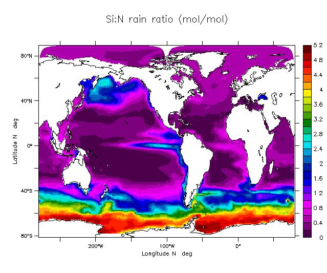
20 Uptake Components N-uptake is based on Geider et al. (1997), except for the treatment of iron: Q Fe:N = Fe:N 2 / (Fe:N lim + Fe:N 2 ) φ = φ max /(1 + φ max α I z / (2 P C m )) Q Fe:N µ N = P C m / (1 + z) (1 exp(-αi z φ/pc m )) Fe-uptake is proportional to dissolved Fe: Uptake Fe = V Fe Lim Fe exp(kt) P N (1 Q Fe:N ) Model fit to Sunda and Huntsman (1997) for T. Pseudonana under high (open) and low light (filled): Diazotrophs have slow growth and high N:P. The Si:N uptake ratio is: Si:N = (Si:N max Si:N min )Si:N lim /(Si:N max + Si:N lim ) + Si:N min CaCO 3 production is a fraction of small Phytoplankton production. Si:N of diatom uptake Lim Si /min(lim Irr/Fe, Lim N, Lim P )

21 Recycling Components Grazing of P S P S 2 Grazing of P L and P Di P 4/3 Detritus production a function of P S,P L, and P Di grazing and T Grazing threshold prevents phytoplankton extinction Dissolved Fe adsorbs onto sinking organic particles Sinking detritus protected from remineralization by mineral after Klaas and Archer (2002) Semilabile DON (t remin = 18 yr), Semilabile DOP (t remin = 4 yr; Abell et al., 2000), and Labile DOM (t remin = 3 mo) produced as constant fractions of grazing.

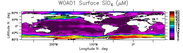
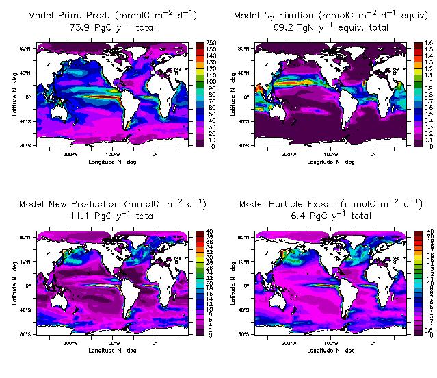
22 GFDL Ocean Biogeochemistry Results (NCAR/NCEP Reanalysis)

23

24

25

26

27

28

29

30

31 Global variability in Nitrogen Cycling Tg N yr -1 Water Column Denitrification N 2 Fixation Sediment Denitrification % Percent of anoxic waters (by volume)

32

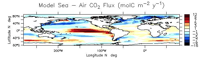
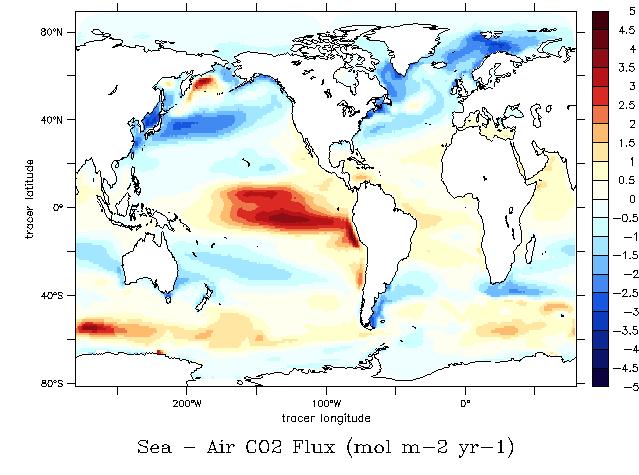
33 Pg C yr -1 Global Sea-Air CO 2 Flux

34 Global Sea-Air CO 2 Flux Variability

35 Summary of reanalysis results Large scale WOA01 and SeaWiFS patterns are reproduced though the Southern Ocean is too low in surface nutrients. Many areas of improvement remain: Eq. Pacific HNLC region larger than observations Eq. Pacific chlorophyll and production also in excess. North Atlantic subtropical gyre is too far south North Atlantic spring bloom terminates too early Global Sea-Air variability in CO 2 fluxes consistent with expectations from radiative forcing Intermittently ice-covered regions do not out-gas significant levels of CO 2 in this model. Water column denitrification varies significantly on inter-annual time-scales.

36 Current Challenges

37 Practical development issues Model Complexity: Composed of 10 6 lines of code and scripts Includes 10 3 parameter options Includes 10 2 restart and initialization files Written by people Incomplete documentation Code is constantly changing Model speed: Code retrieval and compilation takes 3 hours Input retrieval for short runs takes up to 2 hours Model runs 6 years per day on 126 processors Output retrieval of model year takes 2 hours Computer system glitches increase time by Model size: Monthly output for a model year is 16Gb

38 How to initialize the carbon system? Fossil Fuels Atmosphere 560 PgC (280 ppmv) + FF ~90 PgC ~60 PgC Turnover Time ~4 yr Turnover Time yr Ocean BGC Land BGC Pg C + FF 2000 Pg C Turnover Time yr equilibrium takes yrs running 1000 years takes >6 months

39 Options to initialize the carbon system Run the model out for a very long time Perform short runs with drift and always reference to a control Run until the drift becomes small relative to the anthropogenic increase Run until the drift becomes smaller than the natural variability Accelerate the carbon system towards equilibrium Correction via drift extrapolation Inverse methods Correction via solubility and biological pump separation

40 Is a steady state ever achieved? Short term solar and volcanic forcings vary on the order of 5W m -2 : CO 2 solubility variability 1 Pg C yr -1 Long term radiative budget has ~1W m -2 heat uptake in standard climate run: CO 2 solubility outgassing 2 Pg C decade -1 Nitrogen cycle has long time-scale variability

41 When is the model good enough? Is the model constructed robustly? Nitrate, Silicate and Fe at mode water formation Timing of blooms relative to sea ice cover How does one assess model fidelity? Cruise data is sparse, both temporally and geographically Data information can seem contradictory What to do when biospheric dynamics degrades climate? Example: Current run turns the Amazon to a desert.

42 When is the model good enough? Analogy with GFDL s CM2 development : SST < 10 C away from Levitus NADW > 10 Sv El Nino (1 yr < trop. osc. < 5yr) Examples of ESM options: Control run dco 2atm /dt less than 2 Pg C/decade? Vegetation type (Rainforest/desert/savanna/etc) agreement with observations? Surface nutrient agreement with observations? Surface CO 2 flux agreement with observations? Land NPP, Ocean NPP? Others?

43 Which processes must be simulated? Physical pathways are simplified e.g. no explicit rivers, estuaries or sediments. Are these neglected processes important to CO 2 radiative feedbacks? Biogeochemistry has long time scales that cannot be simulated. What do we need to know about longer timescales? How is our lack of information affecting our understanding? Biology is far more complex than we can simulate computationally. What susceptibilities need to be represented?

44 Can the Earth be modeled as a single system, or do different goals require different models? Hard: Climate goals only require processes with climate feedbacks: Importance defined radiatively in W m -2 Land albedo, transpiration and CO 2 exchange Ocean CO 2 exchange (and perhaps Chl) CH 4 cycle? Harder: Biogeochemical goals require ecosystem complexity: Terrestrial Ecology Ocean Ecosystems Rivers, sediments, sea ice Hardest: Human impact goals require getting all the rest right: Human health Water supplies Agriculture Fisheries Susceptibility to Catastrophe

45 How to address ecologically-forced degradation in physical simulation? Until very recently, global climate models had to an artificial flux adjustment at the air-sea interface to keep the climate stable and representative What types ESM tunings are advisable? Should CO 2 fluxes be adjusted to reproduce atmospheric concentrations over time? Should ecological feedbacks be tuned to compensate for poor-physics (Amazon example).

46 Short-term Earth System Modeling Plans Code synchronization with climate group Address current issue of Amazon fidelity degradation Spinup to quasi steady state. Run IPCC scenarios of to quantify: Ecosystem feedbacks on atmospheric CO 2 Climate feedbacks on ecosystems Assess CO 2 fluxes under various CO 2 emissions, land use and mitigation scenarios.

47 Long-term Earth System Modeling Plans FY2004 FY FY FY Application 2º Atmosphere Atmos. Physics Land Model 1º Ocean Model SIS Sea Ice Model Common Infrastructure 2º Atmosphere Atmos. Physics LM3 Land Model 1º Ocean Model SIS Sea Ice Model Full Carbon Cycle ½º Atmosphere Atmos. Physics Land Model ¼º HC Ocean Model SIS Sea Ice Model Full C, N, and P Cycles 10km Atmosphere Atmos. Physics Land Model Sea and Land Ice Model 1/10º HC Ocean Model SIS Sea Ice Model CM2 Interactive Chemistry Common Infrastructure Interactive Chemistry NOAA-ESMF Infrastructure Full Biogeochemical Cycles Interactive Chemistry NOAA-ESMF Infrastructure Development Ocean N,P cycles Full Carbon Cycle Interactive Chemistry LM3 Land Model IPCC scenarios Climate datasets Regional projections NOAA-ESMF Infrastructure ¼º HC Ocean Model Cont. Shelf Model Terr. N, P Cycles ½-¼º Atmosphere Land Ice Model CCTP if-then scenarios 1/6-1/10º Ocean Model 1/20-1/50º Ocean Model Additional Chem. Cycles 10km NonH Atmosphere Land Ice Model IPCC scenarios > 1000X in computation Additional Chem. Cycles 1km NonH Atmosphere Ecosystems forecasts Extreme events Role of short-lived species Decadal projections Detection and attribution Climate of the 20 th Century

48 How can data improve models? Provide boundary and initial conditions WOCE, NCEP, GLODAP, etc. Data synthesis => Improved theory => implementation Effect of mineral on organic flux Data - Model comparison => flaws in models => refutation of model => new theory => implementation HNLC EqPac - IronEx I IronEx II Fe in models