Micro-power System Modeling using HOMER - Tutorial 1

Transcription

1 Micro-power System Modeling using HOMER - Tutorial 1 Charles Kim Howard University 1

2 HOMER Homer (Hybrid Optimization Model for Electric Renewables) 2

3 Homer a tool A tool for designing micropower systems Village power systems Stand-alone applications and Hybrid Systems Micro grid 3

4 HOMER Legacy software 4

5 Homer - capabilities Finds combination components that can service a load at the lowest cost with answering the following questions: Should I buy a wind turbine, PV array, or both? Will my design meet growing demand? How big should my battery bank be? What if the fuel price changes? How should I operate my system? And many others

6 Homer - Features Simulation Estimate the cost and determine the feasibility of a system design over the 8760 hours in a year Optimization Simulate each system configuration and display list of systems sorted by net present cost (NPC) Life-Cycle Cost: Initial cost purchases and installation Cost of owning and O&M and replacement NPC: Life-cycle cost expressed as a lump sum in today s dollars Sensitivity Analysis Perform an optimization for each sensitivity variable 6

7 Features Homer can accept max 3 generators Fossil Fuels Biofuels Cogeneration Renewable Technologies Solar PV Wind Biomass and biofuels Hydro 7

8 Features Emerging Technologies Fuel Cells Microturbines Small Modular biomass Grid Connected System Rate Schedule, Net metering, and Demand Charges Grid Extension Breakeven grid extension distance: minimum distance between system and grid that is economically feasible 8

9 Loads Electrical Thermal Hydrogen Resources Features Wind speed (m/s) Solar radiation (kwh/m 2 /day) Stream Flow (L/s) Fuel price ($/L) 9

10 Optimization Best possible system configuration that satisfies the user-specified constraints at the lowest total NPC (net present cost). Decide on the mix of components that the system should contain, the size or quantity of each component, Ranks the feasible ones according to total net present cost 10

11 Optimization Example Configuration and 140 (5x1x7x4=140) search spaces Overall Optimization results Categorized optimization result 11

12 Sensitivity Analysis Optimization: best configuration under a particular set of input assumptions Sensitivity Analysis: Multiple optimizations each using a different set of input assumptions How sensitive the outputs are to changes in the inputs results in various tabular and graphic formats User enters a range of values for a single input variable: Grid power price Fuel price, Interest rate Lifetime of PV array Solar Radiation Wind Speed 12

13 Why Sensitivity Analysis? Uncertainty! When unsure of a particular variable, enter several values covering the likely range and see how the results vary across the range. Diesel Generator Wind Configuration: Uncertainty in diesel fuel price with $0.6 per liter in the planning stage and 30 year generator lifetime Example: Spider Graph Tabular Format 13

14 Sensitivity Analysis on Hourly Data Sets Sensitivity analysis on hourly data sets such as primary electric load, solar/wind resource 8760 values that have a certain average value with scaling variables Example: Graphical Illustration Hourly primary load data with an annual average of 22 kwh/day with average wind speed of 4 m/s Primary load scaling variables of 20, 40, ---, 120kWh/day & 3, 4, ---, 7 m/s wind speeds. 14

15 Resources Modeling Solar Resources: average global solar radiation on horizontal surface (kwh/m 2 or kwh/m 2 -day) or monthly average clearness index (atmosphere vs. earth surface). Inputs solar radiation values and the latitude and the longitude. Output 8760 hour data set Wind Resources: Hourly or 12 monthly average wind speeds. Anemometer height. Wind turbine hub height. Elevation of the site. Hydro Resources: Run-of-river hydro turbine. Hourly (or monthly average) stream flow data. Biomass Resources: wood waste, agricultural residue, animal waste, energy crops. Liquid or gaseous fuel. Fuel: density, lower heating value, carbon content, sulfur content. Price and consumption limits 15

16 Component Modeling See Appendix for details HOMER models 10 types of part that generates, delivers, converts, or stores energy 3 intermittent renewable resources: PV modules (dc) wind turbines (dc or ac) run-of-river hydro turbines (dc or ac) 3 dispatchable energy sources: [control them as needed] Generators the grid boilers 2 energy converters: Converters (dc ac) Electrolyzers (ac,dc electrolysis Hydrogen) 2 types of energy storage: batteries (dc) hydrogen storage tanks 16

17 1. Collect Information How to build a HOMER project Electric demand (load) Energy resources 2. Define Options (Gen, Grid, etc) 3. Enter Load Data 4. Enter Resource Data 5. Enter Component Sizes and Costs 6. Enter Sensitivity Variable Values 7. Calculate Results 8. Examine Results Caveat: HOMER is only a model. HOMER does not provide "the right answer" to questions. It does help you consider important factors, and evaluate and compare options. 17

18 Load profile: Example Case Micro Grid in Sri Lanka base load of 5W, small peaks of 20 W, peak load of 40W; total daily average load = 350 Wh Sensitivity analysis range: [0.3kW/h, 16kWh/d] Solar Resource 7.30 Latitude & longitude NASA Surface Meteorology and Solar Energy Web: average solar radiation = 5.43 kwh/m 2 /d. Economics: Real annual interest rate at 6% $0.4/L $0.7/L Reliability Constraints Sensitivity analysis range: [$0.3, 0% annual capacity shortage 0.8] with increment of $0.1/L Sensitivity Analysis range: [ ]% Diesel Fuel Price

19 Example Case Micro Grid in Sri Lanka PV: de-rating factor at 90% Battery:T-105 or L-16 Converters: efficiency at 90% for inversion and 85% for rectification Generator: not allowed to operate at less than 30% capacity 19

20 Analysis Result Diesel price $0.3/L Diesel Price $0.8/L 20

21 HOMER: Getting Started with existing file 1. ExampleProject.hmr 2. Open the Example Project File: ExampleProject.hmr 3. Click the Primary Load 4. Exit out of HOMER We have things to do 21

22 Latitude and Longitude Find the Site [Location] Your dorm room Your home Your favorite place 22

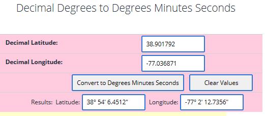
23 LAT and LONG --- Conversion 23

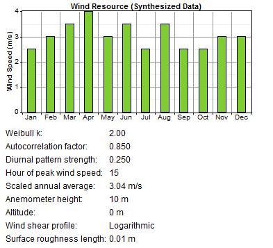
24 Resources Average Monthly Irradiation and Wind Speed 24

25 MASA 25

26 Next Step 26

27 Select Parameters Just 2 below are enough 27

28 Monthly Data for Insolation and Wind Speed 28

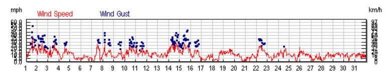
29 Sources for Wind Data 29

30 Click the generator HOMER: Open the file again 25 kw $10,000 Minimum running at 30% 30

31 Click Wind Turbine Equipment From the drop down list click through the wind turbines and look at the power curve. Try to find a Wind Turbine that would best maximize Average Wind Speed (m/s) :

32 Click PV Equipment Lifetime, De-rating factor, slope, No-tracking 32

33 Resource Information Select Solar Resources, Wind Resources, and Diesel Type in Solar Radiation Type in Wind Speed Diesel Fuel Price 33

34 Click Converter icon 5kW $4,000 Equipment 34

35 Economics Real interest 6 % Lifetime 25 years System Control Cycle-charging Other Information 35

36 Emission: all 0 This time Constraints Operating reserve 10% Capacity shortage 0% Other Information 36

37 Emission Calculation in HOMER Carbon content of fuel If CO 2 is only interest Set 0 to CO Set 0 to UHC 37

38 Fuel Carbon Content Diesel Natural Gas Gasoline 38

39 Carbon Tax or Penalty Carbon penalty will appear as Other O&M Cost. 39

40 Example 3 Generators only to meet a load Diesel generator Carbon 88% of 820 kg per 1000 L Gasoline generator Carbon 86% of 740 kg per 1000L Natural Gas generator Carbon 67% of 0.79kg per 1 m 3 Total fuel consumption for each Diesel 10,996 L Gasoline 1,762 L Natural Gas 2,613 m 3 Carbon Content Diesel: 820 * * 0.88 = 7974 kg/yr Gasoline: 740 * * 0.86 = 1,121 kg/yr Natural Gas: 0.79 * 2,613 * 0.67 = 1,383 kg/yr Total = 10,478 kg/yr Total CO 2 10,478 kg * 3.67 = kg CO 2 /year Added O&M Cost per year with $2 per ton of CO 2 $2* = $76.9/yr 40

41 System Report - Example 41

42 Emission Input Emission Penalty 42

43 Analysis of the System 1. Click Calculate to start the analysis Click Overall: view all possible combinations 43

44 Click Categorized Analysis of the System Now back to Overall, and choose any system of interest by clicking/ double clicking 44

45 Simulation Results Analysis 45

46 PV Output 46

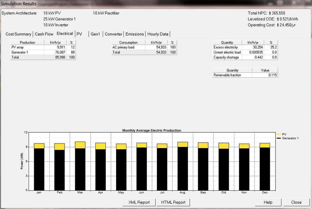
47 Electrical Output 47

48 Sensitivity Analysis on Wind Power Click Wind resource Click Edit Sensitivity Values >> Do so for Load, Solar, and Diesel Wind Resources Primary Load Solar Resources Diesel Fuel 48

49 Save and Calculate New we see the tab for Sensitivity Results Sensitivity Analysis 49

50 HOMER Input Summary Report HOMER Produces An Input Summary Report: Click HTML Input Summary from the File menu, or click the toolbar button: HOMER will create an HTML-format report summarizing all the relevant inputs, and display it in a browser. From the browser, you can save or print the report, or copy it to the clipboard so that you can paste it into a word processor or spreadsheet program. 50

51 Input summary Report - Example 51

52 HOMER Simulation Result System Report HOMER Produces A Report Summarizing The Simulation Results Just click the HTML Report button in the Simulation Results window: 52

53 Example System Report 53

54 System Report 54

55 This message? HOMER displays a message suggesting that we add more generator quantities to the sizes to consider. 55

56 Other messages to appear Those messages mean that: you need to expand your search space to be sure you have found the cheapest system configuration. If the total net present cost varied with the PV size in this way, and you simulated 10, 20, 30, and 40 kw sizes, HOMER would notice that the optimal number of turbines is 40 kw, but since that was as far as you let it look, it would give you the "search space may be insufficient" warning because 50 kw may be better yet. It doesn't know that until you let it try 50kW and 60kW. If you expanded the search space, HOMER would no longer give you that warning, since the price started to go up so you have probably identified the true least-cost point. 56

57 Report Submission for Lab 9 Using the Homer Tutorial Part 1 Follow every step from slide page 21 With your own location Resources are determined With your own loading condition Write your report describing Location, Load, Solar Resources Wind Resources Optimum result (the Price of energy. $/kwh)? Comment and Opinion Appendix 1: Input report from HOMER Appendix 2: Output Report from HOMER 57

58 APPENDIX Physical Modeling - Components HOMER models 10 types of part that generates, delivers, converts, or stores energy 3 intermittent renewable resources: PV modules (dc) wind turbines (dc or ac) run-of-river hydro turbines (dc or ac) 3 dispatchable energy sources: [control them as needed] Generators the grid boilers 2 energy converters: Converters (dc ac) Electrolyzers (ac,dc electrolysis Hydrogen) 2 types of energy storage: batteries (dc) hydrogen storage tanks 58

59 Physical Modeling - load Load: a demand for electric or thermal energy 3 types of loads Primary load: electric demand that must be served according to a particular schedule When a customer switches on, the system must supply electricity kw for each hour of the load Lights, radio, TV, appliances, computers, Deferrable load: electric demand that can be served at any time within a certain time span Tank drain concept Water pumps, ice makers, battery-charging station Thermal load: demand for heat Supply from boiler or waste heat recovered from a generator Resistive heating using excess electricity 59

60 Physical Modeling - Resources Solar Resources: average global solar radiation on horizontal surface (kwh/m 2 or kwh/m 2 -day) or monthly average clearness index (atmosphere vs. earth surface). Inputs solar radiation values and the latitude and the longitude. Output 8760 hour data set Wind Resources: Hourly or 12 monthly average wind speeds. Anemometer height. Wind turbine hub height. Elevation of the site. Hydro Resources: Run-of-river hydro turbine. Hourly (or monthly average) stream flow data. Biomass Resources: wood waste, agricultural residue, animal waste, energy crops. Liquid or gaseous fuel. Fuel: density, lower heating value, carbon content, sulfur content. Price and consumption limits 60

61 PV Array Components- PV, Wind, and Hydro f PV : PV de-rating factor Y PV : Rated Capacity [kw] I T : Global Solar Radiation incidence on the surface of the PV array [kw/m 2 ] I S : Standard amount of radiation, 1 kw/m 2. Wind Turbine Wind turbine power curve Hydro Turbine Power Output Eqn = Turbine efficiency, density of water, gravitational acceleration, net head, flow rate through the turbine 61

62 Generators Components - Generator Principal properties: max and min electrical power output, expected lifetime, type of fuel, fuel curve Fuel curve: quantity of fuel consumed to produce certain amount of electrical power. Straight line is assumed. Fuel Consumption (F) [L/h], [m 3 /h], or [kg/h]: F o - fuel curve intercept coefficient [L/h-kW]; F 1 - fuel curve slope [L/h-kW]; Y gen - rated capacity [kw]; P gen - electrical output [kw] 62

63 Components - Generator Generator costs: initial capital cost, replacement cost, and annual O&M cost per operating hour (not including fuel cost) Fixed cost: cost per hour of simply running the generator without producing any electricity Marginal cost: additional cost per kwh of producing electricity from the generator 63

64 Battery Bank Principal properties: Components Battery Bank nominal voltage capacity curve: discharge capacity in AH vs. discharge current in A lifetime curve: number of discharge-charge cycles vs. cycle depth minimum state of charge: State of charge below which must not be discharges to avoid permanent damage round-trip efficiency: percentage of energy going in to that can be drawn back out Example capacity curve for a deep-cycle US-250 battery (Left) 64

65 Grid and Grid Power Cost Components - Grid Grid power price [$/kwh]: charges for energy purchase from grid Demand rate [$/kw/month]: peak grid demand Sellback rate [$/kwh]: price the utility pays for the power sold to grid Net Metering: a billing arrangement whereby the utility charges the customer based on the net grid purchases (purchases minus sales) over the billing period. Purchase > sales: consumer pays the utility an amount equal to the net grid purchases times the grid power cost. sales > purchases: the utility pays the consumer an amount equal to the net grid sales (sales minus purchases) times the sellback rate, which is typically less than the grid power price, and often zero. Grid fixed cost: $0 Grid marginal cost: current grid power price plus any cost resulting from 65 emissions penalties.

66 Boiler Components - Boiler Assumed to provide unlimited amount of thermal energy on demand Input: type of fuel, boiler efficiency, emission Fixed cost: $0 Marginal cost: 66

67 Converter Components Converter Inversion and Rectification Size: max amount of power it delivers Synchronization ability: parallel run with grid Efficiency Cost: capital, replacement, o&m, lifetime 67

68 Electrolyzer: Components Fuel Cell Size: max electrical input Min load ratio: the minimum power input at which it can operate, expressed as a percentage of its maximum power input. Cost: capital, replacement, o&m, lifetime Hydrogen Tank Size: mass of hydrogen it can contain Cost: capital, replacement, o&m, lifetime 68

69 System Dispatch Dispatachable and non-dispatchable power sources Dispatchable source: provides operating capacity in an amount equal to the maximum amount of power it could produce at a moment s notice. Generator In operation: dispatchable opr capacity = rated capacity non-operation: dispatchable opr capacity = 0 Grid: dispatchable opr capacity = max grid demand Battery: dispatachable opr capacity = current max discharge power Non-dispatchable source Operating capacity (PV, Wind, or Hydro) = the amount the source is currently producing (Not the max amount it can produce) NOTE: If a system is ever unable to supply the required amount of load plus operating reserve, HOMER records the shortfall as capacity shortage. HOMER calculates the total amount of such shortages over the year and divides the total annual capacity shortage by the total annual electric load. 69

70 Dispatch Strategy for a system with Gen and Battery Dispatch Strategy Whether and how the generator should charge the battery bank? HOMER provides 2 simple strategies and lets user model them both to see which is better in any particular situation. Load-following: a generator produces only enough power to serve the load, and does not charge the battery bank. Cycle-Charging: whenever a generator operates, it runs at its maximum rated capacity and charges the battery bank with the excess It was found that over a wide range of conditions, the better of these two simple strategies is virtually as cost-effective as the ideal predictive strategy. Set-point state charge : in the cycle-charging strategy, generator charges until the battery reaches the set-point state of charge. 70

71 Control of Dispatchable System Components Fundamental principle: cost minimization fixed cost and marginal cost Example: Hydro-Diesel-Battery System Dispatachable sources: diesel generator [80kW] and battery [40kW] If net load is negative: excess power charges battery If net load is positive: operate diesel OR discharge battery 71

72 Dispatch Control Example Hydro-Diesel-Battery System Net load < 20kW: Discharge the battery Net load > 20kW: Operate the diesel generator 72

73 Load Priority Decisions on allocating electricity Presence of ac and dc buses Electricity produced on one bus will serve First, primary load on the same bus Then, primary load on the opposite bus Then, deferrable load on the same bus Then, charge battery bank Then, sells to grid Then, electrolyzer Then, dump load 73

74 Economic Modeling Conventional sources: low capital and high operating costs Renewable sources: high initial capital and low operating costs Life-cycle costs= capital + operating costs HOMER uses NPC for life-cycle cost NPC is the opposite of NPV (Net present value) NPC includes: initial construction, component replacements, maintenance, fuel, cost of buying grid, penalties, and revenues (selling power to grid + salvage value at the end of the project lifetime) 74

75 Real Cost All price escalates at the same rate over the lifetime Inflation can be factored out of analysis by using the real (inflation-adjusted) interest rate (rather than nominal interest rate) when discounting the future cash flows to the present Real interest rate = nominal interest rate inflation rate Real cost in terms of constant dollars 75

76 NPC and COE Total NPC Levelized Cost of Energy (COE): average cost/kwh 76