CHARACTERIZING AND IMPROVING PRODUCTION OF FERMENTABLE SUGARS AND CO-PRODUCTS FROM A FOREST PRODUCT INDUSTRY WASTEWATER STREAM

Transcription

1 Michigan Technological University Digital Michigan Tech Dissertations, Master's Theses and Master's Reports - Open Dissertations, Master's Theses and Master's Reports 2014 CHARACTERIZING AND IMPROVING PRODUCTION OF FERMENTABLE SUGARS AND CO-PRODUCTS FROM A FOREST PRODUCT INDUSTRY WASTEWATER STREAM Jifei Liu Michigan Technological University Copyright 2014 Jifei Liu Recommended Citation Liu, Jifei, "CHARACTERIZING AND IMPROVING PRODUCTION OF FERMENTABLE SUGARS AND CO-PRODUCTS FROM A FOREST PRODUCT INDUSTRY WASTEWATER STREAM", Dissertation, Michigan Technological University, Follow this and additional works at: Part of the Chemical Engineering Commons, Environmental Engineering Commons, and the Oil, Gas, and Energy Commons

2 CHARACTERIZING AND IMPROVING PRODUCTION OF FERMENTABLE SUGARS AND CO-PRODUCTS FROM A FOREST PRODUCT INDUSTRY WASTEWATER STREAM By Jifei Liu A DISSERTATION Submitted in partial fulfillment of the requirements for the degree of DOCTOR OF PHILOSOPHY In Chemical Engineering MICHIGAN TECHNOLOGICAL UNIVERSITY Jifei Liu

3

4 This dissertation has been approved in partial fulfillment of the requirements for the Degree of DOCTOR OF PHILOSOPHY in Chemical Engineering Department of Chemical Engineering Dissertation Advisor: David R. Shonnard Committee Member: Susan T. Bagley Committee Member: Tony N. Rogers Committee Member: Wen Zhou Department Chair: S. Komar Kawatra

5

6 Table of Contents List of Tables... ix List of Figures... xi Acknowledgements... xvii Preface... xix List of publications... xxi Abstract... xxiii Introduction and Research Objectives Introduction Dissertation objectives... 4 Chapter 1 Literature Review for the Research Conducted in Chapter 2, 3 and Introduction to feedstock types for biofuels Biomass material characterization Lignocellulosic biomass conversion processes Thermochemical conversion Biochemical conversion Introduction to fermentation inhibitors Furfural and HMF Phenolic compounds Weak acids Life cycle assessment References Chapter 2 Characterization of a Hardboard Manufacturing Process Wastewater Stream and its Suitability for Conversion to Ethanol and Other Co-products Abstract Introduction Introduction to biomass feedstocks, conversion, and characterization Introduction to biomass characterization Research objectives Feedstock and process description Research methods v

7 3.1. Sample preparation for drying, imaging, and filtration Determination of total solid, ash, lignin and carbohydrates Surface structure study using SEM Functional group changes with conversion Elemental analysis Results and discussion Total solid, ash, lignin and carbohydrates Summative mass closure Scanning electron microscopy (SEM) Fourier transform infrared spectroscopy (FTIR) Elemental analysis of solids Conclusion Acknowledgements References Appendix A Documentation for Fair use of Figures 2.2, 2.3 and Chapter 3 Determination of Optimum Hydrolysis Conditions for Conversion of a Forest Product Wastewater Effluent to Fermentable Sugars Abstract Introduction Materials and method Composition of the effluent waste materials Acid pretreatment and enzymatic hydrolysis condition Concentration analysis Statistical analysis Results and discussion Sugar and inhibitory compounds generated during acid pretreatment Sugar yield after enzymatic hydrolysis Statistical Analysis Conclusion Acknowledgements References Appendix B Acid Pretreatment (AP) Results vi

8 2. Enzymatic Hydrolysis (EH) Results Statistical Analysis Results Chapter 4 Life Cycle Carbon Footprint of Ethanol and Potassium Acetate Produced from a Forest Product Wastewater Stream by a Co-located Biorefinery Abstract Introduction Methodology Goal, scope and functional unit definition Description of the process Inputs and inventory for the basecase life cycle carbon footprint Allocation methods Impact Assessment Scenarios Results and Discussion Basecase: Ethanol Basecase: KAc Scenario analyses Future work Conclusion Acknowledgments Associated Content References Supporting Information (SI) for Life Cycle Carbon Footprint of Ethanol and Potassium Acetate Produced from a Forest Product Wastewater Stream by a Co-located Biorefinery Appendix C Permission to Republish Chapter 4 Life Cycle Carbon Footprint of Ethanol and Potassium Acetate Produced from a Forest Product Wastewater Stream by a Co-located Biorefinery Chapter 5 Limitations and Future Work Chapter 6 Conclusions vii

9

10 List of Tables Table 2.1. Characterization methods and experiment tasks...51 Table 2.2. Main functional groups for FTIR...52 Table 2.3. Total Solid and Ash Results...53 Table 2.4. Lignin analysis results...54 Table 2.5. Concentration of important components in pre and post dilute acid pretreatment liquid samples...55 Table 2.6. Mass balance calculation...56 Table 2.7. Amount of each element detected in ppm and % of the solid digested (1 experiment)...57 Table 3.1. Experimental matrix regarding acid pretreatment and enzymatic hydrolysis proceeded (The temperature of the experiments were all conducted at 121 o C)...90 Table 3.2. High and low enzyme dosage in enzymatic hydrolysis...91 Table 3.3a. Responses Obtained under different acid pretreatment conditions. The unit of yield is expressed as (g/l monomer sugars or total sugar)/(77.03g/ l total solid) Table 3.3b. Responses Obtained under different acid pretreatment conditions, the unit of yield is expressed as (g/l inhibitors)/(77.03g/l total solid) Table 3.4. Optimum condition and ANOVA analysis results after acid pretreatment. The unit of yield is expressed as (g/l monomer sugars or total sugar)/ (77.03g/l total solid) Table 3.5. Regression model responses obtained under different hydrolysis conditions. The unit of yield is expressed as (g/l monomer sugars or total sugar)/ (77.03g/l total solid) Table 3.6. Optimum condition and ANOVA analysis results after hydrolysis. The unit of yield is expressed as (g/l monomer sugars or total sugar)/(77.03g/ l total solid) Table 3.7. Predicted results of enzymatic hydrolysis from the regression model for total sugar yield. The unit of yield is expressed as (g/l monomer sugars or total sugar)/(77.03g/l total solid) Table 4.1. Inputs, Outputs, and Energy Savings (based on annual operation of a colocated biorefinery in MI) ix

11 Table 4.2. Scenarios for life cycle carbon footprint Model Assumption Uncertainty Table S1. Michigan Grid Distribution Table S2. Distribution of Renewable Power in Michigan Grid Table S3. Inputs and Outputs: Inventory Data with Sources Table S4. GHG Emission from Industrial water Table S5. Mass Allocation Factor Calculation Table S6. Price of Potassium Acetate and Price Fluctuation Estimate Table S7. Market Value (Price) Allocation Factor Calculation Table S8. Ecoprofiles of Alternative Energy Resources in Scenarios 1& Table S9. Scenario Analysis-GHG impact of ethanol from different stages in system expansion method Table S10. Scenario Analysis-GHG impact of ethanol from different stages in market value allocation method Table S11. Scenario Analysis-GHG impact of KAC from different stages in market value allocation method x

12 List of Figures Figure I.1 Mandates set by Energy Policy Act of 2005 and Energy Independence and security Act of Figure 1.1 Biochemical conversion processing...12 Figure 2.1 Process flow diagram for conversion of forest product industry wastewater effluent into biofuel and an acetate-based road de-icer compound Figure 2.2 Cellulose structure (Sigma-Aldrich ( egion=us))...59 Figure 2.3 Lignin structure (Sigma-Aldrich ( egion=us))...60 Figure 2.4 Polymer of -(1-4)-D-xylopyranosyl units (Sigma-Aldrich ( Figure 2.5 Surface structure of three samples with increasing magnification; Solid, Imaging from Table 2.1 is (a-g), Solid, Imaging from Table 2.1 is (h-n), Solid, Imaging from Table 2.1 is (o-u) taken at point,, and respectively are shown by SEM in magnifications of 30x (a, h, o), to 50x (b,i, p), 100x (c, j, q), 300x (d, k, r), 700x (e, l, s), 5K (f, m, t), and15kx (g, n, u) Figure 2.6 Solid lignin and solid cellulose standards FTIR spectra...64 Figure 2.7 Effluent pre and post hydrolysis FTIR spectra...65 Figure 3.1 Comparison of the total monomer sugar concentrations after each acid pretreatment trial (The results are average of two replicates and the error bar is +/- one standard deviation) Figure 3.2 HMF and furfural concentrations after different acid pretreatment trials (The results are average of two replicates and the error bar is +/- one standard deviation) Figure 3.3 Comparison of the total monomer sugar concentrations after 72 hr of enzymatic hydrolysis (The results are average of two replicates and the error bar is +/- one standard deviation, the crossed bars in the same color represent the total monomer sugars before enzymatic hydrolysis starts xi

13 under certain acid pretreatment condition. One color represents one acid pretreatment condition, high and low are loading of enzyme). AP is acid pretreatment only; with no enzymes added after AP Figure 3.4 Effect of A:autoclave time (min) and B: acid concentration (%) on total sugar yield (total sugar yield plotted in 3D surface (a) and contour (b) plots) Figure 3.5 Comparison of predicted total sugar yields from the regression models with experimental data at fixed reaction time or acid concentration. (a) Predicted total sugar yields (lines) compared with experimental data (points) at fixed acid concentrations (The results are average of two replicates and the error bar is +/- standard deviation). (b) Predicted total sugar yields (lines) compared with experimental data (points) at fixed acid concentrations Figure 3.6 Comparison of predicted HMF yields from the regression models with experimental data at fixed reaction time or acid concentration. (a) Predicted HMF yields (lines) compared with experimental data (points) at fixed acid concentrations. (The results are average of two replicates and the error bar is +/- one standard deviation.) (b) Predicted HMF yields (lines) compared with experimental data (points) at fixed acid concentrations Figure 3.7 Comparison of predicted furfural yields from the regression models with experimental data at fixed reaction time or acid concentration. (a) Predicted furfural yields (lines) compared with experimental data (points) at fixed acid concentrations. (The results are average of two replicates and the error bar is +/- one standard deviation.) (b) Predicted furfural yields (lines) compared with experimental data (points) at fixed acid concentrations Figure 3.8 Optimum conditions (A: autoclave time (min) and B: acid concentration (%)) for acid pretreatment highlighted in contour plot of total sugar yield. Reaction conditions of time and acid concentration to the right and above should be avoided in order to control furfural and HMF inhibitor levels Figure 3.9 Effect of A: autoclave time (min), B: acid concentration (%) and C: enzyme loading (ml/gram of dry biomass) on total sugar yield Figure B.1 Total and individual monomer sugar concentrations after 1min AP (The results are average of two replicates and the error bar is +/- one standard deviation.) xii

14 Figure B.2 Total and individual monomer sugar concentrations after 30min AP (The results are average of two replicates and the error bar is +/- one standard deviation.) Figure B.3 Total and individual monomer sugar concentrations after 45min AP (The results are average of two replicates and the error bar is +/- one standard deviation.) Figure B.4 Total and individual monomer sugar concentrations after 60min AP (The results are average of two replicates and the error bar is +/- one standard deviation.) Figure B.5 Total and individual monomer sugar concentrations after 75min AP (The results are average of two replicates and the error bar is +/- one standard deviation.) Figure B.6 Total and individual monomer sugar concentrations after 90min AP (The results are average of two replicates and the error bar is +/- one standard deviation.) Figure B.7 Total and individual monomer sugar concentrations stacked after 1 min AP (The results are average of two replicates and the error bar is +/- one standard deviation.) Figure B.8 Total and individual monomer sugar concentrations stacked after 30 min AP (The results are average of two replicates and the error bar is +/- one standard deviation.) Figure B.9 Total and individual monomer sugar concentrations stacked after 45 min AP (The results are average of two replicates and the error bar is +/- one standard deviation.) Figure B.10 Total and individual monomer sugar concentrations stacked after 60 min AP (The results are average of two replicates and the error bar is +/- one standard deviation.) Figure B.11 Total and individual monomer sugar concentrations stacked after 75 min AP (The results are average of two replicates and the error bar is +/- one standard deviation.) Figure B.12 Total and individual monomer sugar concentrations stacked after 90 min AP (The results are average of two replicates and the error bar is +/- one standard deviation.) Figure B.13 HMF and furfural concentrations after different AP trials. (The results are average of two replicates and the error bar is +/- one standard deviation.) 117 xiii

15 Figure B.14 Furfural and HMF concentrations after 1 min (The results are average of two replicates and the error bar is +/- one standard deviation.) Figure B.15 Furfural and HMF concentrations after 30 min AP (The results are average of two replicates and the error bar is +/- one standard deviation.) Figure B.16 Furfural and HMF concentrations after 45 min AP (The results are average of two replicates and the error bar is +/- one standard deviation.) Figure B.17 Furfural and HMF concentrations after 60 min AP (The results are average of two replicates and the error bar is +/- one standard deviation.) Figure B.18 Furfural and HMF concentrations after 75 min AP Figure B.19 Furfural and HMF concentrations after 90 min AP (The results are average of two replicates and the error bar is +/- one standard deviation.) Figure B.20 Monomer sugar, HMF, and Furfural concentrations following a 1 min AP (The results are average of two replicates and the error bar is +/- one standard deviation.) Figure B.21 Monomer sugar, HMF, and Furfural concentrations following a 30 min AP (The results are average of two replicates and the error bar is +/- one standard deviation.) Figure B.22 Monomer sugar, HMF, and Furfural concentrations following a 45 min AP (The results are average of two replicates and the error bar is +/- one standard deviation.) Figure B.23 Monomer sugar, HMF, and Furfural concentrations following a 60 min AP (The results are average of two replicates and the error bar is +/- one standard deviation.) Figure B.24 Monomer sugar, HMF, and Furfural concentrations following a 75 min AP (The results are average of two replicates and the error bar is +/- one standard deviation.) Figure B.25 Monomer sugar, HMF, and Furfural concentrations following a 90min AP (The results are average of two replicates and the error bar is +/- one standard deviation.) Figure B.26 Total monomer sugar concentrations throughout the EH after 30 min AP (The results are average of two replicates and the error bar is +/- one standard deviation.) Figure B.27 Total monomer sugar concentrations throughout the EH after 60 min AP (The results are average of two replicates and the error bar is +/- one standard deviation.) xiv

16 Figure B.28 Total monomer sugar concentrations throughout the EH after 90 min AP (The results are average of two replicates and the error bar is +/- one standard deviation.) Figure B.29 Effect of A: autoclave time and B: acid concentration on glucose yield (3D surface (a) and contour (b)) Figure B.30 Effect of A: autoclave time and B: acid concentration on xylose yield (3D surface (a) and contour (b)) Figure B.31 Effect of A: autoclave time and B: acid concentration on Galactose yield (3D surface (a) and contour (b)) Figure B.32 A: Effect of A: autoclave time and B: acid concentration on the summery of arabinose and mannose yield (3D surface (a) and contour (b)) Figure B.33 Effect of A: autoclave time and B: acid concentration on HMF (3D surface (a) and contour (b)) Figure B.34 Effect of A: autoclave time and B: acid concentration on Furfural (3D surface (a) and contour (b)) Figure B.35 Effect of A: autoclave time, B: acid concentration and C: enzyme loading on total sugar yield (cube and contour) Figure B.36 Effect of A:autoclave time, B: acid concentration and C: enzyme loading on total sugar yield (cube and contour) Figure B.37 Effect of A: autoclave time, B: acid concentration and C: enzyme loading on total sugar yield (cube and contour) Figure B.38 Effect of A: autoclave time, B: acid concentration and C: enzyme loading on total sugar yield (cube and contour) Figure 4.1 Diagram of current hardboard manufacturing facility and its waste water treatment process Figure 4.2 A co-located biorefinery utilizing wastewater from a hardboard facility showing life cycle carbon footprint system boundary (dashed line) Figure 4.3 Ethanol GHG emissions: system expansion, mass allocation, and market value allocation Figure 4.4 GHG impact from KAc with two allocation methods Figure 4.5 Scenario analyses of change in life cycle GHG emissions from ethanol produced in the co-located biorefinery using system expansion Figure 4.6 Scenario analysis of change in life cycle GHG emissions from ethanol produced in the co-located biorefinery using market value allocation xv

17 Figure 4.7 Scenario analyses of change in life cycle GHG emissions from KAc produced in the co-located biorefinery using market value allocation Figure 5.1 Diagram showing the changes when a biorefinery plant is integrated into a hardboard facility, which partially replaces the wastewater treatment plant, as well as produces value added products Figure 5.2 Process flow diagram for conversion of forest product industry wastewater effluent into biofuel and an acetate-based road de-icer compound xvi

18 Acknowledgements This dissertation would not have been completed without the guidance of my adviser and committee members, the help from the staff and fellow students in Chemical Engineering Department of Michigan Technological University, and the support from my family and friends. I cannot express enough thanks to them for their contributions. First of all, I would like to express my deepest appreciation to my advisor, Dr. David Shonnard for his continuous patience and guidance, which helped me all the time in both the research and the writing of the dissertation. Dr. Shonnard also generously provided me with opportunities which help me develop as a research scientist. These opportunities can be important experience for my entire career. Besides my advisor, I also would like to appreciate the rest of my committee members, Dr. Susan Bagley, Dr. Tony N. Rogers and Dr. Wen Zhou. Their comments and suggestion have broaden my knowledge and complemented the deficiency in my research. My sincere thanks also goes to the sponsors of the project, a collaborative research funded by the Michigan Economic Development Corporation (MEDC) through grant No. DOC-1751, and American Process Inc. (API), as well as everyone who worked for the project, especially Kim Nelson, Jill Jensen and Stephanie Gleason. Kim Nelson from API provided us the preliminary data from our life cycle greenhouse gas (GSG) emission analysis. Jill Jensen took part in the earliest experimental design, and provided me with a thorough training for the use of HPLC. Stephanie Gleason gave me lots of suggestion and xvii

19 helped in my experiments. I would not complete the dissertation without their contributions. I am also grateful to all my fellow students in our research group and my friends in the department for their support and help. Finally, I would like to express my appreciation to my family for their constant support and love. xviii

20 Preface This dissertation includes three chapters. Chapter 1 is a thorough literature review, which provides background knowledge for the three parts of research presented in chapter 2, 3 and 4. The following chapter 2, 3 and 4 in this document are prepared for peer-reviewed journals, and formatted according to the author guides of the corresponding journals. They are also results of a collaborative research financially supported by the Michigan Economic Development Corporation (MEDC) through grant No. DOC Chapter 2 Characterization of a Hardboard Manufacturing Process Wastewater Stream and its Suitability for Conversion to Ethanol and Other Co-products was prepared for the journal Biofuels, Bioproducts and Biorefining. The experiments were designed by David Shonnard, Susan Bagley Stephanie Gleason and Jifei Liu, and they were conducted by Jifei Liu. The manuscript was written by Jifei Liu. Chapter 3 Determination of optimum hydrolysis conditions for conversion of a forest product wastewater effluent to fermentable sugars and ethanol was prepared to submit to the journal Bioresource Technology for Biofuels. The study was proposed by David Shonnard and Susan Bagley, the experiment was designed by David Shonanrd and Jifei Liu, and conducted by Jifei Liu. The manuscript was written by Jifei Liu. Chapter 4 Life Cycle Assessment of Ethanol and Potassium Acetate Produced from a Forest Product Wastewater Stream by a Co-located was published in ACS Sustainable Chemistry & Engineering. The study was designed by David Shonnard, and conducted by Jifei Liu. The manuscript was written by Jifei Liu. Chapter 5 is a summary of the most important results and conclusions. xix

21

22 List of publications Liu, J., Gleason, S., Bagley, S., Shonnard, D. Characterization of a Hardboard Manufacturing Process Wastewater Stream and its Suitability for Conversion to Ethanol and Other Co-products. (In preperation) Liu, J., Gleason, S., Bagley, S., Shonnard, D. Determination of optimum hydrolysis conditions for conversion of a forest product wastewater effluent to fermentable sugars and ethanol. (In preperation) Liu, J.; Shonnard, D. R., Life cycle carbon footprint of ethanol and potassium acetate produced from a forest product wastewater stream by a co-located biorefinery. ACS Sustainable Chem. Eng. 2014, 2 (8), DOI: /sc500256y. Gleason, S., Liu, J., Shonnard, D., Bagley, S., Evaluation of hardboard manufacturing process wastewater as a feedstream for ethanol production. Journal of industrial microbiology & biotechnology, 2013, 40(7), Gleason, S., Liu, J., Shonnard, D., Bagley, S. Evolutionary engineering of Scheffersomyces stipitis CBS 6054: Adaptation through repeated batch cultivation on hemicellulose hydrolysate for increased inhibitor tolerance and ethanol yields. (In preperation) xxi

23

24 Abstract Hardboard processing wastewater was evaluated as a feedstock in a bio refinery colocated with the hardboard facility for the production of fuel grade ethanol. A thorough characterization was conducted on the wastewater and the composition changes of which during the process in the bio refinery were tracked. It was determined that the wastewater had a low solid content (1.4%), and hemicellulose was the main component in the solid, accounting for up to 70%. Acid pretreatment alone can hydrolyze the majority of the hemicellulose as well as oligomers, and over 50% of the monomer sugars generated was xylose. The percentage of lignin remained in the liquid increased after acid pretreatment. The characterization results showed that hardboard processing wastewater is a feasible feedstock for the production of ethanol. The optimum conditions to hydrolyze hemicellulose into fermentable sugars were evaluated with a two-stage experiment, which includes acid pretreatment and enzymatic hydrolysis. The experimental data were fitted into second order regression models and Response Surface Methodology (RSM) was employed. The results of the experiment showed that for this type of feedstock enzymatic hydrolysis is not that necessary. In order to reach a comparatively high total sugar concentration (over 45g/l) and low furfural concentration (less than 0.5g/l), the optimum conditions were reached when acid concentration was between 1.41 to 1.81%, and reaction time was 48 to 76 minutes. The two products produced from the bio refinery was compared with traditional products, petroleum gasoline and traditional potassium acetate, in the perspective of sustainability, with greenhouse gas (GHG) emission as an indicator. Three allocation methods, system expansion, mass allocation and market value xxiii

25 allocation methods were employed in this assessment. It was determined that the life cycle GHG emissions of ethanol were -27.1, 20.8 and 16 g CO 2 eq/mj, respectively, in the three allocation methods, whereas that of petroleum gasoline is 90 g CO 2 eq/mj. The life cycle GHG emissions of potassium acetate in mass allocation and market value allocation method were and g CO 2 eq/kg, whereas that of traditional potassium acetate is 1020 g CO 2 /kg. xxiv

26 Introduction and Research Objectives 1. Introduction The development of renewable energy is driven by the potential that fossil energy has on climate change, the probable future shortages of non-renewable energy resources, as well as the high reliance on imported energy and the resulting trade deficit in certain countries. 1 Biofuels have been considered promising sources of renewable liquid transportation fuels since major kinds of biofuels like bioethanol and biodiesel can be directly applied to substitute for fossil gasoline and diesel, respectively, as alternative vehicle transportation fuels. Federal policy has been a support to the development of biofuels, for example, Renewable Fuel Standard (RFS) mandated a minimum volume of biofuels to be consumed annually. 2 According to the Energy Policy Act (EPA) and Energy Independence and Security Act (EISA), the annual targets of production for biofuels are shown in Figure I.1. EISA specifically pointed out that by 2022, the production of cellulosic ethanol should meet 16 billion gallons out of the 36 billion gallon target for biofuels. 2 Due to the limited amount of resources for the production of biofuels, many kinds of waste resources were taken into consideration. One type of forest industry product is hardboard, which utilizes large quantities of water to process the chipped wood. Cellulose and lignin are two ingredients that finally formed into the hardboard, thus leaving hemicellulose in the processing water. The processing water is considered a wastewater stream and is sent to a wastewater treatment facility before discharged to the environment. The idea of co-locating a biorefinery plant in a hardboard facility is first implemented in 1

27 a hardboard facility in lower Michigan in order to utilize the hemicellulose in the wastewater for bioethanol production as well as to reduce wastewater treatment inputs. Billion Gallons Energy Policy Act of 2005 Energy Independence and Security Act of 2007 Year Figure I.1 Mandates set by Energy Policy Act of 2005 and Energy Independence and security Act of 2007 The wastewater stream studied for its feasibility to be used as a feedstock for the commercial production of bioethanol contains a low level of dissolved and suspended solids. In Chapter 2 a description of the bioethanol conversion process to utilize this novel biofuel feedstock is presented. Three parts of research are included in this dissertation, a) a thorough characterization of the wastewater, acid hydrolysate and neutralized hydrolysate (Chapter 2), b) acid pretreatment and enzymatic hydrolysis results analysis as well as optimum condition analysis by analysis of variance (ANOVA) and response surface methodology (RSM) (Chapter 3), and c) environmental life cycle assessment (carbon footprint) of the process that utilizes hardboard wastewater stream as a feedstock for bioethanol and potassium acetate production (Chapter 4). In addition, 2

28 chapter 1 is a literature review, which provides background knowledge for chapter 2, 3 and 4, and chapter 5 is the conclusion. This research involves the use of many analytical methods and techniques. Concentrations of five monomer sugars, cellobiose, as well as hydroxymethyl furfural (HMF) and furfural were determined by high performance liquid chromatography (HPLC) in all liquid samples (Chapters 2 and 3). Lignin content in samples were measured using an ultraviolet-visible spectrophotometer and gravimetrically. The molecular structure change of solid material and functional group changes were observed by scanning electron microscopy (SEM) and Fourier transform infrared spectroscopy (FTIR). Elemental composition of solids pre and post acid pretreatment were compared by inductively coupled plasma (ICP) spectroscopy. A complete mass balance analysis was conducted to verify the accuracy of the characterization results. A two-step hydrolysis strategy, using dilute acid followed by enzymatic hydrolysis, was employed on the hardboard wastewater stream (Chapter 3). The sugar and inhibitor concentrations and yields were analyzed after dilute acid pretreatment and after the twostep hydrolysis. Quadratic regression models were set up to evaluate the relation of yields and ratios of yields to the reaction variables (acid concentration and reaction time). Optimum conditions of acid pretreatment were determined for the highest sugar yield and with inhibitor concentrations lower than the toxic threshold level. Design Expert 8.0 was employed in the RSM and numerical method for the determination of optimum conditions. Enzymatic hydrolysis, including its effectiveness, was also evaluated in this analysis. 3

29 A life cycle analysis (carbon footprint) was conducted and presented in Chapter 4 to compare the environmental impact of two products from the biorefinery, ethanol and potassium acetate, with petroleum gasoline and conventional potassium acetate. Three allocation methods, including displacement (system expansion), mass allocation and market value allocation, were employed. In addition, six scenarios were implemented to test the carbon footprint model with respect to important model assumptions. 2. Dissertation objectives The objective of this research is to conduct multiple evaluations on a novel biorefinery process utilizing a forest product wastewater stream containing a low level of dissolved and suspended biomass solid 2%). The research involves characterizing the novel liquid feedstock, studying effects of reaction conditions, and assessing life cycle environmental impacts. Three objectives are included in this research, as described below. Objective 1: Characterize the key components of the feedstock, and understand features of this feedstock in terms of surface structure, functional groups and elemental compositions. Objective 2: Determine the optimum acid pretreatment and enzymatic hydrolysis conditions for generation of fermentable sugars with low inhibitor concentrations; Objective 3: Implement a life cycle assessment (LCA) of the co-located biorefinery process and compare different LCA assumption and allocation methods. 4

30 References 1. Escobar JC, Lora ES, Venturini OJ, Yáñez EE, Castillo EF, Almazan O. Biofuels: Environment, technology and food security. Renewable and Sustainable Energy Reviews 13: (2009). 2. Schnepf R, Yacobucci BD. Renewable Fuel Standard (RFS): overview and issues. Congressional Research Service: Washington, DC. (2010). 3. Perlack RD, Stokes BJ. US billion-ton update: biomass supply for a bioenergy and bioproducts industry. Oak Ridge, TN: Oak Ridge National Laboratory, 2011 ORNL/TM-2011/224. 5

31

32 Chapter 1 Literature Review for the Research Conducted in Chapter 2, 3 and 4 1. Introduction to feedstock types for biofuels In the 20 th century, crude oil and the oil industry have brought dramatic changes to quality of life for human populations by providing heat and power, liquid fuels, as well as valuable chemicals. However, the likelihood of future limitation of oil reserves and environmental consequences from fossil fuel burning have provided motivation to seek alternative energy resources as substitutes for fossil fuels. Biomass, as the only renewable resource that can be applied to produce liquid fuels for the transportation sector, is one of the most promising options for this shift. 1 Biodiesel, ethanol and biogas are typical first generation biofuels that are commercially used. 1 The production of first generation biofuels reduces somewhat environmental burdens as well as contributing to domestic energy security. However, first generation biofuels are mainly produced from sugar or starch rich crops and oil rich plants, and thus the food vs. fuel issue has become one of the most obvious disadvantages of first generation biofuels. 1, 2 In order to avoid the conversion from food into biofuel, non-food biomass is considered to be a more suitable feedstock for second generation biofuels. Non-food biomass refers mostly to lignoncellulosic materials, which have been utilized by humans to burn for many centuries. The lignoncellulosic materials that are envisioned to supply a future biofuels sector are comprised of forestland residues and resources as well as agriculture residues and resources, and energy crops. 3 In this update to the billion ton vision study, researchers found that there is a wide diversity of feedstock types available at under $60 per dry ton 7

33 from forests, agricultural lands, and from urban areas as municipal solid waste, demolition wastes, and other wood wastes. For example, assuming a modest rate of increase in energy crop yields of 2%/yr, total biomass availability is predicted to be 1,046 million metric tons/yr (MMTY) by This total is comprised of 102 MMTY from forest biomass and waste resource potential, 404 MMTY from agricultural biomass and waste resource potential, and 540 MMTY from energy crops (switchgrass, hybrid willow and poplar, etc.). As the amount of forestland resources and agriculture resources are restricted by the productivity of land, chances of extending the biomass potential lies in better recovery and reuse of secondary residue and wastes resources. Mill residues are not the only waste produced in the forest product industry, for example insulating board and hardboard industries utilize a large quantity of water, which is then turned to wastewater containing fibers. It is estimated that around 45 million gallons of ethanol can be produced from these two fields (more details on ethanol estimates can be found in the LCA chapter Appendix, chapter 4 appendix). The amount of wastewater to be treated can be reduced and therefore the size of those wastewater treatment plants can be reduced as well. In general, three major polymer components, lignin, cellulose and hemicelluloses are found in woody biomass. Lignin is the most recalcitrant component in biomass materials and exists in primary cell wall, functioning as structural support and a protective layer, 4 but it also impedes enzymatic hydrolysis. 5 However, lignin may be recovered from hydrolysis and fermentation of lignocellulose sugars to provide a renewable energy source for biofuel production. 6 Cellulose is a linear crystalline polymer consisting of 8

34 -1,4 glucosidic bonds between adjacent glucose units, with cellobiose as the repeating unit. Cellulose is generally hydrolyzed to produce glucose after pretreatment using specific enzymes; cellulases. 6 Hemicelluloses have a random, amorphous and branched structure, which is less resistant to hydrolysis, unlike cellulose. Hemicellulose can be hydrolyzed enzymatically or with chemical catalysts such as dilute acid to produce hexose sugars, including glucose, galactose and mannose, as well as pentose sugars, including xylose and arabinose, and inorganic acids are also an important hydrolysis byproduct. The dominant sugar in softwood hemicelluloses is mannose while for hardwood and agriculture residue hemicellulose the major sugar is xylose. 5, 7, 8 Cellulose and hemicellulose are the constitutes actually used to produce second generation bioethanol, and they together account for approximately two thirds of lignocellulosic materials, 9 depending on plant type. Hemicellulose is the second most common constitute in plant biomass, as it alone comprises 20-35% of total biomass dry weight. 10 The existence of hemicellulose increases not only the heterogeneity of the monomer sugars in hydrolysate, but also the difficulty to maximize the conversion yield. 9, Biomass material characterization The physical and chemical properties of biomass are key characteristics that influence the yield of ethanol and other biofuels. For example, the composition of wood s three main components, cellulose, hemicellulose, and lignin is playing a dominant role on the available sugar yield, and therefore affects ethanol yield. The amount of hemicellulose and lignin as well as their structure also has influences on possible level of inhibitors like 9

35 organic acids, furfural, or hydroxymethylfurfural (HMF). Laboratory analytical procedures (LAPs) to determine critical physical and chemical components of biomass feedstock and pretreated slurries have been developed by the National Renewable Energy Laboratory (NREL). 11, 12 These procedures include the determination of total solid, ash, carbohydrates and lignin, among other properties. Apart from that the NREL LAPs, other technologies like Scanning electron microscopy (SEM), Fourier transform infrared spectroscopy (FTIR), Nuclear Magnetic Resonance (NMR) spectroscopy, Inductively Coupled Plasma - Optical Emission Spectrometry (ICP-OES) etc. have been used to investigate surface structure, functional groups, and elemental compositions of biomass feedstocks (More details about these methods are discussed in Chapter 2). 3. Lignocellulosic biomass conversion processes Processes technologies which are becoming widely applied in research and demonstration projects for the conversion of lignocellulosic biomass into biofuels and bioproducts are broadly categorized as thermochemical and biochemical conversion. Thermochemical conversion Thermochemical conversion to biofuels involves the processing of woody biomass or plant oil feedstock at elevated temperatures and pressure and is often facilitated by catalysts. Processing conditions also often include low oxygen or absence of oxygen and may involve a reactive gas such as hydrogen in order to deoxygenate the intermediate feedstock. 13 Main thermochemical conversion methods include combustion, torrefaction, 10

36 pyrolysis, gasification, and hydrotreatment in the presence of hydrogen and catalyst. Biomass directly cofired for heat or power is normally limited to a low percentage (5-10%) in the composition of the entire feedstock, such as with coal, due to the low efficiency. 14 Torrefaction is the least severe thermochemical process, usually implemented under low temperature ( C), near atmospheric pressure, and in an inert gas environment. During torrefaction, hemicellulose is broken down into a mixture of gases, liquid, solid (containing the cellulose and lignin fractions), and a char product. Torrefied biomass exhibits a lower oxygen content and higher lower heating value (LHV) compared to the original biomass. Pyrolysis is another typical thermochemical process carried out under moderate temperature ( C) and inert atmosphere. 6, 15 Products of pyrolysis are char, biooil (the major product) and/or gas, and the relative proportion of these three will depend on the processing condition. 15 When pyrolysis takes place very quickly, within about 2 seconds, then the major product is biooil, but as temperatures increase the gas products begin to dominate the product mix. The biooil can also be further converted to hydrdocarbon liquid fuels as transportation fuels by hydrotreatment and catalytic cracking. Gasification of biomass is another possible thermochemical process, which occurs co-fed to form a synthesis gas containing mainly CO, H 2, CO 2 and H 2 O. The synthesis gas can further be converted to methanol or dimethyl ether. 6, 15 Biochemical conversion Biochemical conversion processing occurs under comparatively gentle temperature. This process can be summarized as four steps in the biochemical conversion processing to 11

37 convert lignocelluloses to ethanol; i) pretreatment, ii) enzymatic hydrolysis, iii) fermentation and iv) distillation. 5, 9 The routes of three main components are shown in Figure 1.1. An effective hydrolysis is required in the first two steps to release fermentable sugars. The barriers to cellulose hydrolysis include the interference of hemicellulose and lignin, crystallinity of cellulose, and low porosity of the biomass materials. 5 Thus, pretreatment is a step prior to the enzymatic hydrolysis in order to remove hemicellulose, to break in lignin, to reduce cellulose crystallinity and to increase material porosity. Enzymes such as cellulases and hemicellulases are employed in hydrolysis under mild conditions, for instance at 50 C and ph=5. 5, 6 In the fermentation stage, the sugar mixture can be converted to biofuels like ethanol by microoganisms. 6 Unlike the first generation biofuels, lignocellulosic materials are broken down to a mixture of hexose and pentose, which brings the process more challenges for a single organism, and controlling the inhibitors from the previous steps is another topic of interest. Figure 1.1 Biochemical conversion processing 12

38 Pretreatment processes The goal of pretreatment is to break down hemicellulose to their corresponding monomers, which are fermentable by microorganisms to biofuels like ethanol. An effective pretreatment is functioning not only to break down hemicellulose but also to make cellulose more accessible to enzymes by modifying the structure of lignin. There are three key aspects to evaluate one pretreatment method, i) the ability to release monomer sugars from hydrolysis, ii) the feasibility to avoid the formation of degradation and fermentation inhibitor, iii) the cost. Different ways of pretreatment have been studied and summarized in order to obtain the highest yield as well as the lowest cost. 5, 7 Pretreatment methods are categorized by the catalysts and other conditions used in the process. Acid pretreatment: Acid pretreatment is one of the oldest and most widely used pretreatment options. 5, 7, 16, 17 Acid works as a catalyst to break down hemicellulose to oligomers and ultimately to monomer sugars, but some of the monomers may be then dehydrated to fufural and HMF and other degradation products, which may be inhibitors in the subsequential fermentation step. 7, 18 Concentrated acid will place more requirements on process equipment, for example more expensive alloy or nonmetallic linings are needed, and it also costs a lot to recycle the acid, and to neutralize the hydrolysate. Although under these severe conditions the process can be carried out at a lower temperature with possibly higher sugar yield, longer time is required. 18, 19 Thus, dilute acid with the acid concentration below 4% (wt.) has been applied more widely, although the process requires higher temperature ( C) to break down 13

39 hemicellulose into monomers, less corrosion and less production of degradation products occurs. 6, 7, 19 Acid hydrolysis has been employed on a variety of feedstocks, including hardwood, softwood and agriculture residues due to its good performance. H 2 SO 4, HCl, HNO 3 and H 3 PO 4 and CO 2 have been used in the process as catalysts, among which, H 2 SO 4 is the most frequently studied. Hydrothermal pretreatment: Hydrothermal pretreatment refers to the processes using just water or steam under high temperature. Two typical processes are steam explosion pretreatment and hot water (autohydrolysis) pretreatment. 19 Under high temperatures, the release of acetic and other acids improves the hydrolysis of hemicellulose, and these water processes show similar results as dilute acid under high temperature, which can also work as a catalyst in the process. 7, 19 Hydrothermal pretreatment reduces the cost and operation of neutralization as no acid is added to the feedstock. However, the hydrolysis of hemicellulose is not as complete as other methods. 6 Steam explosion was applied on biomass pretreatment since It is a process of heating up biomass rapidly by use of high pressure steam (20-50 bar, C), and the sudden reduction of pressure at the end of the pretreatment results in the breakage of inner- and intra-molecular linkage. 19 Hemicellulose removal during the process increases the accessibility of enzyme to the cellulose. 7 Autohydrolysis process uses hot liquid water instead of steam to hydrolyze hemicellulose. Water is kept in liquid state by high pressure, and the temperature is normally controlled at around 200 C. 19 Hemicellulose is mainly hydrolyzed to the form of oligomers, so 14

40 autohydrolysis alone is not enough, 19 and follow up hydrolysis could be completed using enzymes or acid catalyst. Alkaline pretreatments: Bases used in biomass pretreatment are sodium, potassium or calcium hydroxide and ammonia. 19 Alkaline pretreatment requires lower temperature technologies, but may involve longer experiment times (from hours to days). 5, 7, 19 Sodium hydroxide is the most studied base, while calcium pretreatment is also attractive as it is the most inexpensive base to use. Ammonia fiber explosion (AFEX) is a pretreatment technology combining steam explosion and alkaline pretreatment. Biomass materials undergo a similar process as steam explosion, with steam replaced by anhydrous ammonia. The process mechanism results in both chemical and physical changes in the lignocellulosic material structure. Another process using ammonia is the ammonia recycle percolation (ARP) method, which utilizes aqueous ammonia instead of anhydrous ammonia to pass through lignocellulosic materials at a temperature between 150 C to 170 C. 5, 6 Both methods remove lignin and hemicellulose, as well as reduce the crystallinity of cellulose. Other pretreatment methods: Oxidative Delignification is a pretreatment technology using peroxidase enzymes together with H 2 O 2 to remove lignin. Other pretreatment technologies like the Organosolv Process and the ionic liquids method are employed to isolate certain components of the biomass feedstocks. 5, 6 Pretreatment technology is chosen basically by the characteristic of the feedstock and the requirement of the hydrolysis. 15

41 4. Introduction to fermentation inhibitors Generation of fermentation inhibitors during acid pretreatment has been studied in order to reduce concentrations and to reach a better fermentation performance Toxic compounds are divided into four groups depending on the object they degraded from, their own characters and their inhibitory effects. Fermentation inhibition is due to their combined effects. 18, 22 Furfural and HMF Furfural and hydroxymethylfurfural (HMF) are two typical sugar degradation products formed significantly during acid hydrolysis. Furfural is a dehydration product from xylose and other pentose sugars, while HMF is decomposed from hexose sugars. The decomposition rate of five kinds of monomer sugars follows the order below under 180 C, 0.8% sulfuric acid. 23 Xylose> Arabinose> Mannose> Galactose> Glucose The lower decomposition rate of hexose during acid hydrolysis, together with high reactivity of HMF and less amount of hexose in hemicellulose, explains why a smaller amount of HMF is produced compared to furfural in hydrolysate. 22 Furfural has been found to have a negative effect on specific cell growth, cell-mass yield per ATP, and ethanol productivities. 20 This impact is highly related to concentration of furfural. Previous studies on the ethanol production by Scheffersomyces stipites, formally Pichia stipitis, are cited by Mussatto & Roberto (2004). Roberto et al. (1991) showed that 16

42 furfural concentrations over 2 g/l reduced the cell growth almost completely. Delgenes et al. (1996) found that when the concentration of furfural is as low as 0.5 g/l, Scheffersomyces stipitis growth was reduced by 25%. When furfural concentrations are 1.0 and 2.0 g/l, Scheffersomyces stipitis growth was reduced by 47% and 99% respectively. Nigam (2001) showed 1.5 g/l furfural is high enough to interfere the respiration and growth almost completely. On the other hand, Roberto et al. (1991) also observed that the furfural concentration lower than 0.5 g/l resulted in a positive effect on cell growth. Nigam (2001) found when furfural concentration is below 0.25 g/l, the inhibition is not strong enough to be observed. 22 Delgenes et al. (1996) showed that 0.5, 0.75, 1.5 g/l HMF reduced 43%, 70% and 100% of Scheffersomyces stipitis growth respectively. According to Vogel-Lowmeier et al. (1998), furfural, HMF and acetate have effect on both Pachysolen tannophilus and Scheffersomyces stipitis, while Scheffersomyces stipites was influenced more. 22 Mechanisms of inhibition by HMF are similar to those of furfural, but less toxic in comparison with furfural due to a comparatively lower formation rate and lower concentration in hydrolysate. 18, 20, 22 Phenolic compounds As degradation products, phenolic compounds have been studied for their inhibitory effect on fermentation, and it has been found that those with lower molecular weight are more toxic. 20, 22 Major phenolic compounds produced during pretreatment include 4- Hydroxybenzoic acid, hydroxymethoxybenzaldehydes, vanillin, syringaldehyde and catechol etc. 18, 20 4-Hydroxybenzoic acid has been used as a model compound to analyze 17

43 phenolic compounds due to its abundance in hardwood hydrolysates. 20 Vanillin also accounts for a large fraction of phenolic compounds in the hydrolysate of hardwood. It was observed by Villa et al. (1998) that phenolic compounds at concentrations higher than 0.1g/l are severely inhibitory to microbial utilization of xylose, cell growth and xylitol production. 22 Phenolic compounds can destroy the integrity of biological membranes to which the enzymes are bound, thus changing the activity of enzymes. The inhibitory effect is highly depended upon the concentrations, and thus inhibition is affected by their solubility in water , 22 Weak acids During dilute acid hydrolysis, a group of weak acids may be generated from the lignocellulosic structure, and typical compounds frequently include acetic acid, formic acid and levulinic acid. 18, 20 Acetic acid is derived from acetyl groups of hemicellulose, and thus the yield of acetic acid could be as high as 10g/l. 18 It is believed that the undissociated form of weak acids has the more inhibitory effect, leading to diffusion of undissociated weak acid into the cytosol, and consequently it inhibits cell growth by decreasing the cytosolic ph. 18, 20 Therefore, the inhibitory effect of weak acid is highly depended upon ph. It has been reported that low concentrations (<100mmol/l) of acetic, formic and levulinic acid improve the yield of ethanol in some extent, while high acid concentrations over 200mmol/l decrease ethanol yield

44 5. Life cycle assessment Life cycle assessment (LCA) is a widely utilized method to evaluate new technologies, approaches, and biofuels Greenhouse gas (GHG) emissions (CO 2, CH 4 and N 2 O) and energy demand are two primary indicators normally chosen for biofuel LCA because of the required GHG reduction targets for biofuels under different national renewable fuel standards and directives. The functional units for these analyses were variously defined as the amount of feedstock treated per year, 27 or distance of travel using the biofuel, 28 or per unit of energy in biofuels. 26 When more than one product is produced in the biofuel pathway, allocation rules are applied to distribute the environmental burdens from the consumption of materials and energy, discharges of waste and emission from the pathway. Most common methods to allocate burdens and credits are based on mass, volume, energy content, number of moles, system expansion, and market values. 19

45 References 1. Naik S, Goud VV, Rout PK, Dalai AK. Production of first and second generation biofuels: A comprehensive review. Renewable and Sustainable Energy Reviews 14:578-97(2010). 2. Sims REH, Mabee W, Saddler JN, Taylor M. An overview of second generation biofuel technologies. Bioresource Technology 101: (2010). 3. US Department of Energy. US Billion-Ton Update: Biomass Supply for a Bioenergy and Bioproducts Industry. Perlack RD, Stokes BJ (leads), ORNL/TM- 2011/224. Oak Ridge National Laboratory, Oak Ridge, TN. 227p. (2011). 4. Rogalinski T, Ingram T, Brunner G. Hydrolysis of lignocellulosic biomass in water under elevated temperatures and pressures. The Journal of Supercritical Fluids 47:54-63(2008). 5. Kumar P, Barrett DM, Delwiche MJ, Stroeve P. Methods for Pretreatment of Lignocellulosic Biomass for Efficient Hydrolysis and Biofuel Production. Industrial & Engineering Chemistry Research 48: (2009). 6. Shonnard DR, Campbell MB-, Martin-Garcia AR, Kalnes TK. Chemical Engineering of Bioenergy Plants: Concepts and Strategies. In: Kole C, Joshi C, Shonnard DRE, Francis Ta, editors. Handbook of bioenergy crop plants. pp. 133 (2012). 7. Mosier N, Wyman C, Dale B, Elander R, Lee YY, Holtzapple M, et al. Features of promising technologies for pretreatment of lignocellulosic biomass. Bioresource Technology 96:673-86(2005). 8. Chandra R, Bura R, Mabee W, Berlin A, Pan X, Saddler J. Substrate Pretreatment: The Key to Effective Enzymatic Hydrolysis of Lignocellulosics? In: Olsson L, editor. Biofuels. Advances in Biochemical Engineering/Biotechnology: Springer Berlin / Heidelberg. pp (2007). 9. Girio F, Fonseca C, Carvalheiro F, Duarte L, Marques S, Bogel- Hemicelluloses for fuel ethanol: A review. Bioresource Technology 101: (2010). 10. Saha BC. Hemicellulose bioconversion. Journal of industrial microbiology & biotechnology 30:279-91(2003). 11. Sluiter JB, Sluiter AD. Summative Mass Closure Laboratory Analytical Procedure (LAP) Review and Integration: Feedstocks.National Renewable Energy Laboratory, 1617 Cole Boulevard, Golden, Colorado p. 13 (2010). 12. Sluiter JB, Sluiter AD. Summative Mass Closure Laboratory Analytical Procedure Review and Integration: Pretreated Slurries.National Renewable Energy Laboratory, 1617 Cole Boulevard, Golden, Colorado p. 12 (2010). 13. Ciolkosz D, Wallace R. A review of torrefaction for bioenergy feedstock production. Biofuels, Bioproducts and Biorefining 5:317-29(2011). 14. Puig-Arnavat M, Bruno JC, Coronas A. Review and analysis of biomass gasification models. Renewable and Sustainable Energy Reviews 14: (2010). 15. Lange JP. Lignocellulose conversion: an introduction to chemistry, process and economics. Biofuels, Bioproducts and Biorefining 1:39-48(2007). 16. Pienkos P, Zhang M. Role of pretreatment and conditioning processes on toxicity of lignocellulosic biomass hydrolysates. Cellulose 16:743-62(2009). 20

46 17. Wyman CE. Biomass ethanol: technical progress, opportunities, and commercial challenges. Annual Review of Energy and the Environment 24: (1999). 18. Taherzadeh MJ, Karimi K. Acid-based hydrolysis processes for ethanol from lignocellulosic materials: A review. (2007). 19. Carvalheiro F, Duarte LC, Gírio FM. Hemicellulose biorefineries: a review on biomass pretreatments. (2008). 20. Palmqvist E, Hahn-Hägerdal B. Fermentation of lignocellulosic hydrolysates. II: inhibitors and mechanisms of inhibition. Bioresource Technology 74:25-33(2000). 21. Klinke HB, Thomsen A, Ahring BK. Inhibition of ethanol-producing yeast and bacteria by degradation products produced during pre-treatment of biomass. Applied Microbiology and Biotechnology 66:10-26(2004). 22. Mussatto SI, Roberto IC. Alternatives for detoxification of diluted-acid lignocellulosic hydrolyzates for use in fermentative processes: a review. Bioresource Technology 93:1-10(2004). 23. Saeman JF. Kinetics of wood saccharification-hydrolysis of cellulose and decomposition of sugars in dilute acid at high temperature. Industrial & Engineering Chemistry 37:43-52(1945). 24. Cherubini F, Ulgiati S. Crop residues as raw materials for biorefinery systems A LCA case study. Applied Energy 87:47-57(2010). 25. Cherubini F, Jungmeier G. LCA of a biorefinery concept producing bioethanol, bioenergy, and chemicals from switchgrass. Int J Life Cycle Ass 15:53-66(2010). 26. Uihlein A, Schebek L. Environmental impacts of a lignocellulose feedstock biorefinery system: an assessment. Biomass and Bioenergy 33: (2009). 27. Cherubini F, Bird ND, Cowie A, Jungmeier G, Schlamadinger B, Woess-Gallasch S. Energy-and greenhouse gas-based LCA of biofuel and bioenergy systems: Key issues, ranges and recommendations. Resources, Conservation and Recycling 53:434-47(2009). 28. Bright RM, Strømman AH. Life cycle assessment of second generation bioethanols produced from Scandinavian Boreal forest resources. Journal of Industrial Ecology 13:514-31(2009). 21

47

48 Chapter 2 Characterization of a Hardboard Manufacturing Process Wastewater Stream and its Suitability for Conversion to Ethanol and Other Co-products 1 Jifei Liu 1, Stephanie Gleason 2, Susan T Bagley 2, David R Shonnard 1, 3 1 Department of Chemical Engineering 2 Department of Biological Sciences 3 The Sustainable Futures Institute Michigan Technological University, Houghton, MI Corresponding author: Jifei Liu, jifeil@mtu.edu, (906) Michigan Technological University 1400 Townsend Dr. Chemical Sciences Building Rm. 308 Houghton, MI To be submitted to Biofuels, Bioproducts and Biorefining 23

49 Abstract The efficient utilization of a biomass feedstock is highly relevant to its physical properties and chemical constituents. A forest hardboard wastewater stream containing a low level of solid was characterized for its feasibility as a sustainable biofuels feedstock in terms of sugar level, lignin content, surface structure of solids, functional group, and elemental compositions. Concentrations of five monomer sugars, cellobiose, and fermentation inhibitors (furfural and hydroxymethyl furfural) were determined by high performance liquid chromatography (HPLC). Total sugar levels were increased from 5g/l to 45g/l during dilute acid pretreatment. Lignin content in the recovered solid increased from 17.5% to 72.5% for wastewater and dilute acid hydrolysate, respectively during this process, and the increase in lignin was visually verified by surface structure from Scanning Electron Microscopy (SEM). Fourier Transform Infrared Spectroscopy (FTIR) was employed to determine functional group changes of the sample solid during dilute acid pretreatment. It was shown that the functional groups belonging to cellulose and hemicellulose decreased after dilute acid hydrolysis, while the lignin functional groups tended to be more pronounced. Elemental composition of solids obtained before and after dilute acid hydrolysis were measured using inductively coupled plasma (ICP) spectroscopy. Ca, Na, K, Mg are main inorganic elements in the solid part of wastewater stream, and the dilute acid hydrolysis made Ca the only dominating inorganic element. The characterization results show that the forest hardboard wastewater stream might be a suitable biorefinery feedstock for biofuel production and to reduce wastewater treatment burden. 24

50 Keywords Wastewater stream; Bioethanol; Characterization; Novel feedstock 25

51 1. Introduction 1.1. Introduction to biomass feedstocks, conversion, and characterization With concerns over energy security and climate change, research into alternative energy to reduce dependence on imported petroleum has become a national challenge. The availability of biomass feedstock is of great importance to the development of a growing biofuel and bioenergy industry. For example in the United States it is estimated that a sustainable supply of biomass totals one billion dry metric tons/year. 1 Biomass resources were categorized into three groups: 1. primary agriculture resources, 2. primary forestland resources, and 3. secondary residues & waste resources. The vast majority of this billion ton annual supply is in the form of solid lignocellulosic (or woody) biomass. Beyond biomass feedstocks, process technologies for converting lignocellulosic biomass into liquid transportation biofuels are a subject of intense research and commercialization activity. Processing routes for converting lignocellulosic biomass into liquid transportation fuels has been summarized into two main types; biochemical and thermochemical. 2 Biochemical conversions utilize biological catalysts (enzymes) under mild conditions of temperature, pressure, and ph to produce sugars from solid woody biomass and involve fermenting microorganisms for biofuel production. Through genetic and metabolic engineering, improved microorganisms have been created to utilize the mixture of 5- and 6-carbon sugars obtained from woody biomass and to produce either oxygenated or hydrocarbon biofuels. Thermochemical conversions utilize high temperature and pressure as well as chemical catalysts to convert woody biomass into oxygenated organic 26

52 intermediates and, ultimately, into hydrocarbon biofuels. In general, rates of reaction are much higher in thermochemical reactions, but higher selectivity can be achieved using biochemical conversions. Discussion in this introduction has focused on solid woody biomass feedstocks. However, there currently exists in the forest products industry many other types of feedstocks for biofuel production including the hemicellulose fraction from pulp and paper feedstocks, residue streams such as black liquor from pulp manufacturing, and also carbohydratecontaining wastewater from hardboard manufacturing. Value prior to pulping (VPP) is a concept for extracting fermentable sugars from wood prior to pulp manufacturing. VPP uses a pretreatment process integrated prior to pulp and paper manufacture that can extract the hemicellulose for biofuel production, leaving the cellulose and lignin for fiber production. 3 The potential of ethanol and acetic acid production from the hemicellulose of the U.S. pulp and paper industry only is billion gallons and million gallons. respectively. 4 Ekbom et al. (2005) described processes for converting black liquor into transportation biofuels such as methanol, dimethyl-ether, and synthesis diesel in a co-located forest products biorefinery. 5 Insulating board and hardboard are two kinds of fiberboard products that are usually produced at the same manufacturing plants. Insulating board as defined in ASTM D1554 is also called cellulosic fiber insulating board in ASTM C208, which is a fiberboard not compressed, with a density in the range from 0.16 to 0.50 g/cm3. Hardboard is a form of fiberboard compressed under heat and pressure to a density from 0.50 g/cm 3 to 1.0 g/cm It has been estimated that over 16 plants in the United States can produce over 27

53 4.3 million m 3 of insulating board per year, 6 and assuming the density to be 0.33 g/cm 3, the annual capacity of insulating board can be estimated as 1.4 million tons. This capacity is almost the same as annual hardboard production, which is 1.5 million tons. 6 Insulating board and hardboard manufacture need to break down wood into fibers and then rearrange them to form the final products. In the wet process of the production of insulating board and hardboard, large quantities of fresh water are needed to carry a slurry of wood fibers. Therefore, this wastewater contains some wood fibers, soluble oligomer and monomer sugars and extractives. The water consumption in insulating board and hardboard production was estimated in 2004 to be 8.3 L/kg and 18.3 L/kg (12 L/kg for smooth-one-side hardboard and 24.6 L/kg for smooth two-side-hardboard), respectively, more details of the estimate can be found in the dissertation (section 1.1 of SI). 6, 10 Currently, the contaminated water is treated in a co-located wastewater treatment plant before it is discharged to the environment. Previous studies to characterize forest product wastewater streams were focused on the wastewater treatment process to meet discharge requirement, 11, 12 or recycling as a soil compost. 13, 14 No prior studies were found that characterized forest products wastewater streams for biofuel production. In this research, we measure physical and chemical characteristics of a hardboard manufacturing wastewater stream for its suitability to produce fermentable sugars for biofuel and bioproducts production Introduction to biomass characterization Each kind of biomass feedstock has its own physical (moisture content, density, etc.) and chemical (wood composition, ash content, etc.) properties. Thus, biomass 28

54 characterization is necessary for the design of biorefinery processes for each type of biomass feedstock. Most analyses of biomass materials can follow Laboratory analytical 15, 16 procedures (LAPs) developed by National Renewable Energy Laboratory (NREL), which include determination of total solid, ash, carbohydrates and lignin. Cellulose and hemicellulose are wood components that can be broken down into fermentable monomer sugars by hydrolysis. 17 Dilute acid pretreatment can break down the bonds linking the polymers in hemicellulose. Therefore, during dilute acid pretreatment the major change occurs to hemicellulose, which is converted to monomer sugars or oligomers, as well as some fermentation inhibitors such as furfural, hydroxymethylfurfural and acetic acid etc. Lignin is the most recalcitrant component in primary cell wall, functioning as structural support and a protective layer. 18 It also impedes enzymatic hydrolysis by interfering with adsorption of cellulases and in limiting access to cellulose. 17 Sulfuric acid was first used to isolate lignin from wood by Klason in 1906, and since then a two stage sulfuric acid hydrolysis was widely used in lignin content determination. Carbohydrates and a small portion of lignin can be hydrolyzed into their corresponding soluble phase monomer sugars and small molecule lignin, while the solid residue remaining is lignin-rich. Acid soluble lignin in softwood (lignin molecules dissolved from the solid phase into the liquid phase) is about 0.2% - 0.5%, on the basis of dry weight. For hardwood feedstock, this number is about 3% - 5%. 19 As a standard method developed by NREL, high performance liquid chromatography (HPLC) is often used in the determination of 20, 21 monomer sugars and degradation products in liquid process samples. Scanning electron microscopy (SEM) is widely used for observing the surface morphology of biomass and the changes due to conversion. Biomass feedstocks have 29

55 been characterized using SEM to view changes in cell wall shape and structure before and after processing to understand the reaction environment for enzymes and other reactants. Images with magnification ranging from 10x to 10,000x can be observed from a sample. 22 In previous biomass conversion research, spherical objects were observed in biomass residues having undergone pretreatment processes, which are known as lignin droplets Donohoe et al. (2008) verified that the droplets contain lignin by FTIR spectroscopy, NMR analysis, antibody labeling, and cytochemical staining, and the extracted lignin as a reference formed droplets under dilute acid pretreatment conditions. The droplet density and size were found to be related to dilute acid pretreatment severity. 27 Fourier transform infrared spectroscopy (FTIR) has been used to detect the presence of the three key woody biomass components (hemicellulose, cellulose, and lignin) in terms of their individual functional group characteristics, both qualitatively and quantitatively. 28 Normally, little preparation is required on both solid and liquid samples for FTIR. It can also avoid separation of a complex mixture, and has been applied to study the chemical structure and spatial distribution of the biomass. Nuclear Magnetic Resonance (NMR) spectroscopy was used to investigate chemical functional groups of lignin-carbohydrate complexes at the molecular level Three kinds of spectroscopies are normally performed for biomass materials, 1H NMR, 13C NMR and 31P NMR, among which 1H NMR is used the most due to its ease of application and interpreting. Solvents like dimethyl sulfoxide-d6 (DMSO-d6), CDCl3 and D 2 O were frequently used for lignin-carbohydrate complexes. 30, 31 The important 30

56 functional groups of lignin units include carbonyls, phenol hydroxyls, aromatic rings and methoxyls. NMR signal intensities are proportional to the number of nuclei, thus it can not only qualitatively identify the functional group but also provide quantitative information. Apart from the organic portion, mineral fraction of woody feedstock is also of interest. 32, 33 The use for combustion of wood or lignin may be limited by inorganic components. The inorganic ions could be inhibitors during fermentation as well. 34 Inductively Coupled Plasma - Optical Emission Spectrometry (ICP-OES) has been used in plant or biomass materials. 35, 36 ICP is able to detect more than various elements including P, K, Cu, Mg, Na, Fe, Zn, Ca, Mn etc. 37, 38 The elements are required to be dissolved into liquid phase, thus acid digestion is employed prior to, for which nitric acid digestion is the most widely used. 37, 38 Agblevor and Besler claimed that the portion of ash in biomass may account for 1% to 15% according to different kinds of biomass. 39 Ash content for willow and hybrid poplar clones are proved to be 1.3%-2.7%. 40 Potassium, calcium, sodium, silicon, phosphorus, and chlorine are the main elements detected in biomass from a previous study Research objectives The main objective of this research is to characterize a novel feedstock for biofuel production; an aqueous effluent stream from a hardboard manufacturing facility. The characterization will focus on physical, chemical, morphological, and functional group properties of the feedstock as well as the intermediate compounds generated during conversion to biofuel. The characterization research involves a component mass closure 31

57 based on dry weight, surface structure analysis by SEM, functional group change analysis by FTIR, and elemental analysis by ICP-AES. The suitability of this feedstock as raw material for biofuels and bioproducts production is also discussed. 2. Feedstock and process description This characterization research was in support of a demonstration biorefinery facility colocated with a hardboard production facility in Alpena, MI. A simple biorefinery process flow diagram is shown in Figure 2.1 for the key steps in the conversion of hardboard wastewater, from collection of the effluent from the hardboard manufacturing facility to fermentation and separation of ethanol and acetate products. In this research, feedstock and intermediates were sampled from the proposed process at the locations indicated in Figure 2.1. In wet process hardboard manufacturing, wood is thermomechanically fiberized in process water before it is formed into products. The resulting wastewater, with some suspended biomass materials in it, is currently sent to a wastewater treatment unit, but in this study it is a feedstock for ethanol and acetate production. As shown in Figure 2.1, the effluent at point of the process contains low level of solid (1.4% solids (wt.)). After being concentrated by an evaporator a solid percentage of 7.5% (wt.) is achieved at point of the process. Point represents a hydrolysate after acid pretreatment (with 1% acid concentration for 60 minutes at 121 o C), and the neutralized sample (ph 7) is then produced at point. The acetic acid was neutralized with potassium hydroxide to form 32

58 50% potassium acetate. Liquid and solid mixture was filtered to separate fermentable sugars and gypsum, which was formed from the sulfuric acid and lime. 3. Research methods 3.1. Sample preparation for drying, imaging, and filtration Samples taken at one point in time from locations from Figure 2.1 were prepared for characterization using different procedures. This section discusses these preparation methods. Table 2.1 contains a list of different sample preparation methods and the various characterization methods in this study. One preparation method listed as Drying in Table 2.1, exposes the samples to 105 C in an oven for a minimum of 24 hours or until weight change is negligible between neighboring 2 hour time points. Another method listed as Filtration in Table 2.1 is employed to separate the liquor from solid by filtration through 0.2- m membranes. The last protocol is basically used for imaging, termed Imaging. A 1ml well-mixed sample was placed in an eppendorf vial, and centrifuged (VWR Galaxy 16) for 5 minutes at 8000rpm. After pouring off the supernatant, deionized (DI) water was used to resuspend the solids and the washed sample was centrifuged again at the same settings. This procedure was repeated for another two times. The remaining solid was collected in a watch glass by scraping out the settled solids from the bottom of the vial, followed by vacuum drying over night at room temperature (25 C). The definitions of samples are listed in Table 2.1 as phase + process location number + preparation method. For example, the solid 33

59 sample taken from point for imaging is called Solid, Imaging. Details of the characterization methods are presented in Determination of total solid, ash, lignin and carbohydrates. Total Solids and Ash: Determination of total solids was accomplished by measuring the weight of an effluent sample both before and after using a convection oven (Precision), setting at 105 C for 24h, according to NREL Laboratory analytical procedure LAP Ash content was based on total solid weight, determined by weighing the solid before and after it is taken into a muffle furnace (Fisher Scientific-Thermolyne), setting at 575 C, according to the NREL laboratory analytical procedure LAP Carbohydrate Analysis: Analyses of 0.2 filtered liquid fraction of the waste stream and dilute sulfuric acid hydrolysate were performed by high-performance liquid chromatography (HPLC) according to NREL laboratory analytical procedure LAP 013 except that an total oligomer analysis was also performed together with a sugar calibration verification standard whose concentration is known under 121 C, 4% of acid for 60 minutes. 43 The level of total sugar, including glucose, xylose, galactose, arabinose and mannose as well as the content of furfural and hydroxymethylfurfural (HMF) were determined on an Agilent 1200 HPLC using an Aminex HPX -87P column (Bio-Rad) at 80 C and refractive index (RI) as well as diode array detection (DAD), 44, 45 and the concentration of acetic acid was analyzed by using a Phenomenex Rezex RHM column at 60 C and using a refractive index (RI) detector

60 Lignin Analysis: The determination of lignin content was accomplished according to the procedure provided by NREL. 47 This analysis includes two parts, a) Testing of the acid soluble lignin, the portion of the lignin that can be solubilized during acid hydrolysis procedure, and b) Analysis of the solid residue remaining after extensive acid hydrolysis, which is referred to as acid-insoluble lignin. Acid soluble lignin analysis of the solid samples prepared by directly drying involved hydrolysis of the solid in a condition of 72% H 2 SO 4 at 30 C for 2 hours, and then the solution was diluted with distilled water to 4% H 2 SO 4 by weight, and autoclaved for 1 hour at 120 C. After cooling and filtration (0.2 m membrane filter), the absorbance of this filtrate sample was measured by a Hach DR 5000 UV-Vis Spectrophotometer at 205 nm using a 1 cm light path cuvette. When the reading is between 0.2 to 0.7, acid soluble lignin concentration ASL (g/l) is proportional to the reading of absorbance A in equation (1), where b represents cell path length (1cm), a is the absorptivity( 110 L/ (g-cm)), and df is the dilution factor of the sample. 48 ASL (g/l) = A (1) The solid residues were collected and dried for a base of acid-insoluble materials, and the flammable fraction is the percentage of acid insoluble lignin, which is tested by a muffle furnace (Fisher Scientific-Thermolyne) at 575 C. 35

61 3.3. Surface structure study using SEM Three solid samples Solid, Imaging, Solid, Imaging, and Solid, Imaging were taken at the point,,, prepared following the preparation protocol described in section 3.1 for SEM imaging, then coated with a thin layer of pd/pt. A series of images with magnifications from 30x to 15,000x were taken using a field-emission scanning electron microscope (Hitachi S-4700 FE-SEM) Functional group changes with conversion The purpose of these experiments was to probe the chemical make-up of the solids remaining in the samples after the various treatment steps shown in Figure 2.1. FTIR studies were conducted using a Perkin-Elmer spectrophotometer with a universal ATR (Attenuated Total Reflection) accessory on two solid samples Solid, Drying and Solid, Imaging (see Section 3.1). These samples represent the solid fraction pre and post acid pretreatment. One solid cellulose standard (Sigma-Aldrich #435244) and a solid lignin standard (Sigma-Aldrich #370959) were analyzed as well; both serving are used to help interpret FTIR spectra. The chemical structures of these compounds are shown in Figure 2.2 and 2.3. The structure xylan hemicellulose was shown in Figure 2.4 as a typical piece of hemicellulose. Functional groups identified in related studies from the literature are summarized in Table 2.2 with their corresponding wave numbers. 36

62 3.5. Elemental analysis Three samples Solid, Drying, Solid, Imaging and Solid, Imaging were prepared following the methods discussed in section 3.1. Solid samples (1g) were then digested by 5ml 1+1 HNO 3 made from 69% HNO 3 at C for two hours in a test tube, with the testing tube in a water bath, until there are 3ml left. The mixtures were diluted to 10ml using distilled water for the elemental analysis, 49 and all these procedures were completed in a fume hood. The diluted liquid was then tested by an inductively coupled plasma-optical emission spectrometer (ICP-OES) with a PerkinElmer Optima 7000DV instrument. 4. Results and discussion 4.1. Total solid, ash, lignin and carbohydrates Total solid and ash content for samples taken at locations,, and are shown in Table 2.3. The increase in total solids between points and is due to evaporation of the effluent, however the drop in ash content is unexpected. The drop in total solids between points and is the net result of loss from hydrolysis and gain from neutralization, and where ash content is increased due to formation of gypsum (CaSO 4 ). Lignin analysis results are shown in Table 2.4, in which the changes in lignin content for the various samples are shown. Solid samples exhibit an increase in insoluble lignin percentage from locations to due to the loss of carbohydrate from acid hydrolysis, but a decrease is observed from locations to due to the additional mass of gypsum 37

63 from the neutralization step. The high lignin content in the solids remaining after dilute acid hydrolysis ( ) suggests that separation and combustion for energy recovery could be an option or the solids could be used as a soil amendment to sequester carbon and enrich carbon-poor soils with lignin and ash components. 50, 51 The use of the solids after neutralization ( ) would not be suitable for combustion and energy recovery anymore due to the relatively low lignin content compared to gypsum and difficulty in separation. The concentration of soluble lignin in the liquid phase changes in the process and phenolic compounds, especially low molecular compounds may be generated from the lignin, which is of concern for subsequent fermentation of hydrolysate if their concentrations are too high. The concentration of monomer sugars, cellobiose, other oligomer carbohydrates, and some hydrolysis degradation products of two liquid samples Liquor, Filtration and Liquor, Filtration are listed in Table 2.5. The two columns represent the composition of the liquor prior and post dilute acid pretreatment, respectively. There are five monomer sugars analyzed by HPLC, including glucose, xylose, galactose, arabinose and mannose, mostly originating from hemicellulose. Two degradation products, furfural and hydroxymethylfurfural (HMF) were measured as well. Due to acid pretreatment, total sugar concentration increased from around 5g/L to 40g/L, each of the compounds increased in concentration during oligomer hydrolysis. In order to recover more monomer sugars from oligomers (8.6 g/l) and cellobiose (2.3 g/l more), addition of xylanase and -glucosidase enzymes would be required, perhaps prior to or during the fermentation 38

64 step. Additional amounts of HMF, furfural and acetic acid were generated, all of which are inhibitors of fermentation by inhibiting cell growth of yeasts like Pachysolen tannophilus and Scheffersomyces stipitis if concentrations are high enough. HMF is degraded from hexose sugars, which is proved to be an inhibitor in the subsequential fermentation when the level is above 1g/l, 34 but it is normally less toxic to the yeast than furfural as less HMF is formed during acid pretreatment due to lower content of hexose and also because of its high reactivity. Furfural, an inhibitor degraded from pentose sugars was found to be toxic in even trace amount (0.5 g/l) by some researchers, 52 however another study shows that furfural may have a positive effect on fermentation when its concentration is lower than 0.5g/l. 53 In this research, HMF level is also lower than that of furfural, and both HMF and furfural are below inhibitory levels to the yeast in fermentation. 54 However, considerable acetic acid is released from acid pretreatment, and according to Felipe et al, acetic acid causes inhibition when the level is higher than 3g/l; 55 thus removal of acetic acid prior to fermentation is necessary in this process Summative mass closure A digestion with 4% sulfuric acid at 121 C for 60 min was accomplished following the dilute acid pretreatment process to break down any remaining oligomers into monomer sugars. This step added to the monomer sugar concentrations listed in Table 2.5 as shown as Other Oligomers. Monomer sugar standards with known concentrations were treated under the same concentration to estimate sugar recovery factors, so the degradation during oligomer hydrolysis was adjusted. The additional monomer sugars measured in 39

65 this oligomer analysis were added to the monomers in Table 2.5 and result in the values in Table 2.6 (in column Post Oligomer Hydrolysis Concentration ). The water of reaction was subtracted from these hydrolysate monomer sugars to determine the mass of these sugars in non-monomer form. The effluent sampled at point was the basis for total mass determination, where the solid percentage of 7.52% (Table 2.3), and density of 1024 g/l were used to calculate total mass. The mass of total solids in 1 liter of effluent is % = 77.03g The percentage of total solid of each component is displayed in the last column, and they sum up to be 98.04%. Thus, in this feedstock, there is 23.5% lignin and 5.78% of ash, and the rest of the mass are hemicellulose sugars based on the components measured Scanning electron microscopy (SEM) The SEM images of the pre-acid hydrolysis solid Solid, Imaging at increasing magnification are shown in Figure 2.5a-g, starting at a magnification of 30x and progressing up to a maximum of 15,000x magnification. The material appears as small plates at low magnification whose surface morphology appears to be fairly uniform with small bumps at high magnification. In Figure 2.5h-n, the SEM images of the post acid hydrolysis solid Solid, Imaging appear at low magnification to be less plate-like and more granular, but when magnification increases, the unmistakable shape of lignin 40

66 droplets appears on the surfaces. The lignin droplets formed in the post acid hydrolysis samples range from 2μm-10μm in size. The change of surface structure during acid hydrolysis indicate that the dried solid matrix (assumed to be carbohydrate based on HPLC analysis-which has already been reported on) was consumed or solubilized, leaving mostly lignin and ash as residues. The image of solid sample Solid, Imaging with the same magnifications are shown in Figure 2.5o-u. In those images we can see that lignin droplets re-deposited on gypsum background, comparing with Solid, Imaging of the same magnification, the droplets are almost in the same size; the only difference is the appearance of gypsum as thin platelettes. According to Donohoe et al. (2008), when the condition of dilute acid pretreatment exceeds the melting temperature of lignin, it becomes mobile in the aqueous environment. 27 Once the hydrophobic lignin moves to a larger void, it forms spherical droplets to minimize its surface area contact with water. The re-localization of lignin open up the structure of cell wall matrix, and this mechanism explains that the cellulose microfibril from the pretreated biomass is more accessible to enzyme Fourier transform infrared spectroscopy (FTIR) Important functional groups found in biomass materials are listed in Table 2.6. A wide band between cm -1 is due to hydroxyl groups. 56,57 The absorbance at 2960 and 2890 cm -1 is C-H stretching vibrations in methyl and methylene groups. 56,58 Lignin, cellulose and hemicelluloses show no absorption bands in cm -1. Sarkanen and Ludwig (1971) 56 claimed that the stretching frequency of the carbonyl group in acetate 41

67 derivatives of phenols is at 1750 to 1745 cm -1 when the hydroxyl group is adjacent to it. A group of complex bands ranging from cm -1 were only obtained in the spectrum of lignin, which were related to aromatic ring stretching, C-O-C (1270 cm -1 ), C=C (1580 cm -1 ) and aromatic skeletal vibrations ( cm -1 ). C=O was reported to appear at 1730, which is more likely to be in hemicellulose Elemental analysis of solids Overall, these ICP ion analyses summed up to less than the ash values in Table 2.3, however they do agree with the trends in the ash data. 10 elements, Al, Ca, Fe, K, Mg, Mn, Na, P, Si and Zn of three solid samples were tested by ICP, and the results are present in Table 2.7. In the Solid, Drying sample, Ca, K, Mg, and Na, and K are the top inorganic elements. The 10 elements detected were found to be 2.27% of the total solids, which is about half of the inorganic portion (5.8% of total solids, Table 2.3). Sample Solid, Imaging is the hydrolyzed solid, with solids washed by distilled water, and the 10 elements make up only 0.2% of total solid mass, and compared to Solid, Drying sample, the portion of `most elements especially K, Na, and Ca dropped significantly, indicating that the inorganic mass exists mainly as water soluble ions and were dissolved during dilute acid hydrolysis. Solid, Imaging is the neutralized sample, so the majority of inorganic element is calcium from gypsum formed in this unit process, which was verified by result from Table 2.7, however the percentage of calcium in this solid sample is far less from verifying the ash content (Table 2.3). As the amount 42

68 of Calcium (3,849 ppm) in the digested sample is a lot less than the solubility of CaSO 4, which is 17,971 ppm, 59,60 and the low level of calcium in the test solution may due to reasons other than solubility like the limit of digestion capacity for the gypsum in the condition applied, which is not that harsh compared to some other nitric acid digestion 35, 59 studies. These results identify the key elements which would be found in the process streams, including the fermentation solution, as both dissolved and solid forms. The presence of these elements may help to satisfy the fermentation media requirements or may help determine the fate of the inorganic solids after fermentation. 5. Conclusion This characterization study shows that the wastewater stream from a hardboard facility contains mostly hemicellulose or oligomers (up to 70% based on dry mass), and the concentration of main fermentation inhibitors such as furfural and HMF can be kept below toxic level under controlled dilute acid hydrolysis conditions. Most of the mass of solids is dissolved during acid hydrolysis, and more than 50% of the monomer sugars produced is xylose, with lignin leaving in a structure of droplet. As CaO is used to neutralize the acetic hydrolysate, large amount of gypsum is formed. This results from this characterization study show that the concentrated hardboard facility effluent may be a feasible and promising feedstock for production of 5- and 6-carbon sugars for bioethanol and acetate production with relatively low concentrations of fermentation inhibitors. Further study should be undertaken to determine economic feasibility of separating high lignin solids from the dilute acid hydrolysate as an energy source or 43

69 carbon sequestration material. If such lignin separation could be accomplished, any remaining solid waste discharged to the environment would be in much reduced amounts. 44

70 Acknowledgements We acknowledge the financial support of the Michigan Economic Development Corporation (MEDC) by grant No. DOC-1751 through the Center of Energy Excellence program. 45

71 References 1. U.S. Department of Energy. US billion-ton update: biomass supply for a bioenergy and bioproducts industry. Perlack RD, Stokes BJ (leads), ORNL/TM-2011/224. Oak Ridge National Laboratory, Oak Ridge, TN. (2011). 2. Shonnard DR, Campbell MB-, Martin-Garcia AR, Kalnes TK. Chemical Engineering of Bioenergy Plants: Concepts and Strategies. In: Kole C, Joshi CP, Shonnard DR, editors. Handbook of bioenergy crop plants. pp (2012). 3. Zhu JY, Pan XJ. Woody biomass pretreatment for cellulosic ethanol production: Technology and energy consumption evaluation. Bioresour Technol 101: (2010). 4. Cowie JG, editor The Value Prior to Pulping (VPP) Platform for Biomass Utilization. Presentation to the American Association for the Advancement of Science (AAAS) Ekbom T, Berglin N, Lögdberg S. Black liquor gasification with motor fuel production BLGMF II. P , Swedish Energy Agency, Stockholm, Sweden. p. 260 (2005). 6. Wang LK. Treatment of Timber Industry Wastes. In: Wang LK, Hung Y-T, Lo HH, Yapijakis C, editors. Handbook of industrial and hazardous wastes treatment. 2nd ed: CRC Press. pp (2004). 7. ASTM. C208-08a. Standard specification for cellulosic fiber insulating board. (2012) 8. ASTM. D Standard Terminology Relating to Wood-Base Fiber and Particle Panel Materials. (2012) 9. Youngquist JA, Krzysik AM, Chow P, Menimban R. Properties of composite panels. In: Rowell RM, A. YR, Rowell JK, editors. Paper and Composites from Agro- Based Resources. pp (1997). 10. Liu, J., Characterizing and Improving Production of Fermentable Sugars and Co- Products from a Forest Product Industry Wastewater Stream. Michigan Technological Universtiy: Houghton, MI, Tunay O, Erdeml E, Kabdasli I, Olmez T. Advanced treatment by chemical oxidation of pulp and paper effluent from a plant manufacturing hardboard from waste paper. Environ Technol 29: (2008). 12. Baker A. Fluorescence excitation-emission matrix characterization of river waters impacted by a tissue mill effluent. Environ Sci Technol 36: (2002). 13. Karthikeyan K, Balasubramanian S. Studies on the Characterization and Possibilities of Reutilization of Solid Wastes from a Waste Paper Based Paper Industry. Global Journal of Environmental Research 4:18-22 (2010). 14. González J, Del Pardo K, Martín S. Wood Waste Characterization for Composting. Acta Hort (ISHS) 843: (2009). 15. Sluiter JB, Sluiter AD. Summative Mass Closure Laboratory Analytical Procedure (LAP) Review and Integration: Feedstocks. NREL/TP , National Renewable Energy Laboratory, 1617 Cole Boulevard, Golden, Colorado p. 13 (2010). 46

72 16. Sluiter JB, Sluiter AD. Summative Mass Closure Laboratory Analytical Procedure Review and Integration: Pretreated Slurries. NREL/TP , National Renewable Energy Laboratory, 1617 Cole Boulevard, Golden, Colorado p. 12 (2010). 17. Kumar P, Barrett DM, Delwiche MJ, Stroeve P. Methods for Pretreatment of Lignocellulosic Biomass for Efficient Hydrolysis and Biofuel Production. Industrial & Engineering Chemistry Research 48: (2009). 18. Rogalinski T, Ingram T, Brunner G. Hydrolysis of lignocellulosic biomass in water under elevated temperatures and pressures. The Journal of Supercritical Fluids 47:54-63 (2008). 19. TAPPI. T 222 om-11. Acid-insoluble lignin in wood and pulp. (2006) 20. Jensen JR, Morinelly JE, Gossen KR, Brodeur-Campbell MJ, Shonnard DR. Effects of dilute acid pretreatment conditions on enzymatic hydrolysis monomer and oligomer sugar yields for aspen, balsam, and switchgrass. Bioresource Technology 101: (2010). 21. Sluiter JB, Ruiz RO, Scarlata CJ, Sluiter AD, Templeton DW. Compositional Analysis of Lignocellulosic Feedstocks. 1. Review and Description of Methods. In: Chemistry JoAaF, editor , American Chemical Society. p (2010). 22. Goldstein J, Newbury DE, Joy DC, Lyman CE, Echlin P, Lifshin E, et al. Scanning electron microscopy and X-ray microanalysis. Springer, New York, (2003). 23. Selig MJ, Viamajala S, Decker SR, Tucker MP, Himmel ME, Vinzant TB. Deposition of Lignin Droplets Produced During Dilute Acid Pretreatment of Maize Stems Retards Enzymatic Hydrolysis of Cellulose. Biotechnology Progress 23: (2007). 24. Micic M, Benitez I, Ruano M, et al. Probing the lignin nanomechanical properties and lignin lignin interactions using the atomic force microscopy. Chemical physics letters, 347: (2001). 25. Yu Q, Zhuang X, Yuan Z, Wang W, Qi W, Wang Q, et al. Step-change flow rate liquid hot water pretreatment of sweet sorghum bagasse for enhancement of total sugars recovery. Applied Energy 88: (2011). 26. Xiao LP, Sun ZJ, Shi ZJ, Xu F, Sun RC. Impact of hot compressed water pretreatment on the structure change of woody biomass for bioethanol production. BIORCM 6: (2011). 27. Donohoe BS, Decker SR, Tucker MP, Himmel ME, Vinzant TB. Visualizing lignin coalescence and migration through maize cell walls following thermochemical pretreatment. Biotechnology and Bioengineering 101: (2008). 28. Adapa PK, Karunakaran C, Tabil LG, Schoenau GJ. Qualitative and Quantitative Analysis of Lignocellulosic Biomass using Infrared Spectroscopy. CSBE/SCGAB 2009 Annual Conference; Rodd s Brudenell River Resort, Prince Edward Island. p (2009) 29. Çetinkol ÖP, Dibble DC, Cheng G, Kent MS, Knierim B, Auer M, et al. Understanding the impact of ionic liquid pretreatment on eucalyptus. BIOFGO 1:33-46 (2009). 30. Tagliavini E, Moretti F, Decesari S, Facchini M, Fuzzi S, Maenhaut W. Functional group analysis by H NMR/chemical derivatization for the characterization of organic aerosol from the SMOCC field campaign. Atmospheric Chemistry and Physics Discussions 5: (2005). 47

73 31. He Y, Pang Y, Liu Y, Li X, Wang K. Physicochemical characterization of rice straw pretreated with sodium hydroxide in the solid state for enhancing biogas production. Energy & Fuels 22: (2008). 32. Sannigrahi P, Ragauskas AJ. Characterization of Fermentation Residues from the Production of Bio-Ethanol from Lignocellulosic Feedstocks. Journal of Biobased Materials and Bioenergy 5: (2011). 33. van Lith SC, Alonso-Ramírez V, Jensen PA, Frandsen FJ, Glarborg P. Release to the gas phase of inorganic elements during wood combustion. Part 1: development and evaluation of quantification methods. Energy & Fuels 20: (2006). 34. Mussatto SI, Roberto IC. Alternatives for detoxification of diluted-acid lignocellulosic hydrolyzates for use in fermentative processes: a review. Bioresource Technology 93:1-10 (2004). 35. Rodushkin I, Ruth T, Huhtasaari Å. Comparison of two digestion methods for elemental determinations in plant material by ICP techniques. Analytica Chimica Acta 378: (1999). 36. Pyle DJ, Garcia RA, Wen Z. Producing Docosahexaenoic Acid (DHA)-Rich Algae from Biodiesel-Derived Crude Glycerol: Effects of Impurities on DHA Production and Algal Biomass Composition. Journal of Agricultural and Food Chemistry 56: (2008). 37. Havlin JL, Soltanpour P. A nitric acid plant tissue digest method for use with inductively coupled plasma spectrometry 1. Communications in Soil Science & Plant Analysis 11: (1980). 38. Dahlquist R, Knoll J. Inductively coupled plasma-atomic emission spectrometry: analysis of biological materials and soils for major, trace, and ultra-trace elements. Applied Spectroscopy 32:1-30 (1978). 39. Agblevor FA, Besler S. Inorganic Compounds in Biomass Feedstocks. 1. Effect on the Quality of Fast Pyrolysis Oils. Energy & Fuels 10: (1996). 40. Tharakan PJ, Volk TA, Abrahamson LP, White EH. Energy feedstock characteristics of willow and hybrid poplar clones at harvest age. Biomass and Bioenergy 25: (2003). 41. Sluiter A, Hames B, Hyman D, Payne C, Ruiz R, Scarlata C, et al. Determination of Total Solids in Biomass and Total Dissolved Solids in Liquid Process Samples NREL/TP , Laboratory Analytical Procedure, 1617 Cole Boulevard, Golden, Colorado. (2008). 42. Sluiter A, Hames B, Ruiz R, Scarlata C, Sluiter J, Templeton D. Determination of ash in biomass. TP , National Renewable Research Laboratory, (2008). 43. Sluiter A, Hames B, Ruiz R, Scarlata C, Sluiter J, Templeton D. Determination of sugars, byproducts, and degradation products in liquid fraction process samples. NREL/TP , National Renewable Energy Laboratory, 1617 Cole Boulevard, Golden, Colorado (2006). 44. Büchert J, Puls J, Poutanen K. The use of steamed hemicellulose as substrate in microbial conversions. Applied Biochemistry and Biotechnology, 20: (1989) 45. Mattila, P, Kumpulainen, J. Determination of free and total phenolic acids in plant-derived foods by HPLC with diode-array detection. Journal of Agricultural and Food Chemistry, 50: (2002). 48

74 46. Selig M., Weiss N., Ji Y Enzymatic saccharification of lignocellulosic biomass, National Renewable Energy Laboratory Cole Boulevard, Golden, Colorado 47. Sluiter A, Hames B, Ruiz R, Scarlata C, Sluiter J, Templeton D, et al. Determination of structural carbohydrates and lignin in biomass. NREL/TP , National Renewable Energy Laboratory, 1617 Cole Boulevard, Golden, Colorado (2008). 48. Ehrman T. Determination of Acid-Soluble Lignin in Biomass. LAP-004, National Renewable Energy Laboratory, (1996). 49. ASTM D Standard Practice for Nitric Acid Digestion of Solid Waste. (2012). 50. Thomsen MH, Thygesen A, & Thomsen AB. Hydrothermal treatment of wheat straw at pilot plant scale using a three-step reactor system aiming at high hemicellulose recovery, high cellulose digestibility and low lignin hydrolysis. Bioresource Technology, 99: (2008). 51. Martin JP, Haider K, Kassim G, Biodegradation and stabilization after 2 years of specific crop, lignin, and polysaccharide carbons in soils. Soil Science Society of America Journal, 44(6), (1980) 52. Delgenes J, Moletta R, Navarro J. Effects of lignocellulose degradation products on ethanol fermentations of glucose and xylose by Saccharomyces cerevisiae, Zymomonas mobilis, Pichia stipitis, and Candida shehatae. Enzyme Microb Technol 19: (1996). 53. Roberto IC, Lacis LS, Barbosa MFS, de Mancilha IM. Utilization of sugar cane bagasse hemicellulosic hydrolysate by pichia stipitis for the production of ethanol. Process Biochem 26:15-21 (1991). 54. Groves S, Liu J, Shonnard D, Bagley S. Evaluation of hardboard manufacturing process wastewater as a feedstream for ethanol production. Journal of industrial microbiology & biotechnology, 2013, 40(7): Felipe MGA, Vieira DC, Vitolo M, Silva SS, Roberto IC, Manchilha IM. Effect of acetic acid on xylose fermentation to xylitol by Candida guilliermondii. Journal of basic microbiology 35: (1995). 56. Sarkanen KV, Ludwig CH. Lignins: occurrence, formation, structure and reactions. Wiley & Sons, Inc, New York, (1971). 57. Yang H, Yan R, Chen H, Lee DH, Zheng C. Characteristics of hemicellulose, cellulose and lignin pyrolysis. Fuel 86: (2007). 58. Zhang W, Liang M, Lu C. Morphological and structural development of hardwood cellulose during mechanochemical pretreatment in solid state through panmilling. Cellulose 14: (2007). 59. Himmelsbach DS, Khalili S, Akin DE. FT-IR microspectroscopic imaging of flax (Linum usitatissimum L.) stems. Cellular and molecular biology (Noisy-le-Grand, France) 44: (1998). 60. Zheng X, Jing H, Feng J, Fan C, Ding G, Wang Y, editors. Study on the solubility and morphology of calcium sulfate dihydrate in nitric acid and phosphoric acid aqueous medium. Mechanic Automation and Control Engineering (MACE), 2010 International Conference on; (2010) 49

75 61. Kobayashi N, Okada N, Hirakawa A, Sato T, Kobayashi J, Hatano S, et al. Characteristics of Solid Residues Obtained from Hot-Compressed-Water Treatment of Woody Biomass. Ind Eng Chem Res 48: (2008) 62. Sun X-F, Sun, Fowler P, Baird MS. Extraction and Characterization of Original Lignin and Hemicelluloses from Wheat Straw. J Agric Food Chem 53: (2005). 63. Budevska BO. Vibrational Spectroscopy Imaging of Agricultural Products. In: Chalmers JM, Griffiths PR, editors. Handbook of Vibrational Spectroscopy. John Wiley & Sons, Ltd, Baffins Lane, Chichester, West Sussex PO19 1UD, UK. (2006). 50

76 Tables Table 2.1. Characterization methods and experiment tasks Insoluble Lignin FTIR Solid Samples Solid, Drying x x - N/A N/A - Ash Content Soluble (%) SEM Lignin (%) Total Solids (%) Solid, Imaging N/A N/A - Solid, Drying x x - x x x Solid, Imaging - - x N/A N/A - Solid, Imaging - - x x x x Solid, Imaging x x x x x - 51 Sugar (HPLC) Liquid Samples Liquor, Filtration x Insoluble Lignin Ash Content Soluble (%) SEM Lignin(g/l) Total Solids (%) Liquor, Filtration x Liquor, Filtration x ( x, represents experiments that is completed, - means either there is no sample prepared under this method, or that the characterization method is not proposed for this sample. Total Solid is based on the weight percentage of the effluent, while Ash Content is based on the weight percentage of the solid. SEM=scanning electron microscopy, FTIR=fourier transform infrared microscopy)

77 Table 2.2. Main functional groups for FTIR 1715 cm cm cm cm cm cm -1 Wave number (cm -1 ) Functional groups cm -1 hydroxyl groups cm -1 OH stretching 3417 cm -1 O-H stretching vibration cm -1 C-Hn stretching 2890 and 2960 cm -1 C-H stretching vibrations in CH2 and CH cm -1 OH stretch in methyl and methylene group cm -1 C=O C=O stretching in acetate derivatives of phenols when hydroxyl group is adjacent to it; 1750 to 1745 cm -1 C=O in xylan acetates (hemicelluloses) 1735 cm -1 Carboxyl groups 1732 cm -1 Carbonyl C=O ester carboxyl groups Carbonyl stretching unconjugated ketone and 1613 cm -1 Aromatic skeletal mode 1605 cm -1 Aromatic skeletal vibrations 1605 cm -1 Aromatic skeletal vibrations 1600 cm -1 Aromatic skeletal vibrations plus CO stretch 1595 cm -1 Aromatic skeletal vibration 1595, 1510 cm -1 Aromatic ring stretch cm -1 Aromatic skeletal vibrations rings semi-circle stretch of para-substitute benzene lignin Aromatic C=C stretching from aromatic ring of 1513 cm -1 aromatic C=C stretch 1510 cm -1 aromatic skeletal vibrations CH deformation Aromatic skeletal vibrations combined with 1370 cm -1 C-H deformation (symmetric) 1322 cm -1 syringyl ring breathing with C-O stretching 1250 cm -1 Acetylated Hemicellulose 1250 cm -1 acetylated hemicelluloses of lignin and xylan Syringyl ring breathing and C-O stretching out 1051 cm -1 -C-O cm -1 Aromatic C-H in plane deformation 1035 cm -1 C-O stretching vibration hemicelluloses and cellulose C-O-C vibratio -glycosidic linkagage in Citation

78 Table 2.3. Total Solid and Ash Results Solid samples Total solids a (% of Liquid) Ash content a (% of solid) Solid, Drying 1.4± ±0.1 Solid, Drying 7.5± ±0.0 Solid, Imaging 5.4± ±0.3 a Mean (n=3) ± 2Standard Deviations 53

79 Table 2.4. Lignin analysis results Solid samples Acid soluble lignin b (% of Solid) Solid, Drying 6.0 ± ±0.2 Solid, Imaging 2.3 ± ±0.6 Acid insoluble lignin b (% of solid) Solid, Imaging 1.2 ± ±0.0 Liquid samples Acid soluble lignin b (g/l) Insoluble lignin Liquor, Filtration 2.3±0.3 N/A Liquor, Filtration 11.9±0.2 N/A Liquor, Filtration 5.6±0.3 N/A b Mean (n=2) ± 2 Standard Deviations 54

80 Table 2.5. Concentration of important components in pre and post dilute acid pretreatment liquid samples Post hydrolysis Component Pre hydrolysis (liquor, filtration) concentration c (g/l) (liquor, filtration) concentration d (g/l) Cellobiose 1.53± ±0.95 Other Oligomers ±2.94 Glucose 0.00 ± ±0.45 Xylose 1.42 ± ±1.31 Galactose 0.76 ± ±0.16 Arabinose + Mannose 2.41 ± ±0.14 HMF 0.00 ± ±0.01 Furfural 0.00 ± ±0.08 Acetic Acid 0.63 ± ± 0.11 Total Monomer Sugar = Glucose + Xylose + Galactose + Arabinose + Mannose 4.95± ±2.06 c Mean (n=3) ± 2 Standard Deviations d Mean (n=2) ± 2 Standard Deviations 55

81 Table 2.6. Mass balance calculation Post oligomer hydrolysis concentrati -on (g/l) Water added during reaction (g/l) Mass in nonmonomer form (g/l) Molecular weight (g/mol) % Components Acid Soluble Lignin Acid Insoluble Lignin Ash Cellobiose Glucose Xylose Galactose Arabinose + Mannose Acetic Acid HMF Furfural Total monomer Sugars = Glucose + Xylose + Galactose + Arabinose + Mannose Total Mass Balance Note: Total mass balance is sum of all from the % column except for rows of individual sugars, glucose, xylose, galactose and arabinose and mannose. Percentages in the right column are expressed as the concentrations of components divided by the concentration of total solids, in another word, the % column is (The fourth column/77g/l) 56

82 Table 2.7. Amount of each element detected in ppm and % of the solid digested (1 experiment) Element Solid, Drying Solid, Imaging Solid, Imaging ppm % of Solid ppm % of Solid ppm % of Solid Aluminum Calcium Iron Potassium Magnesium Manganese Sodium Phosphorus Silicon Zinc Sum

83 Figures Figure 2.1 Process flow diagram for conversion of forest product industry wastewater effluent into biofuel and an acetate-based road de-icer compound. 58

84 Figure 2.2 Cellulose structure (Sigma-Aldrich ( See Appendix A for documentation showing that it is fair use. 59

85 Figure 2.3 Lignin structure (Sigma-Aldrich ( See Appendix A for documentation showing that it is fair use. 60

86 Figure 2.4 Polymer of -(1-4)-D-xylopyranosyl units (Sigma-Aldrich ( See Appendix A for documentation showing that it is fair use. 61

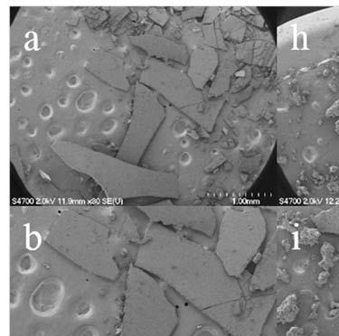
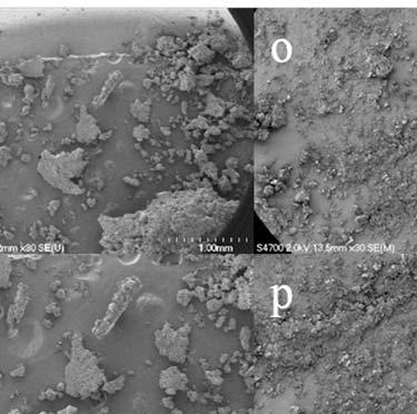
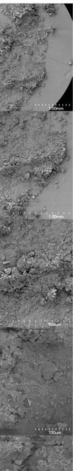
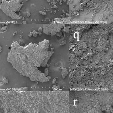
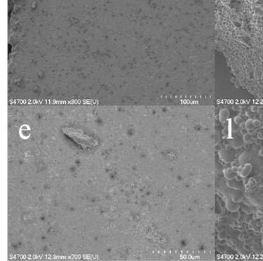
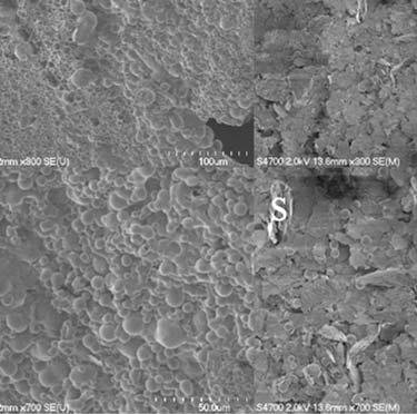
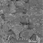
87 62

88 Figure 2.5 Surface structure of three samples with increasing magnification; Solid, Imaging from Table 2.1 is (a-g), Solid, Imaging from Table 2.1 is (h-n), Solid, Imaging from Table 2.1 is (o-u) taken at point,, and respectively are shown by SEM in magnifications of 30x (a, h, o), to 50x (b,i, p), 100x (c, j, q), 300x (d, k, r), 700x (e, l, s), 5K (f, m, t), and15kx (g, n, u). 63

89 Figure 2.6 Solid lignin and solid cellulose standards FTIR spectra 64

90 Figure 2.7 Effluent pre and post hydrolysis FTIR spectra 65

91

92 Appendix A Documentation for Fair use of Figures 2.2, 2.3 and

93 68

94 69

95

96 Chapter 3 Determination of Optimum Hydrolysis Conditions for Conversion of a Forest Product Wastewater Effluent to Fermentable Sugars 2 Jifei Liu 1, Stephanie Gleason 2, Susan T. Bagley 2, David R. Shonnard 1, 3 1 Department of Chemical Engineering 2 Department of Biological Sciences 3 The Sustainable Futures Institute Michigan Technological University, Houghton, MI Corresponding author: Jifei Liu, jifeil@mtu.edu, (906) Michigan Technological University 1400 Townsend Dr. Chemical Sciences Building Rm. 308 Houghton, MI To be submitted to Bioresource Technology 71

97 Abstract A two-step hydrolysis process was employed on a hardboard wastewater stream for determining the viability for production of mixed sugars. Five- and six- carbon sugar and inhibitor concentrations were analyzed after dilute acid hydrolysis with different acid concentrations and times of hydrolysis at 121 C. Quadratic regression models and Response Surface Method (RSM) were employed to identify optimum reaction conditions to give high sugar yields and acceptably low inhibitors levels which would not negatively influence subsequent fermentation. The optimum conditions for dilute acid pretreatment were determined to be in the range of acid concentration of %, and reaction time of minutes. It was also discovered that enzyme hydrolysis after optimum pretreatment did not produce significant amounts of sugars, thus acid pretreatment alone is sufficient. This study concludes that a hardboard wastewater stream is a promising feedstock for production of mixed sugars which may be fermented to high value products. Highlights Hardboard wastewater stream is proved a promising feedstock for production of mixed sugars. The optimum condition of acid pretreatment was determined numerically by RSM for the highest sugar yield as acid concentration in the range of % and reaction time of minutes. 72

98 Enzymatic hydrolysis (EH) is not necessary for this wastewater stream after optimum dilute acid pretreatment, yet EH is not sufficient without dilute acid pretreatment. Keywords Hardboard wastewater; dilute acid pretreatment; enzymatic hydrolysis; regression models; response surface methodology 1. Introduction Biomass resources as feedstock for the production of bioenergy have been widely accepted as a solution to fill in the gap between the growing energy requirement and reducing fossil fuel resources (Naik et al., 2010; Perlack & Stokes, 2011; Sims et al., 2010). Lignocellulosic biomass feedstock is considered a promising alternative resource to produce fuels and chemicals as it avoids competition with food (Naik et al., 2010; Sims et al., 2010). Apart from energy crops such as switchgrass and hybrid poplar, agriculture and forest biomass and industry waste resources are also of high potential (Perlack & Stokes, 2011). Novel feedstocks unused previously like forest hardboard processing wastewater is included in this scope to make full use of available biomass resources. Three main wood components; cellulose, hemicellulose and lignin, have been studied for their potential to be converted to biofuels and bioenergy. Lignin is a phenolic biopolymer that impedes enzymatic hydrolysis of cellulose and hemicellulose-degrading enzymes (Kumar et al., 2009). Cellulose and hemicellulose are polysaccharides hydrolysable by both chemical and biochemical approaches. Cellulose is a crystalline polymer consisting 73

99 of only glucoses while hemicellulose is a branched polymer consisting of various monosaccharide units such as glucose, xylose, galactose, arabinose and mannose. In addition, hemicellulose is more accessible to hydrolysis compared to cellulose due to its amorphous structure (Chandra et al., 2007; Kumar et al., 2009; Mosier et al., 2005). Thermochemical conversion and biochemical conversion are technologies applied in the biofuel production. Thermochemical conversion is usually conducted under high temperature ( C), for example pyrolysis and gasification are thermochemical processes widely studied for biomass conversion (Lange, 2007; Shonnard et al., 2012). Biochemical conversion technology employs much more gentle conditions compared to thermochemical conversion. Pretreatment and enzymatic hydrolysis are included in biochemical conversions to break down the structure of cellulose and hemicellulose into fermentable sugars (Shonnard et al., 2012). Effective pretreatments should not only solubilize or partially solubilize the structure of hemicellulose chains but also reduce the crystallinity of cellulose and make cellulose and hemicellulose more accessible to enzymes. Among the pretreatment methods studied most include dilute acid pretreatment, hydrothermal pretreatment, alkaline pretreatment, ammonia fiber expansion, and ionic fluids (Carvalheiro et al., 2008; Kumar et al., 2009; Mosier et al., 2005; Pienkos & Zhang, 2009; Shonnard et al., 2012). Dilute acid pretreatment is one of the most widely used pretreatment approaches (Kumar et al., 2009). However, during the process of acid pretreatment, some compounds inhibitory to fermentation of sugars are generated, including dehydration products from sugars, (furfural and hydroxymethylfurfural (HMF)), phenolic compounds and organic acids. These compounds may have inhibitory effects on fermentation depending on the concentration (Palmqvist & Hahn-Hägerdal, 2000; 74

100 Taherzadeh & Karimi, 2007). Therefore, the optimum acid pretreatment condition for a certain feedstock is one that maximizes the yield of fermentable sugars, as well as minimizes the level of potential inhibitors. Regression methods and response surface methodology (RSM) have been applied in analyzing data from various kinds of experiments (Montgomery, 2009), and the acid pretreatment process has been modeled to determine the optimum parameters conditions for best sugar yield and minimum inhibitors (Jeong et al., 2010; Jeya et al., 2009; Sasikumar & Viruthagiri, 2008; Rodrigues, 2012; Kim et al, 2011). Acid pretreatment is applied to increase the accessibility of cellulose to enzyme, and a subsequent enzymatic hydrolysis is usually used to further break down the structure of cellulose in the biomass materials. Therefore, the concentration of sugars after enzymatic hydrolysis account for the results of both acid pretreatment and enzymatic hydrolysis. One objective of this research was to evaluate the process of dilute acid pretreatment of a novel biofuel feedstock, a hardboard process wastewater stream, and determine the effects of acid concentration and reaction time on the yield of sugar as well as inhibitors produced. Another objective of the research was to evaluate the hydrolysis results after both acid pretreatment and enzymatic hydrolysis and to compare the results with acid pretreatment results alone, in order to understand the effect of enzyme as well as its loading (concentration). 75

101 2. Materials and method 2.1. Composition of the effluent waste materials The biofuel feedstock for this research is a wastewater stream from a wood panel manufacturing facility with 7.5% of dry solids, as determined following National Renewable Energy Laboratory (NREL) s Laboratory Analytical Procedure (LAP): Determination of structural carbohydrates and lignin in biomass. (Sluiter et al., 2008a). Most of the cellulose in the chipped hardwood was retained in the extraction process, and thus hemicellulose was hypothesized to be the main component in the wastewater to produce fermentable sugars. As determined in a prior study (see Chapter 2 for detail), the composition of the effluent solid material on a dry basis is 5% of ash, 23.5% lignin, 8.9% glucans, 34.7% xylans, 5.5% galactans, and 10.4% arabinans and mannans as determined based on NREL s Laboratory Analytical Procedure: Determination of structural carbohydrates and lignin in biomass (Sluiter et al., 2008b) Acid pretreatment and enzymatic hydrolysis condition Acid pretreatment was performed in a sealed 500ml VWR glass bottle in an autoclave at 121 C. Reaction time with six time levels (1, 30, 45, 60, 75 and 90 min) and H 2 SO 4 concentration with three levels (0%, 1%, and 2%) are two parameters considered in acid pretreatment. The 18 conditions were all carried out in duplicate starting by adding 85ml of feedstock with corresponding amount of 96% H 2 SO 4 to reach the required acid concentration. 76

102 Out of all the samples, only 30, 60, and 90 minute trials were chosen for the subsequential enzymatic hydrolysis as shown in Table 3.1. It began by collecting 50 ml of the acid hydrolysate from each pretreated sample. This 50 ml was then divided into two 25 ml samples in separate Erlenmeyer flasks (50ml). Each 25 ml sample was then neutralized to a ph of 4.6-5, which is the ph required by the enzymes. Then 1.25 ml of a 1M sodium citrate buffer (ph 4.5), was added to each sample to help maintain a ph in the sample of ~4.8. Once the buff consumption of sugars (Selig et al.,2008). The flasks were then placed into an orbital shaker (Lab-Line Orbit Environ-Shaker, Lab Line Instruments Inc., IL) at 50 C for one hour to ensure the temperature of each sample had reached 50 C. After this one hour equilibrium period, the samples were ready for the addition of enzyme. The enzymes used were, Accellerase 1500 (DuPont Industrial Biosciences), and Accellerase XY (DuPont Industrial Biosciences). Accellerase 1500 contains exoglucanase, endoglucanase, hemi-cellulase, betaglucosidase and others, which are effective for cellulose, hemicellulose and -glucans. Accellerase XY contains xylanse, and usually is used to supplement cellulase. Two dosage levels, low and high were chosen as shown in Table 3.2. Once the enzymes were added, the samples were placed back in the orbital shaker for 72 hours at 50 o C. 1-mL samples were collected at 24, 48, and 72 hours and filtered through a before analyzed for the concentrations of monomer sugars and degradation products. 77

103 2.3. Concentration analysis Acid pretreatment results and enzymatic hydrolysis results were analyzed by high performance liquid chromatography (Agilent 1200 Series HPLC) with a Bio-Rad Aminex HPX-87P column. Monomer sugars (glucose, xylose, galactose, arabinose and mannose) released from the two processes were detected by a refractive index detector, whereas the inhibitors generated (furfural and (HMF)) were analyzed by a diode-array detector (DAD)(see section 3.2 of Chapter 2 for details) 2.4. Statistical analysis RSM were performed by the software Design-Expert 8.0 (Stat Ease, Inc., Minneapolis, USA) to evaluate the combined effect of parameters on the responses and to estimate the optimum condition for acid pretreatment and enzymatic hydrolysis. A quadratic model was expressed in equation (1) to predict the relation between responses (dependent variables) (y, monomer sugar yields (Y Monomer Sugars ), total sugar yield (Y Total Sugar ), inhibitor yields (Y Inhibitors ), and the variables (reaction time and acid concentration)), + (1) where y refers to the response variables, x 1 and x 2 represent reaction time and acid concentration, respectively, i are the coefficients to be determined, and are random errors. The yields of sugars or inhibitors are expressed as Y Sugars or Y Inhibitors and defined 78

104 as the concentration of sugars or of inhibitors divided by the concentration of total solid in the feedstock (77.03g/l as shown in Chapter 2). Hydrolysis results post enzymatic hydrolysis were modeled as equation (2), where y represents sugar yield (monomer sugars and total sugar yield) after enzymatic hydrolysis. x 3 is the enzyme loading of Accellerase y= + x + x + x + x + x + x + x x + x x + x x (2) The significance of each quadratic term (any term involving x i multiplied by x i ) was evaluated. Quadratic terms with P-values over 0.05 were considered insignificant and removed from the model. The relations between the response variable y and the variables of both equations (1) and (2) were then tested through P-value, which is the probability that statistic will take on a value that is at least as extreme as the observed value of the statistic when the null hypothesis H 0 is true (Montgomery, 2009), as well as R 2, which is defined as the sum of squares corresponding to the model divided by the total sum of squares. The adjusted R 2 is more useful in complex experiments with several factors as it reflects the numbers of factors in the model; thus it is also referred to in the research. The models were also compared to the experimental data when one factor is fixed. The variable values leading to the optimum responses were determined by numerical analysis with Design-Expert

105 3. Results and discussion 3.1. Sugar and inhibitory compounds generated during acid pretreatment The key result from this hydrolysis study is that total monomer sugar concentrations increase with increasing acid concentration for any fixed reaction time and also increase with increasing reaction time for any fixed acid concentration, as shown in Figure 3.1. The exceptions to this trend are when the autoclave time reaches 90 minutes, the monomer sugar concentrations begin to decrease for acid levels of 1% and 2% due to conversion of monomer sugars to dehydration products. This suggests that the optimum condition of acid pretreatment is within the range of our matrix. The baseline shows total monomer sugar concentration before acid pretreatment. More results of monomer and total sugars are shown in section 1.1 of Appendix B. Hydroxymethyl furfural and furfural concentrations of samples undergoing different experiment conditions are displayed in Figure 3.2. As discussed in Chapter 1, most of the previous studies show that when the concentration of furfural is below 0.5 g/l, the inhibition is not strong enough to be observed on Scheffersomyces stipitis (Mussatto & Roberto, 2004). HMF is expected to exhibit a less toxic effect due to lower formation rate and lower concentration than furfural. Results presented here indicate that the higher the acid concentration and the longer the experiment time, the more HMF and furfural were generated. That means that when more monomer sugars are generated at high acid concentration and long time, more HMF and furfural are produced. Thus, the object was to reach a balance. More HMF and furfural 80

106 results can be found in section 1.2 of Appendix B. HMF and Furfural results compared with concentrations of monomer sugars are displayed in section 1.3 of Appendix B Sugar yield after enzymatic hydrolysis Total monomer sugar yield after 72 hours of enzymatic hydrolysis are compared with acid pretreatment only (AP) results in Figure 3.3. These data generally show that the higher loading of enzyme results in more monomer sugar production. This trend is especially true for 0% and 1% dilute acid pretreatment. However, for the samples that already exceeded 30 g/l produced after dilute acid hydrolysis, few additional monomer sugars were released during subsequent enzymatic hydrolysis, and less difference due to the enzyme loading was observed compared to dilute acid hydrolysis only Statistical Analysis The experimental data from 18 trials used to build up the regression models are displayed in Table 3.3a and Table 3.3b, including seven response variables as well as two variables reaction. From the seven responses modeled to understand the effect of acid pretreatment, monomer sugars (glucose, xylose, galactose, arabinose and mannose) yields and total sugars yield were fitted in quadratic regression models as shown in equation (3)-(7) with two variables reaction time ( ) and acid concentrations ( ). These five models are all significant with the P-values less than , and R 2 over 0.90, explaining more than 90% of the variability in responses. The adjusted R 2 are in reasonable agreement with R 2. (3) 81

107 (4) (5) (6) (7) Response surfaces were generated using the equation for total monomer sugar (eqn. 7) and are shown in Figure 3.4. Table 3.4 is a summary of the results of all responses in their highest values together with the correspongding values of the variables as well as R 2, adj R 2, and P-value. The optimum total sugar yield was found when autoclave time is 90 minutes and acid concentration is 1.97%. Similarly, the maximum yield of glucose, xylose and galactose are all found in autoclave time range ( ), and acid concentration (1.73%-2.00%). The maximum yield of arabinose and mannose, on the other hand, were found when autoclave time is 1 minute, indicating that arabinose and mannose require much shorter time to be released, and the reaction is more sensitive to acid concentration than autoclave time. However, arabinose and mannose make up only a small portion of total sugars, so this result does not have significant influence on total sugar production. Response surface of monomer sugars glucose, xylose, galactose, arabinose and monnose are displayed in Figure B.29-B.32 in section 3.1 of Appendix B. In order to understand the regression model better, predicted total sugar yields in certain circumstances (constant reaction times or acid concentrations) are compared with the actual total sugar yields in Figure 3.5. The regression model shown in Figure 3.5a shows 82

108 that for a given acid concentrations, total sugar yields increase linearly with the reaction time. The regression model correctly shows higher yields with higher acid concentration. However, the data show a more complicated trend with increasing reaction time. The data exhibits a delayed then increasing yield trend at early times, a more linear increase at intermediate times, and then a slight decrease at long times, for the 1 and 2% acid concentration data. The regression model realistically predicts yield increase with reaction time and acid concentration, but is not able to account for the non-linear behavior in the data. In Figure 3.5b, total sugar yield is plotted versus increasing acid concentration for each reaction time. The regression model exhibits a non-linear concave downward trend with increasing acid concentration with a maxium near 2% acid. But some of the data in Figure 3.5b show a different response. For 90 minutes reaction time, yield declines between 1 2% acid concentration due to dehydration reactions of monomer sugars to produce furfural and HMF. HMF and furfural were modeled in equation (8) and (9). In these two models, only the x 1 x 2 term in equation (9) is significant out of all quadratic terms. The range of these responses are shown in Table 3.4. As shown in Figure 3.6 and 3.7, yield of furfural is approximately less than 0.01 and for HMF yield it is less than for all reaction conditions, indicating that the concentrations of furfural and HMF are less than 0.78 g/l and 0.11g/l, respectively, in the range of experimental conditions. Figure 3.6a shows a linear increase in predicted HMF yield with increasing reaction time for all acid levels, and the model fit is most favorable for the 1% acid data. In Figure 3.6b, the data shows an increase in HMF yield with increasing acid% with the exception for the 75 minute data, consistent with the model predictions. The regression model for furfural is compared to data in Figures 3.7a and b, 83

109 with good fit between data and the model. The data and model exhibits increasing yield of furfural with increasing time for constant acid level and with increasing acid level for constant time. The linear trends in furfural yield predicted by the model are in contrast with the total monomer sugar and HMF model predictions in that the slopes of the model lines for furfural increase with increase in acid level and reaction time for Figures 3.7a and b, respectively. The maximum concentration of furfural is 0.78g/l while that of HMF is 0.11g/l. HMF and furfural in these concentrations may have some inhibitory effect on the subsequent fermentation step using S. stipitis CBS 6054 (Groves et al., 2013). According to previous studies on inhibitory effect of HMF and furfural, the optimum conditions of acid pretreatment should be determined while the concentration of furfural is less than 0.5 g/l to avoid the inhibition (Mussatto & Roberto, 2004). Therefore, the optimum conditions of acid pretreatment should exclude those resulting in furfural concentrations more than 0.5 g/l. The yellow line in Figure 3.8 represents 0.5 g/l of furfural concentration (see Figure B 34 in Appendix B for detail). This yellow line and the contour representing 0.58 of total sugar yield together form a green area, which is the optimum conditions resulting in total sugar concentrations over 44.8 g/l and furfural concentrations less than 0.5 g/l. Y = x x (8) Y = x x x x (9) 84

110 In enzymatic hydrolysis experiments conducted after neutralizing dilute acid hydrolysate, inhibitor levels remained the same, but additional amount of sugar was released. Therefore, the effect of three variables (acid pretreatment time, acid concentration, and enzyme loading) in the two stages (dilute acid hydrolysis followed by enzymatic hydrolysis) were evaluated together. All dependent variables and variables in various hydrolysis conditions are shown in Table 3.5. The yield of total sugar as well as glucose, xylose, galactose, and arabinose and mannose were fit to regression models with the three variables in equation (10)-(14). All model fits are significant (P<0.0001), and the significance of the models were also verified by the coefficients of determination as shown in Table 3.6 (R 2 >0.9000). Table 3.6 also displayes the maximum value of each response calculated from the models as well as the reaction condition for this maximum. It can be summerized that the highest yield of glucose and galactose does not require much enzyme, which might be because the glucans and galactans are mostly hydrolyzed into glucoses and glactoses during acid pretreatment. The highest yield of arabinose and mannose show up in short autoclave times, meaning arabinose and mannose could be released into the liquid shortly after acid pretreatment starts. Xylose, on the other hand, requires much longer reaction time and more enzyme loading. As the amount of xylose is the most among the five monomor sugars, the optimum condition for total sugars is most influenced by the optimum condition for xylose. A three dimentional cubic model showing total sugar yield after the two stage hydrolysis is displayed in Figure 3.9, each direction representing one variable, thus each point in the cubic model locks a certain hydrolysis condition. Through numerical calculation from the model, the maximum total sugar yield of was shown in the figure as the optimum 85

111 solution out of all points representing all solutions distributed in the cube with various reaction conditions. It can be observed from Figure 3.9 that when acid concentration is high enough, enzyme loading and autoclave time both have limited influence to the total sugar yield. Similar results can be observed from cubic models of individual monomer sugars shown as Figure B.37-B.40 in section 3.3 of Appendix B. As discussed in section 2.2, experimental data of three acid pretreatment time, two acid concentration and two enzyme loading levels resulted in a list of numerical solutions for the two stage hydrolysis as shown in Table 3.7. The total sugar yields in the first ten solutions (the fourth column) have little differences, unlike reaction time (the first column), which are all in the range of 85 ~ 90 minutes; or acid concentration (the second column), which are all in the range of 1.2~2.0 %, enzyme loading varies from 0.05 to This proves that multiple combinations of the three varibles could result in very similar results, the loss of total sugar yield from the decrease of one variable can be made up by increasing another one. The optimun total sugar yields require acid concentration and reaction time in a certain range, but the effect of enzyme loading on total sugar yields is very little. Taken together, results from this study show that in the hydrolysis of hardboard wastewater stream, enzyme is not necessary as it does not contribute significant amount of additional sugars after an efficient acid pretreatment. y = x x x x x x (10) 86

112 y = x x x x x x (11) y = x x x x x x x x x (12) y = x x x x x (13) y = x x x x x x (14) Several studies have attempted to find the optimum conditions of acid pretreatment using the RSM for various feedstocks such as barley straw and rapeseed straw (Kim et al., 2011; Jeong et al., 2010). Typical conditions analyzed with RSM in these studies include reaction time, temperature, and acid concentration. However, in these studies optimum conditions identified by RMS method did not consider inhibitory effects from the byproducts generated from acid pretreatment, as my study did. In addition, previous studies determined the optimum conditions of enzymatic hydrolysis for various feedstocks such as maize starch, sapodilla juice and wheat straw with RSM (Kunamneni and Singh, 2005; Sin et al., 2005; Qi, 2009). Enzyme dose, incubation time and ph are typical factors studied, and the optimum conditions determined vary depending on the feedstocks and the pretreatment methods. The RMS has been employed often in the literature to aid in identification of optimum conversion conditions, however it is difficult 87

113 to make direct comparisons between the various studies due to differences in feedstocks and pretreatment processes. The models set up in this statistical analysis, however, have some limitations in precisely describing the trend of the experimental data. First of all, there are only 18 runs analyzed in the regression surface methodology, therefore more experimental data and more repeated runs would help improve model fit to the data and reduce uncertainties. Furthermore, usually low order models (first or second order) are applied (Montgomery, 2009), however, second order models may not be accurate to describe the kinetic relation between dependent variables and the variables, and higher order models may be needed to describe the trend of the experimental data better. Apart from that, the optimum conditions chosen by this method include multiply combinations of reaction time and acid concentration. In order to apply the results in this study to commercial production of ethanol, a thorough economic analysis would be necessary to understand the effects of reaction conditions on process economics. 4. Conclusion Hardboard wastewater is a potential feedstock for the production of ethanol as a xylansrich biomass material. Monomer sugars generated during dilute acid pretreatment alone is a good start for generating mixed sugars for possible high-value product formation through fermentation with inhibitor concentrations below threshold values. The optimum conditions for dilute acid pretreatment were determined to be in the range of acid concentration ( %), and reaction time (48-76 minutes) by RSM, however further study refinements require an economic analysis. We also conclude that enzyme is 88

114 not necessary for the high sugar yield with this type of material as hardboard processing wastewater. 5. Acknowledgements We acknowledge the financial support of the Michigan Economic Development Corporation (MEDC) by grant No. DOC-1751 through the Center of Energy Excellence program. 89

115 Tables Table 3.1. Experimental matrix regarding acid pretreatment and enzymatic hydrolysis proceeded (The temperature of the experiments were all conducted at 121 o C) Reaction Time (min) 60min 90min 1min 45min 75min 30min. 0% AP&EH AP&EH AP&EH AP AP AP 1% AP&EH AP&EH AP&EH AP AP AP 2% AP&EH AP&EH AP&EH AP AP AP Acid Percentage (%) a AP Acid Pretreatment; b EH-Enzymatic Hydrolysis 90

116 Table 3.2. High and low enzyme dosage in enzymatic hydrolysis Accellerase 1500 Accellerase XY High Dosage 0.5ml(0.25 ml/gram of biomass) 0.1ml(0.05ml/gram of biomass) Low Dosage 0.1 ml(0.05ml/gram of biomass) 0.01ml(0.005ml/gram of biomass) 91

117 Table 3.3a. Responses Obtained under different acid pretreatment conditions. The unit of yield is expressed as. Run Autoclave Time (min) Variables Responses y (dependent variables) Acid Concentration (%) Y Glucose YXylose YGalactose YArabinose +Mannose YTotal Sugar

118 Table 3.3b. Responses Obtained under different acid pretreatment conditions, the unit of yield is expressed as. Variables Responses y (dependent variables) Acid Concentration (%) Y HMF YFurfural Autoclave Time (min) Run

119 Table 3.4. Optimum condition and ANOVA analysis results after acid pretreatment. The unit of yield is expressed as. Responses y Predicted Value Optimum Condition ANOVA Autoclave Time (min) Acid Concentration (%) R2 Adj R 2 P-value YGlucose < YXylose < YGalactose < YArabinose + Mannose < YTotal sugar <

120 Table 3.5. Regression model responses obtained under different hydrolysis conditions. The unit of yield is expressed as. Run Autoclave Time Acid Concentration (%) Variables Responses y (dependent variables) Enzyme Loading (ml/gram of dry biomass) YGlucose YXylose YGalactose YArabinose +Mannose YTotal Sugar 95

121 Table 3.6. Optimum condition and ANOVA analysis results after hydrolysis. The unit of yield is expressed as. Responses y Predicted Value Optimum Condition ANOVA Autoclave Time (min) Acid Concentration (%) Enzyme Loading (ml/gram of biomass) R2 Adj R 2 P-value YGlucose < YXylose < YGalactose < YArabinose + Mannose < YTotal sugar <

122 Table 3.7. Predicted results of enzymatic hydrolysis from the regression model for total sugar yield. The unit of yield is expressed as. Enzyme Loading (ml/gram Autoclave Time (min) Acid Concentration (%) of biomass) YTotal Sugar

123 Figures 60 1min Concentration(g/L) Acid Concentration (%) 30min 45min 60min 75min 90min Total sugar level before acid pretreatmen Figure 3.1 Comparison of the total monomer sugar concentrations after each acid pretreatment trial (The results are average of two replicates and the error bar is +/- one standard deviation). Concentration (g/l) g/l line for furfural Acid Concentration (%) Furfural 1min HMF 1min Furfural 30min HMF 30min Furfural 45min HMF 45min Furfural 60min HMF 60min Furfural 75min HMF 75min Furfural 90min HMF 90min Figure 3.2 HMF and furfural concentrations after different acid pretreatment trials (The results are average of two replicates and the error bar is +/- one standard deviation). 98

124 Concentration (g/l) Autoclave Time (min) 0% Acid High 0% AP 1% Acid High 1% AP 2% Acid High 2% AP 0% Acid Low 0% AP 1% Acid Low 1% AP 2% Acid Low 2% AP Figure 3.3 Comparison of the total monomer sugar concentrations after 72 hr of enzymatic hydrolysis (The results are average of two replicates and the error bar is +/- one standard deviation, the crossed bars in the same color represent the total monomer sugars before enzymatic hydrolysis starts under certain acid pretreatment condition. One color represents one acid pretreatment condition, high and low are loading of enzyme). AP is acid pretreatment only; with no enzymes added after AP. 99

125 Figure 3.4 Effect of A:autoclave time (min) and B: acid concentration (%) on total sugar yield (total sugar yield plotted in 3D surface (a) and contour (b) plots) 100

126 Yield a Regression Model (Acid Concentration = 0%) Regression Model (Acid Concentration = 1%) Regression Model (Acid Concentration = 2%) Experimental Data (Acid Concentration = 0%) Experimental Data (Acid Concentration = 1%) Experimental Data (Acid Concentration = 2%) Reaction Time (min) b 0.5 Yield 0.4 Experimental Data (Reaction Time = 1 min) Experimantal Data (Reaction Time = 30 min) 0.3 Experimantal Data (Reaction Time = 45 min) Experimantal Data (Reaction Time = 60 min) Experimantal Data (Reaction Time = 75 min) 0.2 Experimantal Data (Reaction Time = 90 min) Regression Model (Reaction Time = 1min) Regression Model (Reaction Time = 30 min) 0.1 Regression Model (Reaction Time = 45 min) Regression Model (Reaction Time = 60 min) Regression Model (Reaction Time = 75 min) Regression Model (Reaction Time = 90 min) Acid Concentration (%) Figure 3.5 Comparison of predicted total sugar yields from the regression models with experimental data at fixed reaction time or acid concentration. (a) Predicted total sugar yields (lines) compared with experimental data (points) at fixed acid concentrations (The results are average of two replicates and the error bar is +/- standard deviation). (b) Predicted total sugar yields (lines) compared with experimental data (points) at fixed acid concentrations. 101

127 Yield Yield 1.8E E E E E E E E E E E E E E E E E E E Reaction Time (min) Regression Model (Acid Concentration = 0%) Regression Model (Acid Concentration = 1%) Regression Model (Acid Concentration = 2%) Experimental Data (Acid Concentration = 0%) Experimental Data (Acid Concentration = 1%) Experimental Data (Acid Concentration = 2%) Acid Concentration (%) Experimental Data (Reaction Time = 1 min) Experimental Data (Reaction Time = 30 min) Experimental Data (Reaction Time = 45 min) Experimental Data (Reaction Time = 60 min) Experimental Data (Reaction Time = 75 min) Experimental Data (Reaction Time = 90min) Regression Model (Reaction Time = 1 min) Regression Model (Reaction Time = 30 min) Regression Model (Reaction Time = 45 min) Regression Model (Reaction Time = 60 min) Regression Model (Reaction Time = 75 min) Regression Model (Reaction Time = 90 min) Figure 3.6 Comparison of predicted HMF yields from the regression models with experimental data at fixed reaction time or acid concentration. (a) Predicted HMF yields (lines) compared with experimental data (points) at fixed acid concentrations. (The results are average of two replicates and the error bar is +/- one standard deviation.) (b) Predicted HMF yields (lines) compared with experimental data (points) at fixed acid concentrations. a b 102

128 Yield 1.2E E E E E E E E E E E Reaction Time (min) Regression Model (Acid Concentration = 0%) Regression Model (Acid Concentration = 1%) Regression Model (Acid Concentration = 2%) Experimental Data (Acid Concentration = 0%) Experimental Data (Acid Concentration = 1%) Experimental Data (Acid Concentration = 2%) a b Yield 6.0E E E E E Acid Concentration (%) Experimental Data (Reaction Time = 1 min) Experimental Data (Reaction Time = 30 min) Experimental Data (Reaction Time = 45 min) Experimental Data (Reaction Time = 60 min) Experimental Data (Reaction Time = 75 min) Experimental Data (Reaction Time = 90 min) Regression Model (Reaction Time = 1 min) Regression Model (Reaction Time = 30 min) Regression Model (Reaction Time = 45 min) Regression Model (Reaction Time = 60 min) Regression Model (Reaction Time = 75 min) Regression Model (Reaction Time = 90 min) Figure 3.7 Comparison of predicted furfural yields from the regression models with experimental data at fixed reaction time or acid concentration. (a) Predicted furfural yields (lines) compared with experimental data (points) at fixed acid concentrations. (The results are average of two replicates and the error bar is +/- one standard deviation.) (b) Predicted furfural yields (lines) compared with experimental data (points) at fixed acid concentrations. 103

129 Figure 3.8 Optimum conditions (A: autoclave time (min) and B: acid concentration (%)) for acid pretreatment highlighted in contour plot of total sugar yield. Reaction conditions of time and acid concentration to the right and above should be avoided in order to control furfural and HMF inhibitor levels. 104

130 Figure 3.9 Effect of A: autoclave time (min), B: acid concentration (%) and C: enzyme loading (ml/gram of dry biomass) on total sugar yield 105

131 References Carvalheiro, F., Duarte, L.C., Gírio, F.M Hemicellulose biorefineries: a review on biomass pretreatments. Journal of Scientific & Industrial Research, 67, Chandra, R.P., Bura, R., Mabee, W.E., Berlin, A., Pan, X., Saddler, J.N Substrate Pretreatment: The Key to Effective Enzymatic Hydrolysis of Lignocellulosics? in: Biofuels, (Ed.) L. Olsson, Vol. 108, Springer Berlin Heidelberg, pp Groves, S., Liu, J., Shonnard, D., Bagley, S Evaluation of hardboard manufacturing process wastewater as a feedstream for ethanol production. Journal of Industrial Microbiology & Biotechnology, 1-7. Jeong, T.-S., Um, B.-H., Kim, J.-S., Oh, K.-K Optimizing dilute-acid pretreatment of rapeseed straw for extraction of hemicellulose. Applied biochemistry and biotechnology, 161(1-8), Jeya, M., Zhang, Y.-W., Kim, I.-W., Lee, J.-K Enhanced saccharification of alkalitreated rice straw by cellulase from Trametes hirsuta and statistical optimization of hydrolysis conditions by RSM. in: Bioresource Technology, Vol. 100, pp Kim, S.B., Lee, J.H., Oh, K.K., Lee, S.J., Lee, J.Y., Kim, J.S., Kim, S.W Dilute acid pretreatment of barley straw and its saccharification and fermentation. Biotechnology and Bioprocess Engineering, 16(4), Kumar, P., Barrett, D.M., Delwiche, M.J., Stroeve, P Methods for Pretreatment of Lignocellulosic Biomass for Efficient Hydrolysis and Biofuel Production. Industrial & Engineering Chemistry Research, 48(8), Kunamneni, A., Singh, S Response surface optimization of enzymatic hydrolysis of maize starch for higher glucose production. Biochemical Engineering Journal, 27(2), Lange, J.P Lignocellulose conversion: an introduction to chemistry, process and economics. Biofuels, Bioproducts and Biorefining, 1(1), Montgomery, D.C Design and analysis of experiments. seventh ed. John Wiley & Son, Inc. Mosier, N., Wyman, C., Dale, B., Elander, R., Lee, Y.Y., Holtzapple, M., Ladisch, M Features of promising technologies for pretreatment of lignocellulosic biomass. Bioresource Technology, 96(6), Mussatto, S.I., Roberto, I.C Alternatives for detoxification of diluted-acid lignocellulosic hydrolyzates for use in fermentative processes: a review. Bioresource Technology, 93(1), Naik, S.N., Goud, V.V., Rout, P.K., Dalai, A.K Production of first and second generation biofuels: A comprehensive review. Renewable & Sustainable Energy Reviews, 14(2), Palmqvist, E., Hahn-Hägerdal, B Fermentation of lignocellulosic hydrolysates. II: inhibitors and mechanisms of inhibition. Bioresource Technology, 74(1), Perlack, R.D., Stokes, B.J US billion-ton update: biomass supply for a bioenergy and bioproducts industry. Oak Ridge National Laboratory. ORNL/TM-2011/224. Pienkos, P., Zhang, M Role of pretreatment and conditioning processes on toxicity of lignocellulosic biomass hydrolysates. Cellulose, 16(4),

132 Qi, B., Chen, X., Shen, F., Su, Y., Wan, Y Optimization of enzymatic hydrolysis of wheat straw pretreated by alkaline peroxide using response surface methodology. Industrial & Engineering Chemistry Research, 48(15), Rodrigues, R.C., Kenealy, W.R., Dietrich, D., Jeffries, T. W Response surface methodology (RSM) to evaluate moisture effects on corn stover in recovering xylose by DEO hydrolysis. Bioresource technology, 108, Sasikumar, E., Viruthagiri, T Optimization of process conditions using response surface methodology (RSM) for ethanol production from pretreated sugarcane bagasse: kinetics and modeling. BioEnergy Research, 1(3-4), Selig, M.J., Viamajala, S., Decker, S.R., Tucker, M.P., Himmel, M.E., Vinzant, T.B Deposition of lignin droplets produced during dilute acid pretreatment of maize stems retards enzymatic hydrolysis of cellulose. Biotechnology Progress, 23(6), Shonnard, D.R., Campbell, M.B.-., Martin-Garcia, A.R., Kalnes, T.K Chemical Engineering of Bioenergy Plants: Concepts and Strategies. in: Handbook of bioenergy crop plants, (Eds.) C. Kole, C.P. Joshi, D.R. Shonnard, pp Sims, R.E.H., Mabee, W., Saddler, J.N., Taylor, M An overview of second generation biofuel technologies. Bioresource Technology, 101(6), Sin, H.N., Yusof, S., Sheikh Abdul Hamid, N., Rahman, R.A Optimization of enzymatic clarification of sapodilla juice using response surface methodology. Journal of Food Engineering, 73(4), Sluiter, A., Hames, B., Hyman, D., Payne, C., Ruiz, R., Scarlata, C., Sluiter, J., Templeton, D., Wolfe, J. 2008a. Determination of Total Solids in Biomass and Total Dissolved Solids in Liquid Process Samples Laboratory Analytical Procedure Cole Boulevard, Golden, Colorado. Sluiter, A., Hames, B., Ruiz, R., Scarlata, C., Sluiter, J., Templeton, D., Crocker, D. 2008b. Determination of structural carbohydrates and lignin in biomass, National Renewable Energy Laboratory Cole Boulevard, Golden, Colorado Selig M., Weiss N., Ji Y Enzymatic saccharification of lignocellulosic biomass, National Renewable Energy Laboratory Cole Boulevard, Golden, Colorado Taherzadeh, M.J., Karimi, K Acid-based hydrolysis processes for ethanol from lignocellulosic materials: A review. Bioresources, 2,

133

134 Appendix B 1. Acid Pretreatment (AP) Results 1.1. Monomer and Total Sugar Figures B.1-B.6 show the individual monomer sugar, total monomer sugar, and cellobiose present after different AP trials. These figures include a line at the total monomer sugar concentration prior to any treatment of the API effluent. Concentration (g/l) Total Sugar Glucose Xylose Galactose Arabinose and Mannose Cellobiose Acid Percentage Total sugar level before acid pretreatment Figure B.1 Total and individual monomer sugar concentrations after 1min AP (The results are average of two replicates and the error bar is +/- one standard deviation.) 109

135 60 50 Total Sugar Xylose Arabinose and Mannose Glucose Galactose Cellobiose Concentration (g/l) Acid Percentage Total sugar level before acid pretreatment Figure B.2 Total and individual monomer sugar concentrations after 30min AP (The results are average of two replicates and the error bar is +/- one standard deviation.) Total Sugar Xylose Arabinose and Mannose Glucose Galactose Cellobiose 40 Concentration (g/l) Total sugar level before acid pretreatment Acid Percentage Figure B.3 Total and individual monomer sugar concentrations after 45min AP (The results are average of two replicates and the error bar is +/- one standard deviation.) 110

136 60 50 Total Sugar Xylose Arabinose and Mannose Glucose Galactose Cellobiose Concentration (g/l) Acid Percentage Total sugar level before acid pretreatment Figure B.4 Total and individual monomer sugar concentrations after 60min AP (The results are average of two replicates and the error bar is +/- one standard deviation.) Total Sugar Xylose Arabinose and Mannose Glucose Galactose Cellobiose Concentration (g/l) Acid Percentage Total sugar level before acid pretreatment Figure B.5 Total and individual monomer sugar concentrations after 75min AP (The results are average of two replicates and the error bar is +/- one standard deviation.) 111

137 60 50 Total Sugar Glucose Xylose Galactose Arabinose and Mannose Cellobiose Concentration (g/l) Acid Percentage Total sugar level before acid pretreatment Figure B.6 Total and individual monomer sugar concentrations after 90min AP (The results are average of two replicates and the error bar is +/- one standard deviation.) Figures B.7-B.12 display the individual monomer sugars present after AP stacked upon each other. This shows each monomers individual contribution to the total sugar concentration. This representation makes it very easy to see the individual contributions toward total monomer sugar concentration, but difficult to compare the trends between the individual monomer sugars. 112

138 Concentration (g/l) Acid Percentage Arabinose and Mannose Galactose Xylose Glucose Figure B.7 Total and individual monomer sugar concentrations stacked after 1 min AP (The results are average of two replicates and the error bar is +/- one standard deviation.) 113

139 60 50 Arabinose and Mannose Concentration (g/l) Acid Percentage Galactose Xylose Glucose Figure B.8 Total and individual monomer sugar concentrations stacked after 30 min AP (The results are average of two replicates and the error bar is +/- one standard deviation.) Concentration (g/l) Acid Percentage Arabinose and Mannose Galactose Xylose Glucose Figure B.9 Total and individual monomer sugar concentrations stacked after 45 min AP (The results are average of two replicates and the error bar is +/- one standard deviation.) 114

140 Concentration (g/l) Acid Percentage Arabinose and Mannose Galactose Xylose Glucose Figure B.10 Total and individual monomer sugar concentrations stacked after 60 min AP (The results are average of two replicates and the error bar is +/- one standard deviation.) Concentration (g/l) Acid Percentage Arabinose and Mannose Galactose Xylose Glucose Figure B.11 Total and individual monomer sugar concentrations stacked after 75 min AP (The results are average of two replicates and the error bar is +/- one standard deviation.) 115

141 Concentration (g/l) Acid Percentage Arabinose and Mannose Galactose Xylose Glucose Figure B.12 Total and individual monomer sugar concentrations stacked after 90 min AP (The results are average of two replicates and the error bar is +/- one standard deviation.) 1.2.Hydroxymthyl furfural (HMF) and furfural Hydroxymethyl Furfural and Furfural Analysis after Acid Pretreatment Hydroxymethyl furfural and furfural concentrations of samples undergone different experiment conditions are displayed in Figure B.13, the higher the acid concentration, the longer the experiment time, the more HMF and furfural were generated. That means, when more monomer sugars were generated, more HMF and Furfural were collected too. 116

142 Concentration (g/l) Acid Percentage Furfural 1min HMF 1min Furfural 30min HMF 30min Furfural 45min HMF 45min Furfural 60min HMF 60min Furfural 75min HMF 75min Furfural 90min HMF 90min Figure B.13 HMF and furfural concentrations after different AP trials. (The results are average of two replicates and the error bar is +/- one standard deviation.) Figures B.14-B.19 show the Furfural and HMF concentrations after each AP trial Concentration (g/l) HMF Furfural Acid Percentage Figure B.14 Furfural and HMF concentrations after 1 min (The results are average of two replicates and the error bar is +/- one standard deviation.) 117

143 Concentration (g/l) HMF Furfural Acid Percentage Figure B.15 Furfural and HMF concentrations after 30 min AP (The results are average of two replicates and the error bar is +/- one standard deviation.) Concentration (g/l) HMF Furfural Acid Percentage Figure B.16 Furfural and HMF concentrations after 45 min AP (The results are average of two replicates and the error bar is +/- one standard deviation.) 118

144 Concentration (g/l) HMF Furfural Acid Percentage Figure B.17 Furfural and HMF concentrations after 60 min AP (The results are average of two replicates and the error bar is +/- one standard deviation.) 0.60 Concentration (g/l) HMF Furfural Acid Percentage Figure B.18 Furfural and HMF concentrations after 75 min AP 119

145 Concentration (g/l) HMF Furfural Acid Percentage Figure B.19 Furfural and HMF concentrations after 90 min AP (The results are average of two replicates and the error bar is +/- one standard deviation.) Figures B.20-B.25 show the monomer sugars present after each AP trial along with HMF and furfural (the fermentation inhibitors). These graphs help show the relationship between monomer sugar generation and fermentation inhibitor generation during the AP trials. 120

146 Concentration (g/l) Total Sugar Glucose Xylose HMF Furfural Acid Percentage 0.00 Figure B.20 Monomer sugar, HMF, and Furfural concentrations following a 1 min AP (The results are average of two replicates and the error bar is +/- one standard deviation.) 121

147 Concentration (g/l) Total Sugar Glucose Xylose HMF Furfural Acid Percentage Figure B.21 Monomer sugar, HMF, and Furfural concentrations following a 30 min AP (The results are average of two replicates and the error bar is +/- one standard deviation.) Concentration (g/l) Total Sugar Glucose Xylose HMF Furfural 0 1 Acid Percentage Figure B.22 Monomer sugar, HMF, and Furfural concentrations following a 45 min AP (The results are average of two replicates and the error bar is +/- one standard deviation.) 122

148 Concentration (g/l) Total Sugar Glucose Xylose HMF Furfural Acid Percentage Figure B.23 Monomer sugar, HMF, and Furfural concentrations following a 60 min AP (The results are average of two replicates and the error bar is +/- one standard deviation.) Concentration (g/l) Total Sugar Glucose Xylose HMF Furfural Acid Percentage Figure B.24 Monomer sugar, HMF, and Furfural concentrations following a 75 min AP (The results are average of two replicates and the error bar is +/- one standard deviation.) 123

149 Concentration (g/l) Total Sugar Glucose Xylose HMF Furfural Acid Percentage 0.00 Figure B.25 Monomer sugar, HMF, and Furfural concentrations following a 90min AP (The results are average of two replicates and the error bar is +/- one standard deviation.) 2. Enzymatic Hydrolysis (EH) Results Figures B.26-B28 show the contribution of the enzyme toward total sugar concentrations throughout the EH trials. The enzymes used were, Accellerase 1500 (Genencor) and Accellerase XY (Genencor) with two dosage level, low and high. The amounts used for the high and low loadings are given in Table

150 % Acid High 1% Acid High 2% Acid High 0% Acid Low 1% Acid Low 2% Acid Low Concentration (g/l) EH Time (hr) Figure B.26 Total monomer sugar concentrations throughout the EH after 30 min AP (The results are average of two replicates and the error bar is +/- one standard deviation.) Concentration (g/l) % Acid High 1% Acid High 2% Acid High 0% Acid Low 1% Acid Low 2% Acid Low EH Time (hr) Figure B.27 Total monomer sugar concentrations throughout the EH after 60 min AP (The results are average of two replicates and the error bar is +/- one standard deviation.) 125

151 % Acid High 1% Acid High 2% Acid High 0% Acid Low 1% Acid Low 2% Acid Low Concentration (g/l) EH Time (hr) Figure B.28 Total monomer sugar concentrations throughout the EH after 90 min AP (The results are average of two replicates and the error bar is +/- one standard deviation.) 3. Statistical Analysis Results 3.1. Optimum Conditions of Each Individual Sugar Figures B.29-B.32 show the response surface results of each monomer sugars (arabinose and mannose were analyzed together). The predicted optimum value was shown in the flags. 126

152 Figure B.29 Effect of A: autoclave time and B: acid concentration on glucose yield (3D surface (a) and contour (b)) 127

153 Figure B.30 Effect of A: autoclave time and B: acid concentration on xylose yield (3D surface (a) and contour (b)) 128

154 Figure B.31 Effect of A: autoclave time and B: acid concentration on Galactose yield (3D surface (a) and contour (b)) 129

155 Figure B.32 A: Effect of A: autoclave time and B: acid concentration on the summery of arabinose and mannose yield (3D surface (a) and contour (b)) 130

156 3.2. Optimum Condition Analysis of Inhibitors Figure B.33-B.36 show the response surface results of HMF and furfural. Figure B.33 Effect of A: autoclave time and B: acid concentration on HMF (3D surface (a) and contour (b)) 131

157 Figure B.34 Effect of A: autoclave time and B: acid concentration on Furfural (3D surface (a) and contour (b)) 3.3. Optimum Condition Analysis of Monomer Sugars Figure B.35-B.38 show cubic model of each individual sugar after two stage hydrolysis (arabinose and mannose cannot be separate, so they were analyzed together). 132

158 Figure B.35 Effect of A: autoclave time, B: acid concentration and C: enzyme loading on total sugar yield (cube and contour) 133

159 Figure B.36 Effect of A:autoclave time, B: acid concentration and C: enzyme loading on total sugar yield (cube and contour) Figure B.37 Effect of A: autoclave time, B: acid concentration and C: enzyme loading on total sugar yield (cube and contour) 134

160 Figure B.38 Effect of A: autoclave time, B: acid concentration and C: enzyme loading on total sugar yield (cube and contour) 135

161

162 Chapter 4 Life Cycle Carbon Footprint of Ethanol and Potassium Acetate Produced from a Forest Product Wastewater Stream by a Co-located Biorefinery 3 Jifei Liu, Ph.D. Candidate, Department of Chemical Engineering David R. Shonnard, Robbins Professor, Department of Chemical Engineering and The Sustainable Futures Institute Michigan Technological University Corresponding author: Jifei Liu, jifeil@mtu.edu, (906) Address: Michigan Technological University 1400 Townsend Dr. Chemical Sciences Building Rm. 203 Houghton, MI Published in ACS Sustainable Chemistry & Engineering Reprinted (adapted) with permission from (Liu, J.; Shonnard, D. R., Life cycle carbon footprint of ethanol and potassium acetate produced from a forest product wastewater stream by a co-located biorefinery. ACS Sustainable Chem. Eng. 2014, 2 (8), DOI: /sc500256y). Copyright (2014) American Chemical Society. See Appendix C for documentation of permission to republish this material. 137

163 Abstract Integrated production systems are designed on the concept of minimum waste to fully utilize natural resources by building industries next to each other when the waste of one is able to be the feedstock of another. A forest hardboard product wastewater stream contains wood extractives suspended in it which meet the input requirement of a cellulosic ethanol biorefinery facility. In addition, the biorefinery process partially substitutes for conventional waste water treatment (WWT). A life cycle carbon footprint of fuel ethanol produced from a co-located biorefinery facility has been evaluated with a focus on greenhouse gas (GHG) emissions, and compared with petroleum gasoline. The methodology takes into account changes to the original hardboard facility due to the presence of the integrated biorefinery. Three allocation methods; system expansion, mass allocation, and market value allocation, are applied in this study. Six scenarios are analyzed to evaluate the significance of several key variables. The basecase life cycle carbon footprint results show that ethanol produced from this biorefinery emits -27, 21, or 16 g CO 2 eq. /MJ using system expansion, mass or market value allocation, respectively. The sources of energy employed have significant influence on the life cycle GHG emissions for ethanol and potassium acetate. Keywords Life cycle carbon footprint, bioethanol, integrated biorefinery, energy sharing, GHG emissions, potassium acetate 138

164 Introduction The search for renewable liquid transportation fuels is motivated by concerns over energy security and climate change. In the U.S. transportation sector, the renewable liquid fuel market is led by corn ethanol. 1 But corn is also a food source and therefore alternative feedstocks are being considered for future biofuel production. Potential feedstocks for biofuels. According to a recent report, future transportation biofuels will be produced in the U.S. mainly from forest and agricultural resources. 2 Forest-derived resources include woody energy crops such as poplar or willow, forest residues and thinnings, mill residues, and pulping liquors. Agricultural resources include energy crops such as switchgrass and miscanthus, oil crops (for example soybeans, rapeseed, canola, camelina), as well as agriculture residues (corn stover). In addition, woody components of municipal solid waste (MSW) and industrial waste may be suitable biofuel feedstocks. However, limited consideration has been given in the literature to feedstocks such as industrial and municipal wastes compared to forest and agricultural resources. A few studies have looked into the technical feasibility of converting waste materials to biofuels and chemicals. 3-6 In working with an industrial partner, we have studied the process of converting hardboard manufacturing facility wastewater (containing suspended woody solids) into ethanol and potassium acetate. Furthermore, we estimate that production of ethanol from all U.S. hardboard facility wastewater may yield approximately 31 million gallons/yr. (See section 1.1 of the Supporting Information (SI) for calculations leading to this ethanol yield estimate). Life cycle assessment (LCA) is an accepted method to evaluate environmental 1, 7-8 performance of new products and processes, especially in recent years for biofuels. The studied biomass raw materials include crop residues, energy crops, algae, and others. 1, 9-10 Biofuels derived from dried solid waste or grass have often exhibited lower environmental impacts compared with traditional fossil fuels in terms of GHG emissions, 139

165 however this outcome is dependent on the specifics of each biofuel pathway. 1, 8 More rare are life cycle assessments conducted on the conversion of organic materials in wastewaters to energy. One such approach is by bioelectrochemical systems (BESs), including (i) microbial fuel cell (MFC) treatment systems, (ii) microbial electrolysis cell (MEC) treatment systems, and (iii) microbial desalination cell (MDC) treatment systems. 11, 12 However, LCAs of biorefineries processing wastewaters for production of liquid transportation biofuels and co-products are absent in the literature. Biorefineries co-located with industrial facilities The issue of system boundary is central to all biofuel LCAs, which follows directly from the goal and scope definition. In the carbon footprint analysis presented here, we deal with a specific case of industrial ecology 13, 14 for production of a biofuel in which connections between the biorefinery and original hardboard facility are considered (see Methodology-Description of the process section). Questions such as the following are addressed; how will changes to the original hardboard facility due to sharing of process streams be included in the analysis?; how will reductions in wastewater treatment inputs be assigned?; will upstream inputs for forest harvesting and hardboard processing be included due to use of wastewater as input to the biorefinery? Questions similar to these have been dealt with before in LCAs of biorefineries co-located with existing manufacturing facilities. For example, in a LCA of biofuel produced from gasification and catalytic upgrading of black liquor waste stream from pulp manufacturer 15, all inputs to the biorefinery and changes to the original pulp facility were assigned to the biorefinery products in a consequential analysis. A study of ethanol produced from a biorefinery co-located with a pulp mill utilized a system boundary encompassing both facilities and all products; biofuel and pulp in an attributional analysis. 16 Additional discussion of co-located biorefineries and consequential versus attributional LCA are presented in the SI in section 1.2 and

166 Methodology Goal, scope and functional unit definition. The goal of this life cycle carbon footprint is to gain an understanding of how greenhouse gas (GHG) emissions are directly affected by biorefinery inputs and also indirectly affected by changes to inputs in the hardboard facility and wastewater treatment plant. This study approach will identify the most important process inputs and methodology assumptions. The system boundary will include biorefinery process units as well as affected units in the hardboard plant and wastewater treatment facility. The study is therefore a consequential analysis with the original hardboard facility as a baseline. As a result, all inputs to the co-located biorefinery and changes to inputs in the original hardboard facility and the wastewater treatment plant are assigned to the products of the biorefinery. Using this approach, the study will accomplish the stated goal of understanding the importance of key biorefinery inputs and will also include emissions due to changes of inputs beyond the biorefinery boundary limits. The wastewater from the hardboard facility is considered a waste with no economic value and therefore it is not a product or co-product to which environmental burdens from the hardboard facility are assigned. This assumption is consistent with ISO and other biofuel carbon footprint guideline documents, though in LCA practice there continues to be a question whether a waste is still a waste if it becomes used for production of biofuels or other proeducts. 17, 18 Biorefinery infrastructure is not included in the scope of this analysis due to lack of data and because infrastructure impacts were shown to be negligible for high throughput chemicals and transportation fuels. 19 The carbon footprint analysis for ethanol is cradle-to-grave, including ethanol combustion. However, the emissions of CO 2 from combustion of ethanol in engines are not counted toward the GHG inventory because the carbon atoms are biogenic in origin and we assume that all the carbon in the hardboard facility effluent would have been emitted as CO 2 during wastewater treatment and sludge combustion anyway (therefore, no change in emissions of CO 2 due to this assumption). 20, 21, 22 We neglect the final 141

167 ethanol transportation step as well because it is generally considered negligible in most biofuels LCAs, for example the GREET model shows that GHG emission for cellulosic ethanol distribution is only 1.2 g CO 2 eq/mj. 23 The analysis of potassium acetate is cradle-to-gate in order to make comparison to convention potassium acetate more direct. The basis for inputs into this life cycle carbon footprint analysis is one year of biorefinery operation (345 days), but the carbon footprint results are expressed on the basis of 1 MJ ethanol and 1 kg potassium acetate. Description of the process A conventional hardboard manufacturing process connected to a wastewater treatment plant (WWTP) is shown in Figure 4.1. This process involves material inputs like wood from forest resources, chemicals, and energy inputs such as steam and electricity. The wastewater stream containing wood fibers extracted from the wood chips needs to be treated in the WWTP, where more material and energy inputs are added. Figure 4.2 describes a configuration where the biorefinery process is co-located with the hardboard facility, with the bold font representing the changes in the material and energy flows to the original facility, inputs to the biorefinery, products, and recycled hot water. The colocated biorefinery employs a dilute acid hydrolysis process on the wastewater stream after increasing the total solids content of the wastewater using multiple-effect evaporation. Monomer sugars, including both hexoses and pentoses, are generated, then neutralized and fermented to produce ethanol. Acetic acid generated from dilute acid hydrolysis is concentrated and collected as 50% (wt.) potassium acetate by reacting with potassium hydroxide. Hot water, a by-product from the biorefinery, is sent to the hardboard plant to partially substitute for energy required for steam production there. Inputs to the remaining WWTP are reduced by 60% compared to the original plant (an estimate provided by the industrial partner based on engineering design calculations), however, there are inputs needed in the biorefinery process which are explained below. 142

168 Inputs and inventory for the basecase life cycle carbon footprint As shown in Figure 4.2 and Table 4.1, three categories of inputs to the carbon footprint are; i. inputs to the biorefinery, ii. energy savings to hardboard mill due to hot water return, and iii. the original WWTP inputs. Inputs to the biorefinery are electricity, steam, and biorefinery chemicals including potassium hydroxide, lime, sulfuric acid, fertilizer, yeast, yeast extract and nutrients for fermentation as shown in Table 4.1. Electricity to the biorefinery is assumed to be the Michigan grid (see Tables S1 and S2 in the SI) and steam is generated in the biorefinery using hard coal because of its ready availability at the MI mill. Input data in Table 4.1 were obtained from an industry partner on this project. The inventory data for all of the inputs were obtained using ecoprofiles from the ecoinvent database in SimaPro, as shown in Table S3 of the SI. Consistent with a consequential analysis, emission credits are assigned to the biorefinery products due to hot water (174 F) returned to the hardboard facility to reduce coal for steam. The biorefinery design calls for a reduction in wastewater treatment inputs by 60% compared to the original facility (from industrial partner based on engineering design calculations). Apart from the remaining 40% inputs for the wastewater treatment, the new inputs from the biorefinery are listed in the second column. Inputs to the original WWTP are shown in Table 4.1 (fourth column), which are categorized as electricity, steam, and chemical inputs. Power and steam for WWT are generated using the same energy resources as those in the hardboard manufacturing facility. Steam is generated by hard coal (65%), wood chips (30%) and WWTP sludge (5%). Hot water generated in the biorefinery that is transported back to the hardboard manufacturing facility is assumed to substitute for hard coal in this mix. The energy saving was calculated through the temperature and the amount of the hot water as shown in Section 2 of the SI. Although the production of ethanol from wastewater stream will decrease the portion of sludge in the energy mix, this influence is neglected because the percentage of sludge is small. According to the industry partner, these sources of energy, in the same ratios (65:30:5 for coal: wood chips: sludge), also make up 40% of the electricity needed in both the hardboard manufacturing facility and the WWTP. The remaining 60% of the power is 143

169 provided from the Michigan grid. Main chemical inputs for the wastewater treatment include fertilizer, polymer flocculants, aluminum sulfate and calcium nitrate as displayed in Table 4.1. Emission of N 2 O and CH 4 from WWT are also considered (see SI in section 3); for each m 3 of wastewater treated, 2 g N 2 O are emitted to the air and for each ton of solid in sludge, 200 kg CH 4 are emitted as per an IPCC report. 24 GHG emission of process water used in the biorefinery plant and the reduction of water input in the hardboard facility due to the hot water return are both neglected as the GHG emission of process water is much less than other inputs. For example, the GHG emission from process water in the biorefinery plant is less than 0.14 g CO 2 eq/mj ethanol (see calculations in Section 4 of SI) Allocation methods Typical allocation methods used in biofuel life cycle carbon footprints include system expansion, or are based on mass, volume, energy content, and economic value. 25 Due to the difference in function between ethanol and potassium acetate (ethanol is a fuel, while potassium acetate is a chemical), energy allocation is not appropriate. Apart from system expansion method, the base case approach in this analysis, two other methods were implemented: mass allocation, and market value allocation. The system expansion method assigns all inventory data to the primary product bioethanol, while a credit is given for avoided emissions when the co-product potassium acetate (KAc) displaces the conventional KAc in the market. In the mass and market value allocation analyses, we retain the expanded system boundary and account for process changes to hardboard facility and WWTP, but allocate those changes to inventory to both ethanol and KAc on the basis of output mass and market value, respectively. Thus the mass and market value allocation approaches are hybrid attributional analyses due to the expanded system boundary. Hybrid allocation similar to this has been used before in biofuel LCAs. 26 The calculation of allocation factors are in Section 5 of the SI. In the system expansion allocation method, credits due to energy savings from hot water return, WWTP savings, as well as a credit from the production of potassium acetate are 144

170 all assigned to ethanol. In mass and market value allocation methods, the emission credits for energy savings and WWTP savings are included in the allocation to ethanol and KAc. Impact Assessment The carbon footprint is evaluated using the impact assessment method of IPCC 2007 GWP 100a with SimaPro In this method, global warming potentials (GWPs) for CO 2, CH 4, and N 2 O are 1, 25, and 298, respectively, and other GWPs are included for compounds such as solvents and refrigerants that are part of the ecoprofile inventories. The annual yield of ethanol and 50% potassium acetate are kg/yr and kg/yr respectively, as shown in Table S5 and Table S7 in the SI. The prices of ethanol and 50% potassium acetate were found to be $2.50/gal 27 and $1.50/kg 28 respectively according to current market price, thus mass allocation factor and market value allocation factor of ethanol are 0.54 and 0.4, as shown with the calculations in Table S5 and Table S7 in the SI. Scenarios Consistent with the study goal and scope, we investigated several scenarios to understand impacts of model variables (input data, decisions, and assumptions) (see Table 4.2 and section 1.4 of SI). Scenario 1 compares the environmental impact of design choices for using natural gas and mixed wood chips instead of coal to generate steam in the biorefinery. As will be shown in the results section for the basecase, savings of emissions from avoided WWTP emissions are significant because heat and power are largely from a mix where coal is dominant. Therefore, scenario 2 explores assumptions about WWTP energy usage which may apply to other hardboard facilities in the U.S. (depending on local situation), including two options: all electricity and heat are provided by a) natural gas, and b) mixed wood chips. The ecoprofiles for the alternative sources of energy used in scenario 1 and 2 are from the ecoinvent database in SimaPro, which are presented in Table S8 of the SI. Yield of ethanol, yield of potassium acetate, percentage reduction to the WWTP inputs, as well as price fluctuations were analyzed in scenarios 3-6. Scenario 145

171 3 analyzes the sensitivity of GHG emissions to the yield of ethanol (±10%, which is and MJ for +10% and -10%) while all other inputs remain at base case values (Table 4.1). A similar strategy was applied to other inputs. Yield of KAc was increased or decreased by 10% in Scenario 4 ( and kg for +10% and - 10%). These variations of 10% in yield are expected to be in the range of uncertainty expected because of the approximate nature of engineering design calculations. Savings of WWT emissions is one of the biggest credits in the basecase life cycle carbon footprint, as will be shown next, so the influence of saving 50% or 70% of WWTP emissions was studied in scenario 5. Scenario 6 considers the influence of market price on market value allocation results. Results and Discussion Basecase: Ethanol Greenhouse gas (GHG) emissions for ethanol produced from the co-located biorefinery using basecase inputs are shown in Figure 4.3 for system expansion, mass allocation, and market value allocation. Life cycle carbon footprint results are displayed for each of the main inputs, categories of inputs, or credits. Energy and steam to both biorefinery and the wastewater treatment plant are the main contributors to GHG emissions, while the savings from hot water return and avoided WWTP emissions are large credits. A key observation from this study is that a few large emission inputs and credits dominate the GHG emissions and that net GHG emissions (Total in Figure 4.3) are very small in comparison. Of the three allocation methods, the system expansion method exhibits the lowest emissions, a negative life cycle GHG emission to the environment of -27 g CO 2 eq/mj ethanol. The mass and market value allocation methods resulted in emissions of 21 g CO 2 eq/mj and 16 g CO 2 eq/mj ethanol, respectively. These GHG emissions are much less compared to petroleum gasoline, whose emission is 90 g CO 2 eq/mj

172 Basecase: KAc The GHG emissions of potassium acetate produced in the biorefinery (Figure 4.4) exhibit large emission inputs and credits, similar to ethanol in Figure 4.3. Net GHG emissions are 556 g CO 2 eq/kg KAc for mass allocation and 716 CO 2 eq/kg KAc for market value allocation. According to the ecoinvent database in Simarpo 7.3.3, conventional potassium acetate emits 1020 g CO 2 /kg KAc. Based on this preliminary analysis, in both the mass allocation and market value allocation methods, potassium acetate produced in the biorefinery process emits less GHG than from the current product in the market. Scenario analyses The changes in net (total) GHG emissions for all 6 scenarios are shown in Figures 5, 6 and 7. Inputs that influence GHG emission the most are shown in these three figures as large positive and negative changes in emissions (scenarios 1, 2, and 5). Biomass as an alternative energy in Scenario 1 and WWT saving of 70% in Scenario 6 yield the greatest reduction in GHG emissions. Tables S5 and S6 in the SI list ethanol GHG emissions in the basecase as well as the six scenarios in more detail, and include the total emissions over the life cycle. The results are given for both system expansion and market value allocation methods. GHG emissions of co-product potassium acetate are shown in Table S11 for the scenarios with market value allocation. Scenarios 1a and 1b-Alternative energy for biorefinery When natural gas substitutes for coal for steam production in the biorefinery, GHG emissions are reduced by 48 g CO 2 eq/mj ethanol (see Table S9 and Figure 4.5, system expansion). When steam is from mixed wood chips, net GHG emissions are reduced by 144 g CO 2 eq/mj. For the market value allocation method, GHG emissions are reduced by 19 and 57 g CO 2 eq/mj, respectively as shown in Table S10 and Figure 4.6. GHG emissions for potassium acetate were reduced by 900 and 2,707 g CO 2 /kg KAc (Figure 4.7), respectively. The substitution of these alternative energy sources in the biorefinery 147

173 makes a very large change to the life cycle carbon footprint of ethanol and KAc for both allocation methods. Scenario 2-Alternative energy choices for WWT The inputs for WWT have a large impact on GHG emissions for ethanol production in the co-located biorefinery in this study, as shown in Figure 4.3. WWT GHG emissions are dominated by sources of steam and electricity, which in the basecase are from coal, wood chips, and sludge burning. When we modeled the WWT process alone, the GHG emissions were 51.5 kg CO 2 eq/m 3 of wastewater treated, which is a value that can be compared to the literature. For example, this emission factor can be compared to other wastewater treatment processes in the ecoinvent database, which range from kg CO 2 eq/m 3 to 888 kg CO 2 eq/m 3 depending on the source of wastewater. Furthermore, the hardboard WWT process modeled here is higher relative to wastewaters from similar forest products facilities such as fiber board waste effluent (0.329 kg CO 2 eq/m 3 to 12.5 kg CO 2 eq/m 3 ) according the ecoinvent database. According to the industry partner on this project, after the biorefinery is co-located with the hardboard facility, a WWT process is still needed, but with only 40% of the original inputs. This reduction by 60% of the WWT process inputs are accounted for as an emissions credit in this life cycle carbon footprint analysis. If a lower GHG emission source of these WWT process inputs were to be used, then a smaller emission credit would be realized. When WWT electricity and steam are generated from natural gas, GHG emissions for ethanol increase by and 52.5 g CO 2 eq/mj ethanol in the system expansion method and the market value allocation methods, respectively, as shown in Figures 5 and 6. Use of biomass as an energy source in the original WWT process increases GHG emission by and g CO 2 eq/mj in the system expansion method and the market value allocation method. GHG emissions of KAc show a similar trend as ethanol, with natural gas and biomass increasing GHG emissions by 2480 and 5366 g CO 2 eq/kg, respectively (Figure 4.7). The results in this scenario show 148

174 that inputs to WWT process can have an overwhelming effect on the GHG emissions from a biorefinery co-located with a hardboard facility. Scenario 3-Yield of EtOH In this scenario, inputs remain at the basecase levels, but yield of ethanol increase or decrease by 10%. These changes in ethanol yield affect not only ethanol GHG results, but also KAc results through allocation. For system expansion and market value allocation methods, changes in GHG emissions are relatively small compared to other scenarios, as shown in Figures 5-7. It can be concluded that product yield does not have a large effect on GHG results. Scenario 4-Yield of KAc These changes in KAc yield affect not only KAc GHG emissions, but also ethanol results through allocation. In the system expansion method, ±10% KAc yield changes GHG emission by ±7 g CO 2 eq/mj ethanol, as shown in Figure 4.5. Market value allocation results in smaller changes in this scenario; ±1 g CO 2 eq/mj ethanol (Figure 4.6) and -27 and +81 g CO 2 eq/kg KAc (Figure 4.7). Scenario 5-WWT savings In the basecase analysis, we assume a reduction of WWT plant inputs to be 60% for the co-located biorefinery. When this replacement is changed ±10%, GHG emission differences are ±50 and ±20 g CO 2 eq/mj ethanol in the system expansion and market value allocation methods, respectively. The GHG emission fluctuation of KAc is around ±950 g CO 2 eq/kg KAc. Compared to other scenarios, uncertainty in the reduction in WWTP inputs for the co-located biorefinery is one of the most important. Scenario 6-Price fluctuation The price fluctuation was assumed as 25% as discussed in Section 5.2 of the SI. When price of ethanol increases by 25% while the price of KAc decreases by 25%, the market 149

175 value allocation factor for ethanol increases from 0.42 to Due to the change of the allocation factor, GHG emission is 4 g CO 2 eq more per MJ of ethanol. When the price of ethanol drops by 25% while the price of KAc is 25% more, the allocation factor drops to This drop in the allocation factor causes GHG emission to decrease by 5 g CO 2 eq/mj ethanol. The GHG emission difference of KAc is 188 and -130 g CO 2 eq/mj respectively. In summary, the basecase consequential analysis shows that, for both ethanol and potassium acetate, large emissions from electricity and steam use in both the biorefinery and WWTP are counteracted by large credits from hot water return and avoided WWTP inputs in all three allocation methods. In the basecase consequential analysis, all emission credits are attributed to the biorefinery products and none to the original hardboard facility. It can be interpreted from our study that any sharing of these large emission credits with the hardboard facility would greatly increase emissions for ethanol and KAc. However, in our view it is justified to attribute all credits to biorefinery products because no reduction in WWT would occur without the biorefinery. Life cycle GHG emissions of ethanol in all allocation methods and with basecase inputs are much lower than that of petroleum gasoline, and in the system expansion method GHG emissions are negative. The net GHG emissions of potassium acetate are similar to but slightly lower than the product existing in the market in both mass allocation and market value allocation methods. Results of scenario analyses show that key factors affecting the net GHG emission are the energy resources applied in both the biorefinery and WWTP. When cleaner energy resources like natural gas or biomass are utilized in the co-located biorefinery, the life cycle GHG impacts of both ethanol and potassium acetate are much reduced. However, when they are applied in the WWTP, the GHG emissions of both products greatly increase. The percentage reduction in WWTP inputs for a colocated biorefinery is also a highly relevant parameter. The variation of other life cycle carbon footprint assumptions like yield of ethanol or potassium acetate, and the price of the product in the market are not likely to have much influence on the net GHG emissions, based on our preliminary study. 150

176 Future work Future research will include an uncertainty analysis evaluating the effects of statistical uncertainty for each key input in Table 4.1. Conclusion An original cradle-to-grave life cycle footprint was conducted on a biorefinery co-located with a hardboard facility, with the avoided WWTP emissions and hot water return credits all allocated to the biorefinery products; ethanol and potassium acetate. Three allocation methods; system expansion, mass allocation and market value allocation were applied in this study. In the basecase, ethanol produced in a biorefinery co-located with a hardboard facility achieves more than 60% reduction of GHG emissions compared to petroleum gasoline for all allocation methods. Potassium acetate produced in this biorefinery reduces GHG emissions compared to conventional potassium acetate by more than 30%. However, the GHG emissions are highly related to the GHG emission intensities of the energy resources utilized in both the biorefinery and WWTP and the percentage of the original WWT inputs a biorefinery is able to displace. Acknowledgments We acknowledge the financial support of the Michigan Economic Development Corporation (MEDC) through grant No. DOC-1751 through the Center of Energy Excellence program. Associated Content Supporting Information The Supplementary Information contains additional introduction discussion and calculation details. This material is available free of charge via the Internet at 151

177 Tables Table 4.1. Inputs, Outputs, and Energy Savings (based on annual operation of a colocated biorefinery in MI). Inputs to Biorefinery Savings to Hardboard Mill Original WWTP Inputs Electricity Electricity (from MI Grid) (MJ) Electricity (from WWTP Mix) (MJ) Energy Savings from Hot H 2 O Return (MJ) Steam Steam for Process Heat from Coal (MJ) Steam from WWTP Mix (MJ) Chemical Inputs KOH, 50% wt. (kg) Lime (kg) H 2 SO 4 (kg) Fertilizer 5:1 N:P ratio (kg) Yeast (kg) 2.36 x Yeast Extract (kg) 2.31 x Polymer Flocculants (kg) Al 2 (SO 4 ) 3 (kg) Ca(NO 3 ) 2 (kg) Outputs KAc (50% soln) (kg) Ethanol (MJ)

178 Table 4.2. Scenarios for life cycle carbon footprint Model Assumption Uncertainty Scenario #1 #2 #3 #4 #5 #6 N/A System Expansion Method Alternative energy for Biorefinery a). Natural Gas b). Biomass Alternative energy for WWTP a). Natural Gas b). Biomass ±10% change in the yield of ethanol ( MJ, MJ) ±10% change in the yield of KAc ( kg, kg) Saving to WWTP: Basis of 60% to 50%-70% Allocation Method Market Value Allocation Alternative energy for Biorefinery a). Natural Gas b). Biomass Alternative energy for WWTP a). Natural Gas b). Biomass ±10% change in the yield of ethanol ( MJ, MJ) ±10% change in the yield of KAc ( kg, kg) Saving to WWTP: Basis of 60% to 50%-70% Price Fluctuation a). 25% increase to Ethanol, 25% decrease to potassium acetate b). 25% decrease to Ethanol, 25% increase to potassium acetate 153

179 Figures Figure 4.1 Diagram of current hardboard manufacturing facility and its waste water treatment process 154

180 Figure 4.2 A co-located biorefinery utilizing wastewater from a hardboard facility showing life cycle carbon footprint system boundary (dashed line) 155

181 Figure 4.3 Ethanol GHG emissions: system expansion, mass allocation, and market value allocation 156

182 Figure 4.4 GHG impact from KAc with two allocation methods 157

183 Figure 4.5 Scenario analyses of change in life cycle GHG emissions from ethanol produced in the co-located biorefinery using system expansion 158

184 Figure 4.6 Scenario analysis of change in life cycle GHG emissions from ethanol produced in the co-located biorefinery using market value allocation 159

185 Figure 4.7 Scenario analyses of change in life cycle GHG emissions from KAc produced in the co-located biorefinery using market value allocation 160

186 References (1) Cherubini, F.; Ulgiati, S., Crop residues as raw materials for biorefinery systems A LCA case study. Applied Energy 2010, 87 (1), (2) Perlack, R. D.; Stokes, B. J. US billion-ton update: biomass supply for a bioenergy and bioproducts industry; ORNL/TM-2011/224; Oak Ridge National Laboratory: Oak Ridge, TN, 2011; p 227. (3) Agler, M. T.; Wrenn, B. A.; Zinder, S. H.; Angenent, L. T., Waste to bioproduct conversion with undefined mixed cultures: the carboxylate platform. Trends Biotechnol. 2011, 29 (2), (4) Zverlov, V.; Berezina, O.; Velikodvorskaya, G.; Schwarz, W., Bacterial acetone and butanol production by industrial fermentation in the Soviet Union: use of hydrolyzed agricultural waste for biorefinery. Appl. Microbiol. Biotechnol. 2006, 71 (5), (5) Sjöde, A.; Alriksson, B.; Jönsson, L. J.; Nilvebrant, N. O., The potential in bioethanol production from waste fiber sludges in pulp mill-based biorefineries. Appl. Biochem. Biotechnol. 2007, (6) U.S. Department of Energy. Integrated Biorefineries: Biofuels, Biopower, and Bioproducts Available at : (7) Cherubini, F.; Jungmeier, G., LCA of a biorefinery concept producing bioethanol, bioenergy, and chemicals from switchgrass. Int J Life Cycle Ass 2010, 15 (1), (8) Uihlein, A.; Schebek, L., Environmental impacts of a lignocellulose feedstock biorefinery system: an assessment. Biomass and Bioenergy 2009, 33 (5), (9) Cherubini, F.; Bird, N. D.; Cowie, A.; Jungmeier, G.; Schlamadinger, B.; Woess- Gallasch, S., Energy-and greenhouse gas-based LCA of biofuel and bioenergy systems: Key issues, ranges and recommendations. Resources, Conservation and Recycling 2009, 53 (8), (10) Wu, M.; Wu, Y.; Wang, M., Energy and emission benefits of alternative transportation liquid fuels derived from switchgrass: a fuel life cycle assessment. Biotechnol. Prog. 2008, 22 (4), (11) Pant, D.; Singh, A.; Van Bogaert, G.; Gallego, Y. A.; Diels, L.; Vanbroekhoven, K., An introduction to the life cycle assessment (LCA) of bioelectrochemical systems (BES) for sustainable energy and product generation: Relevance and key aspects. Renewable and Sustainable Energy Reviews 2011, 15 (2), (12) Foley, J. M.; Rozendal, R. A.; Hertle, C. K.; Lant, P. A.; Rabaey, K., Life cycle assessment of high-rate anaerobic treatment, microbial fuel cells, and microbial electrolysis cells. Environ. Sci. Technol. 2010, 44 (9), (13) Allen, D. T.; Shonnard, D. R., Green engineering: environmentally conscious design of chemical processes. Pearson Education, (14) Ehrenfeld, J.; Gertler, N., Industrial ecology in practice: the evolution of interdependence at Kalundborg. Journal of industrial Ecology 1997, 1 (1), (15) Pettersson, K.; Harvey, S., CO 2 emission balances for different black liquor gasification biorefinery concepts for production of electricity or second-generation liquid biofuels. Energy 2010, 35 (2),

187 (16) González García, S.; Hospido, A.; Agnemo, R.; Svensson, P.; Selling, E.; Moreira, M. T.; Feijoo, G., Environmental life cycle assessment of a Swedish dissolving pulp mill integrated biorefinery. Journal of Industrial Ecology 2011, 15 (4), (17) ISO International standard. Environmental Management-Life Cycle Assessment. Principles and Framework. International Organization for Standardization:Geneva, Switzerland, (18) Allen, D.; Allport C.; Atkins K.; Cooper J.; Dilmore R.; Draucker L.; Eickmann K.; Gillen J.; Griffin W.; Harrison III W.; Hileman J.; Ingham J.; Kimler III F.; Levy A, Murphy C.; O Donnell M.; Pamplin D.; Schivley G.; Skone T.; Strank S.; Stratton R.; Taylor P.; Thomas V.; Wang W.; Zidow T, Framework and guidance for estimating greenhouse gas footprints of aviation fuels. Airforce research laboratory, Interim Report, (19) Available at: (20) Kim, H.; Kim, S.; Dale, B., Biofuels, Biofuels, land use change, and greenhouse gas emissions: Some unexxplored variables. Environmental Scence & Technology (3), (21) Freed, J.; Choate, A.; Lee, E., Greenhouse gas emission factors for municipal waste combustion and other practices. US Environmental Protection Agency, Washington, DC, 2001 (22) Cherubini, F., GHG balances of bioenergy systems Overview of key steps in the production chain and methodological concerns. Renewable Energy 2010, 35 (7), (23) Argonne National Laboratory. Greenhouse gas regulated emissions and energy use in transportation (GREET) model, Chicago, IL, 2013 (24) Hobson, J., CH 4 and N 2 O emissions from waste water handling. Good practice guidance and uncertainty management in National Greenhouse Gas Inventories. Geneve, Switzerland: Intergovernmental Panel on Climate Change (IPCC) Publications (25) Ekvall, T.; Finnveden, G., Allocation in ISO a critical review. Journal of Cleaner Production 2001, 9 (3), (26) Wang, M.; Huo, H.; Arora, S., Methods of dealing with co-products of biofuels in life-cycle analysis and consequent results within the U.S. context. Energy Policy 2011, 39 (10), (27) Energy Information Administration. Ethanol concerns won't significantly impact gas prices Available at: (28) Available at : (29) Gerdes, K. J. NETL's Capability to Compare Transportation Fuels: GHG Emissions and Energy Security Impacts. U.S. Department of Energy:

188 For Table of Contents Use Only Life Cycle Carbon Footprint of Ethanol and Potassium Acetate Produced from a Forest Product Wastewater Stream by a Co-located Biorefinery Jifei Liu, David R. Shonnard Synopsis A life cycle carbon footprint was conducted on the products of a biorefinery co-located with an existing hardboard facility. This study demonstrates Principles of Green Chemistry and Engineering through utilization of renewable resources, beneficial uses of waste streams, industrial ecology, and systems analysis for sustainability 163

189

190 Supporting Information (SI) for Life Cycle Carbon Footprint of Ethanol and Potassium Acetate Produced from a Forest Product Wastewater Stream by a Co-located Biorefinery Jifei Liu, Ph.D. Candidate, Department of Chemical Engineering David R. Shonnard, Robbins Professor, Department of Chemical Engineering and The Sustainable Futures Institute Michigan Technological University Number of pages: 22 Number of figures: 0 Number of tables:

191 1. Introduction 1.1 Ethanol potential from hardboard wastewater as feedstock In the process of hardboard production, a large quantity of water is utilized to pre-treat the wood chips. The effluent water from the pre-treatment step, containing wood fibers, soluble sugar and extractives, is treated in wastewater treatment plants (WWTPs) in the U.S. It has been estimated recently that the annual capacity of U.S. hardboard production is 1.5 million tons in the 16 plants all over the country. 1 The amount of water needed for hardboard production is 18.3 L/kg hardboard (12 L/kg for smooth-one-side hardboard and 24.6 L/kg for smooth two-side-hardboard). 1 According to the characterization results of a hardboard wastewater, 2 the solid percentage is 1.42%, and 60% of the solid can be converted to sugar, and with 40% of sugar fermented to ethanol. Annual ethanol production from wastewater in U.S. hardboard facilities are calculated in equation (1) below. Annual ethanol production from wastewater in hardboard facilities = 1.5 million tons 18.3 L kg (million m /million tons) 1 million ton/million m 1.42% 60% 40% = 0.09 million tons = 0.09 million tons 1000 (kg/ton) /0.789 (kg/l) /3.785 (l/gallon) = 31 million gallons (1) 1.2 Biorefineries and biorefineries co-located with industrial facilities Biorefineries are designed to produce biomass-derived products to replace petroleumrefinery energy products as well as other chemical by-products. 3-5 Previously, most biorefineries were designed as stand-alone facilities. However, integrating a co-located biorefinery into an existing manufacturing facility has been more and more discussed. 6, 7 In some cases, co-located biorefinery can not only minimize the waste materials discharged to the environment, but could also support the original facility with its byproducts (steam, electricity etc.) to make all of the processes more efficient. Some 166

192 candidate facilities with this potential include sawmill facilities, pulp and paper facilities, wood panel facilities, biochemical facilities, energy facilities and pellet facilities. 6 This paper focuses on biofuels production facility co-located with an existing forest products manufacturing site, and sharing material and energy flows with that facility. Beyond the normal allocation issues of biorefinery co-products, the sharing of material and energy flows with the existing manufacturing facility must also be considered. 1.3 Attributional versus Consequential approaches Attributional and consequential approaches are two main frameworks to perform LCA. 8 Attributional LCA (ALCA) is used to estimate the life cycle impact of a product including the processes and materials used to produce the product, whereas consequential LCA (CLCA) is used to perform the consequence of changes brought by a potential decision, including not only the changes in the processes and materials used to produce the product, but also the changes outside of the life cycle of the product. 8, 9 Another obvious difference exists in the allocation methods, ALCA allocates the emissions based on the mass, energy content or market value of different products, whereas CLCA uses only system expansion (also known as displacement method or substitution method). Both approaches have advantages and disadvantages, however the uncertainty of CLCA is much higher compared to ALCA because of the need to model external technical and ecosystem processes. Regulatory development of biofuel has employed both approaches, for example, the GREET (Greenhouse gases, Regulated Emissions and Energy use in Transportation) model is an ALCA (except for land use changes caused by the production of biofuels which is included as a consequence of biofuels production), while the U.S. renewable fuel standards under the 2007 U.S. Energy Independence and Security Act (RFS2) by EPA is consistent with a CLCA methodology. 10, however GHG emissions credits and debits are allocated to RINs-generating products using energy allocation. The EU s Renewable Energy Directive (RED) employes energy allocation in general, but system expansion for excess electricity from co-generation. 9 Therefore, both the RFS2 and RED has the option to employ hybrid allocation which includes both ALCA and CLCA elements. 167

193 1.4 Scenario analysis, sensitivity analysis and uncertainty analysis In LCA, the goals of scenario analysis, sensitivity analysis and uncertainty analysis are similar, and this section will focus on the differences among them. Simulations and models have been applied in many fields of sciences, engineering and in policy studies. In a simulation which is related to future picturing and decision making, many uncertainties need to be taken into account. 11, 12 Scenario analysis is a method picturing several alternative outcomes instead of offering one exact prediction. The purpose of a scenario analysis is to understand the effect and interactions between variables on the results of a model, where the variables include not only model inputs but also any assumptions. 13 A standard scenario analysis should include the assumptions with least certainty, and there are usually an optimistic, a pessimistic and a most likely scenario. 13, 14 A sensitivity analysis is a study evaluating how sensitive is the result of a model to the uncertainty of one variable. In another words, the purpose of a sensitivity analysis is to show how wide or narrow the range that one variable can be without significant change to the result of the model. 12 Uncertainty analysis studies the uncertainty of model conclusion quantitatively. 12 Uncertainty analysis requires that the inputs to the model (variables) be known with regard to their statistical uncertainty characteristics (average, variance, etc.). Therefore, sensitivity analysis and uncertainty analysis are usually conducted together; that is to identify the variables in the model to which the results are most sensitive to using sensitivity analysis, and to quantitatively evaluate the uncertainty by uncertainty analysis. In a preliminary carbon footprint analysis such as the one conducted in this study, uncertainty characteristics for all important variables have not yet been established. In addition, key model assumptions and variables have not yet been identified. Therefore, our study uses scenario analysis as the initial approach to understand model uncertainty and effects of model assumptions. Future studies may investigate carbon footprint 168

194 uncertainty after statistical properties of key inputs are established through research on the biofuel conversion processes. 2. Energy saving from hot water return From our industrial partner, we know that the flow rate of the hot water returned from the biorefinery to the hardboard facility is lb/hr, and the temperature of hot water drops from 174 to 95 when used in the hardboard facility. The heat efficiency of 0.8 was applied in the assumption to estimate the energy and GHG savings. Therefore, the energy saving is ( ) MJ/yr 345 1btu 0.8 = BTU = (2) The hot water return can reduce MJ/yr energy generated from coal in the hardboard facility. 3. WWT burden 3.1. N 2 O In general wastewater treatment processes, emissions of N 2 O are between 0.96 g to 3.2 g per m Therefore, the emission factor of N 2 O in hardboard facilities is assumed to be 2 g N 2 O/m 3, around the middle of the general range. 4. Emissions = Annual volume of wastewater treated N O emitted per m = gn O/yr 4.1.CH 4 2 g = 1.21 (3) The annual methane emission is assumed following equation (4), 15 Annual methane emissions = Annual sludge production (tons per year) methane potential (g CH per ton) emission factor (4) 169

195 The flow rate of wood solids in the wastewater stream is 3000 lb/hr, and around 10% of the solid forms sludge. Thus, Annual production of sludge = 3000 lb/hr lb/kg 24 hr/day 345 day/yr 10% = kg/yr (5) The methane potential is assumed to be 200 kg CH 4 per ton solids, 5 that is 200kg CH /ton = 200 kg CH /1000 kg = 0.2 kg CH /(kg sludge) (6) Emission factor is 0.18, therefore, Annual methane emissions = kg yr 0.2kg CH /(kg sludge) 0.18 = kg CH /yr (7) 4.2.CO 2 Another emission that needs to be considered due to the WWT is the carbon dioxide from the utilization of fertilizer (from fossil C in urea fertilizer). The input of fertilizer is kg/yr, with the ratio of nitrogen to phosphorus containing fertilizers as 5:1 (5/6 kg N / kg fertilizer). Urea ammonium nitrate is used to provide the nitrogen, which has an N-content of 32%. Thus, The amount of N in the fertilizer = kg/yr 32% = kg N/yr (8) The ratio of CO 2 released during WWT to nitrogen in urea is 0.786, therefore, The emission of CO = kg N/yr = kg CO /yr (9) 4. GHG emission from processing water In order to assess the GHG emission from industrial water, an evaluation was conducted on the industrial water used in the biorefinery plant. Water, completely softened, at plant/rer S and Water, decarbonised, at plant/rer S from ecoprofile were selected to simulate industrial water used in the biorefinery plant as shown in Table S4. The burden of these two items were expressed as kg CO 2 eq/ kg water in the second row of Table S4. Take Water, completely softened, at plant/rer S for example, with the.annual input of water in the biorefinery plant ( kg), and annual ethanol 170

196 production in the form of energy ( MJ), the burden of industrial water per MJ ethanol were calculated as kg CO eq kg water kg water MJ 1000 = 0.14 g CO eq/kg ethanol (10) With the same method, Water, decarbonised, at plant/rer S from the ecoprofile simulates the burden of industrial water as 0.05 g CO 2 eq/kg ethanol. Therefore, we can conclude that the GHG impact from industrial water is little compared to other inputs. 5. Allocation factor calculation 5.1 Mass allocation As shown in Table S5, the annual production of 50% solution of potassium acetate is kg, and that of ethanol is kg. Thus, Mass allocation factor of ethanol =.. %. =0.54 (11) 5.2 Market value allocation The price of potassium acetate used in this analysis was obtained from alibaba website. 16 The price range offered by five sellers were listed in Table S6, the average price was calculated as 1.35 $/kg, with the standard deviation 23%. The price of ethanol ranges from 1.94$/gal to 2.72$/gal during , 17 and the average price was calculated as 2.33$/gal, with the standard deviation 24%. Therefore, it is reasonable to assume the wholesale price of potassium acetate as 1.5$/kg, that of ethanol is 2.5$/gal, and the price fluctuation of the two products are ±25%. As shown in Table S7, the wholesale price of potassium acetate is assumed to be 1.5$/kg, and that of ethanol is assumed to be 2.5 $/gal. 17,18 171

197 The annual value of potassium acetate produced in integrated biorefinery = 1.5 $/kg kg/yr = $/yr (12) The annual value of ethanol produced = 2.5 $ gal kg yr = $/yr (13) Consequently, Market value allocation factor of ethanol =... = 0.4 (14) 5.3 Scenario 5-Yield of KAC In scenario 5, the environmental impacts of the two products were evaluated when the yield of potassium acetate had 10 % fluctuation. As allocation factor is related to the yield of both ethanol and potassium acetate, the calculation procedure of both situations are shown in equations (15) to (18). When yield of potassium acetate is 10% more, kg/yr, The annual value of potassium acetate produced in integrated biorefinery = 1.5 $ kg kg yr = $/yr (15) Thus, Market value allocation factor of ethanol =... =0.38 (16) While when the yield of potassium acetate is 10% less, kg/yr, The annual value of potassium acetate in the integrated biorefinery = 1.5 $ kg kg yr = $/yr (17) Thus, 172

198 The Market Value Allocation Factor of Ethanol =... =0.42 (18) 5.4 Scenario 7-Price fluctuation The price of the two products has an influence on the analysis by effecting the allocation factor, when market value allocation method is applied. 25% price fluctuation was evaluated to get the range of market value allocation factors of ethanol, that is, a 25% increase in price for ethanol plus a 25% decrease in price for potassium acetate and vice versa. When the decreased price of ethanol and increased price of potassium acetate are applied, Market value factor of ethanol =. ( %). ( %). ( %) =0.28 (19) When the increased price of ethanol and decreased price of potassium acetate are applied, Market value factor of ethanol =. ( %). ( %). ( %) =0.52 (20) 6. Scenario analyses: Results and discussion Table S9, S10 and S11, the direct effect on net GHG emission due to a change of one parameter is shown. In scenario 1, the energy resource alteration in the biorefinery process reduces GHG emission resulting from the energy used to produce steam. For ethanol, the utilization of natural gas and biomass reduces the GHG emission in this sector from 150 g CO 2 eq/mj to 102 and 6.5 g CO 2 eq/mj, respectively, in the system expansion method. In the market value allocation method, GHG emission from the same input is reduced from 60 g CO 2 eq/mj to 41 and 2.6 g CO 2 eq/mj respectively. For potassium acetate, net GHG emission is also reduced with the savings of energy for steam in the biorefinery process, in the market value allocation method, natural gas and biomass avoid GHG emission of 900 and 2707 g CO 2 eq/kg, respectively. As the use of natural gas and biomass could save around 173

199 one third and more than 95% GHG emission from the energy for steam respectively, these changes can result in considerable life cycle GHG emissions. In scenario 2, the net GHG emissions show leading negative impact to the environment. Compared to the basecase, both situations considered in WWTP cause more net GHG emissions due to a combined effect of lower credits from WWT savings and lower burden in the remaining WWTP. As the input in WWT savings is 100% of the original WWT plant, and the remaining input in biorefinery WWTP is only 40% of that, the WWT savings is the dominant factor. When the biorefinery plant is integrated in a forest product facility, whose power and steam in WWTP is generated by more sustainable energy, such as natural gas in scenario 2a, and biomass in scenario 2b, the life cycle GHG emission of the biorefinery products are considerably increased compared to those using hard coal. In system expansion method, 356 and 249 g CO 2 eq/ MJ of GHG emission was saved from the replacement of WWTP when natural gas and biomass are applied, instead of 500 g CO 2 eq/mj. Thus the life cycle GHG emission are also brought from g CO 2 eq/ MJ to and g CO 2 eq/ MJ. In market value allocation method, similarly, net GHG emission are three and seven times more than that in basecase for ethanol; one and four times more for potassium acetate when the biorefinery plant partially replaces a natural gas or biomass driven WWTP that a hard coal fired one. In scenario 3, the GHG emissions from each individual input is effected in ratio when there s a change in the yield of ethanol or potassium acetate. In scenarios 4 and 6, the fluctuation in the yield of KAc and price cause changes in allocation factors as calculated in section 1, thus the GHG emission from each individual input is allocated with the new allocation factors. In scenario 5, net GHG emissions are changed only due to the differences from the remaining biorefinery WWT plant. 174

200 Table S1. Michigan Grid Distribution 19 Category of Primary Energy Michigan Net Electricity Generation (GWh) Percentage Inventory Data Sources (ecoinvent) Petroleum-Fired 11 0% - Natural Gas -Fired % Electricity, natural gas, at power plant/us S Coal - Fired % Electricity, hard coal, at power plant/us S Nuclear % Electricity, nuclear, at power plant/us S Other Renewables 272 3% Electricity, Renewable Energy MI (Table S2) Sum % Electricity, Renewable Energy MI (Table S2) 175

201 Table S2. Distribution of Renewable Power in Michigan Grid 19 Generation Value (thousand megawatthours) Percent of State Total Percentage of Renewable Net Generation Inventory Data Sources (ecoinvent) Total Renewable Net Generation 4, % Electricity, Renewable Energy MI Geothermal Hydro Electricity, hydropower, at power plant/de Conventional 1, % 31% S Solar Wind % 9% Electricity, at wind power plant/rer S Wood/Wood Waste 1, % 41% Electricity, biomass, at power plant/us MSW/Landfill Electricity from waste, at municipal waste Gas % 19% incineration plant/ch S Other Biomass 8 0% 0% - 176

202 Table S3. Inputs and Outputs: Inventory Data with Sources Input and Output Category Electricity Electricity (from MI Grid) (MJ) Electricity (from WWTP Mix) (MJ) Inventory Data Sources (ecoinvent) Inputs The distribution is shown in Tables S1 and S2 Electricity in DPI Hard coal, burned in industrial furnace 1- Energy Savings (MJ) 10MW/RER S Steam Steam for Process Heat from Hard coal, burned in industrial furnace 1- Coal (MJ) 10MW/RER S Electricity, Michigan Grid Mix (See Tables S1 Steam from WWTP Mix (MJ) and A2 for detail) Chemical Inputs KOH, 50% wt. (kg) Potassium hydroxide, at regional storage/rer S Lime (kg) Lime, hydrated, packed, at plant/ch S H 2 SO 4 (kg) Sulphuric acid, liquid, at plant/rer S Urea ammonium nitrate, as N, at regional Fertilizer 5:1 N:P ratio (kg) as N storehouse/rer S Thomas meal, as P2O5, at regional Fertilizer 5:1 N:P ratio (kg) as P storehouse/rer S Yeast (kg) Yeast paste, from whey, at fermentation/ch S Yeast Extract (kg) Yeast paste, from whey, at fermentation/ch S Acrylonitrile-butadiene-styrene copolymer, Polymer Flocculants (kg) ABS, at plant/rer S Al 2 (SO 4 ) 3 (kg) Aluminium sulphate, powder, at plant/rer S Calcium nitrate, as N, at regional Ca(NO 3 ) 2 (kg) storehouse/rer S Outputs Potassium hydroxide, at regional storage/rer S; KAc (50% soln) Acetic acid, 98% in H2O, at plant/rer S Ethanol - 177

203 Table S4. GHG Emission from Industrial water Water, completely Catogory Unit softened, at plant/rer S Water, decarbonised, at plant/rer S GHG Emission from the IPCC GWP 100a Method kg CO2 eq/kg water Annual GHG Emission from Water in Biorefinery Plant kg CO2 eq GHG Emissions on Basis of Per MJ of Ethanol Produced g CO2 eq/mj ethanol

204 Table S5. Mass Allocation Factor Calculation Basecase Scenario 5 Value KAC Yield 10%+ KAC Yield 10%- K Acetate Production (kg/yr) KAC Wholesale Price ($/kg K- Acetate) K Acetate Value Production ($/yr) E Ethanol Production (kg/yr) E EtOH Wholesale Price ($/gal ethanol) Ethanol Value Production ($/yr) E Total Value Production ($/yr) E Market Value Allocation Factor Ethanol

205 Table S6. Price of Potassium Acetate and Price Fluctuation Estimate 12 Seller Price Range # # # # # Average Standard Diviation % 180

206 Table S7. Market Value (Price) Allocation Factor Calculation Basecase Scenario 7 Value Ethanol Price 25%-/ KAC Price 25%+ Ethanol Price 25%+/ KAC Price 25%- K Acetate Production (kg/yr) KAC Wholesale Price ($/kg K- Acetate) K Acetate Value Production ($/yr) Ethanol Production (kg/yr) EtOH Wholesale Price ($/gal ethanol) Ethanol Value Production ($/yr) Total Value Production ($/yr) Market Value Allocation Factor Ethanol

207 Table S8. Ecoprofiles of Alternative Energy Resources in Scenarios 1&2 Scenario Inventory Data Sources (ecoinvent) Alternative Energy Resources Natural Gas Biomass #1 Used in biorefinery plant for heat Heat, natural gas, at industrial furnace >100kW/RER S #2 Used in the WWTP for heat and power Heat, natural gas, at industrial furnace >100kW/RER S Heat, mixed chips from forest, at furnace 1000kW/CH S Heat, mixed chips from industry, at furnace 1000kW/CH S 182

208 Table S9. Scenario Analysis-GHG impact of ethanol from different stages in system expansion method GHG Emission of Ethanol(D)- Scenario Analysis (g CO2 eq/mj) Biorefinery Inputs Emission Credits Energy for Credits Steam Chemicals from KAC Energy Saved from Hot Water Electricity Basecase Scenario 1a WWTP Savings Biorefinery WWTP Remaining Biorefinery WWTP Total Scenario 1b Scenario 2a Scenario 2b Scenario 3a Scenario 3b Scenario 4a Scenario 4b Scenario 5a Scenario 5b

209 Table S10. Scenario Analysis-GHG impact of ethanol from different stages in market value allocation method GHG Emission of Ethanol (P)-Scenario Analysis (g CO2 eq/mj) Electricity Biorefinery Inputs Emission Credits Energy for Steam Chemicals Energy Saved from Hot Water WWTP Savings Biorefinery WWTP Remaining Biorefinery WWTP Basecase Scenario 1a Scenario 1b Scenario 2a Scenario 2b Scenario 3a Scenario 3b Scenario 4a Scenario 4b Scenario 5a Scenario 5b Scenario 6a Scenario 6b Total 184

210 Table S11. Scenario Analysis-GHG impact of KAC from different stages in market value allocation method GHG Emission of Ethanol (P)-Scenario Analysis (g CO2 eq/kg) Electricity Biorefinery Inputs Emission Credits Energy for Steam Chemicals Energy Saved from Hot Water WWTP Savings Biorefinery WWTP Remaining Biorefinery WWTP Basecase Scenario 1a Scenario 1b Scenario 2a Scenario 2b Scenario 3a Scenario 3b Scenario 4a Scenario 4b Scenario 5a Scenario 5b Scenario 6a Scenario 6b Total 185

211 Reference (1) Wang, L. K. Handbook of industrial and hazardous wastes treatment; CRC Press: New York, USA, (2) Liu, J. Characterizing and Improving Production of Fermentable Sugars and Co- Products from a Forest Product Industry Wastewater Stream, Ph.D. Dissertation, Michigan Technological Universtiy, Houghton, MI, 2013(In process). (3) Cherubini, F.; Ulgiati, S., Crop residues as raw materials for biorefinery systems A LCA case study. Applied Energy. 2010, 87 (1), (4) Cherubini, F.; Jungmeier, G., LCA of a biorefinery concept producing bioethanol, bioenergy, and chemicals from switchgrass. Int J Life Cycle Ass 2010, 15 (1), (5) Allen, D. T., et al., Framework and guidance for estimating greenhouse gas footprints of aviation fuels. Airforce research laboratory, Interim Report, (6) Feng, Y.; D Amours, S.; LeBel, L.; Nourelfath, M. Integrated Bio-Refinery and Forest Products Supply Chain Network Design Using Mathematical Programming Approach. CIRRELT, Quebec, Canada: (7) Gravitis, J., Zero techniques and systems ZETS strength and weakness. Journal of Cleaner production 2007, 15 (13), (8) Plevin, R. J.; Delucchi, M. A.; Creutzig, F., Using Attributional Life Cycle Assessment to Estimate Climate Change Mitigation Benefits Misleads Policy Makers. Journal of Industrial Ecology (9) Brander, M.; Tipper, R.; Hutchison, C.; Davis, G., Consequential and attributional approaches to LCA: a guide to policy makers with specific reference to greenhouse gas LCA of biofuels. Technical paper TP A, Ecometrica Press, London, UK (10) Wang, M.; Huo, H.; Arora, S., Methods of dealing with co-products of biofuels in life-cycle analysis and consequent results within the U.S. context. Energy Policy 2011, 39 (10), (11) Saltelli A, Chan K, Scott EM. Sensitivity analysis; Wiley: New York, USA, (12) Saltelli A, Ratto M, Andres T, Campolongo F, Cariboni J, Gatelli D, et al. Global sensitivity analysis: the primer; John Wiley & Sons: Hoboken, NJ, USA, (13) Available at : (14) Aaker DA. Strategic market management. John Wiley & Sons: Hoboken, NJ, 2008 (15) Hobson, J., CH4 and N2O emissions from waste water handling. Good practice guidance and uncertainty management in National Greenhouse Gas Inventories. Geneve, Switzerland: Intergovernmental Panel on Climate Change (IPCC) Publications (16) Available at : l. (17) Table 14--Fuel ethanol, corn and gasoline prices, by month. Available at : 186

212 (18) Energy Information Administration. Ethanol concerns won't significantly impact gas prices Avaliable at: (19) Available at 187

213 188

214 Appendix C Permission to Republish Chapter 4 Life Cycle Carbon Footprint of Ethanol and Potassium Acetate Produced from a Forest Product Wastewater Stream by a Co-located Biorefinery 189

215 190

216 Chapter 5 Limitations and Future Work Based on the results of the research, it is important to note that there is some methodology limitations involved in this dissertation. One of the most important one is in the design of acid pretreatment experiments in Chapter 3. First of all, acetic acid was not analyzed as an inhibitor to the subsequential enzymatic hydrolysis and fermentation. However, the inhibitory effect of inorganic acids can be significant when their concentrations are high (see section 4 of Chapter 1 for detail), and the characterization results from Chapter 2 showed that the concentration of acetic acid was as high as 8.56g/l after a digestion with 4% sulfuric acid at 121 C for 60 min (see Table 2.5 for detail). Secondly, the design of the experiment did not include the effect of temperature, the only temperature studied was 121 C. Finally, if the kinetic models of acid pretreatment and enzymatic hydrolysis fitting the experiment data were determined and compared with the models determined statistically in Chapter 3, the results of the research can be better understood and explained. Another important limitation is the life cycle carbon footprint analysis conducted in Chapter 4. This research focused on the greenhouse gas (GHG) emission, however, GHG emission is not the only indicator to determine whether a product or a process should be set up, not even in the perspective of sustainability. Apart from the environmental concern, it also should be determined according to an economic analysis. Therefore, a list of future work should be considered. 191

217 Acetic acid should be considered as a degradation product after acid pretreatment, and analyzed together with furfural and HMF to determine the optimum conditions of acid pretreatment. In future, three factors, reaction time, acid concentration and reaction temperature should be included in the acid pretreatment. Kinetic models of acid pretreatment and enzymatic hydrolysis should be determined by fitting the experimental data into them, then models determined in Chapter 3 should be compared with the kinetic models to get the theoretical basis of the statistic models Apart from GHG emission, other indicators such as cumulative energy demand (CED), human toxicity, ecotoxicity etc. should be included in the life cycle assessment (LCA). One complete economic analysis should be conducted to help decide whether colocated biorefinery should be set up. Besides environmental advantage, economic benefit is another important reason to consider. There is a byproduct gypsum formed due to the neutralization of sulfuric acid and lime. In order to minimize the production of waste, the application of gypsum needs to be considered. 192

218 Chapter 6 Conclusions Hardboard processing wastewater is one typical kind of industrial waste, and a potential feedstock for bioethanol production. This enlarges the scope of feedstock to meet the increasing demand of renewable energy, and avoids the potential competition with food if compared to energy corps such as corn, sugarcane and soy bean. Hardboard wastewater alone can increase the production of ethanol in the U.S. by around 0.09 million tons (31 million gallons) (See section 1.1 of the SI in chapter 4 for calculations leading to this ethanol yield estimate) annually if applied as a feedstock. Other industrial wastewater streams containing sugar, starch or fibers with similar characteristics also have the potential for the production of renewable biofuels. However, as a feedstock, industrial waste has barely been considered as a biofuel feedstock. As shown in Figure 5.1, the hardboard processing wastewater stream from a Michigan hardboard facility, which otherwise goes to a wastewater treatment plant and when applied as a feedstock for the production of liquid biofuel and renewable chemicals, may lower the input of chemicals and energy resources to wastewater treatment by a significant amount, for example 60% in our study. Figure 5.2 (also Figure 5.1 of Chapter 5.2) shows the process steps in the integrated biorefinery plant in which the effluent with low solid content (1.4%) was concentrated to 7.5%, then dilute acid hydrolized, and neutralized. In further processing steps, 50% potassium hydroxide was added to the acetic acid to generate a 50% potassium acetate solution as one product, and the hydrolysate, containing sugars, was fermented to generate ethanol. 193

219 Figure 5.1 Diagram showing the changes when a biorefinery plant is integrated into a hardboard facility, which partially replaces the wastewater treatment plant, as well as produces value added products Figure 5.2 Process flow diagram for conversion of forest product industry wastewater effluent into biofuel and an acetate-based road de-icer compound. This dissertation presents a series of studies on the utilization of the wastewater stream, i) to characterize and understand the feasibility of industrial waste as a biorefinery feedstock, ii) to determine the optimum conditions to convert the wastewater stream to 194