GIS-BASED ALGORITHMS FOR VULNERABILITY ASSESSMENT

Transcription

1 GIS-BASED ALGORITHMS FOR VULNERABILITY ASSESSMENT Abraham Thomas 1 and Julian Conrad 2 1 University of the Western Cape Bellville 7535, Cape Town. 2 GEOSS (Pty) Ltd, Innovation Centre - TechnoPark, Stellenbosch 7600.

2 Objectives of GIS Component To develop improved methods of aquifer vulnerability assessment using GIS. At least two independent GIS based methods will be developed. These methods will be the modified versions of the DRASTIC and UGIf models. Incorporation of the results of the research being done in three areas of this project such as the roles of the soil, vadose zone and saturated zone in determining groundwater vulnerability. Sensitivity analysis: The methods will be analyzed for their sensitivity to changes in all variables which they incorporate. Incorporation of a consideration of uncertainty and error propagation, such that the methods provide an indication of the confidence level associated with a determination of groundwater vulnerability.

3 OVERVIEW OF UGIf MODEL AND ITS APPLICATION FOR ASSESSMENT OF RECHARGE POLLUTANT FLUXES TO AN UNCONFINED AQUIFER Abraham Thomas Department of Earth Sciences University of the Western Cape, Bellville 7535, Cape Town, South Africa.

4 Complex Urban Groundwater System (Tindall et al., 1999)

5 Urban Groundwater Recharge Pollutant Flux (UGIf) Model Land Use Classification Chemical Data *2 Map Leakage Recharge Source *1 Potential Recharge from each Land Use Class Standard Soil Moisture Balance Land Use Map Chemical Concentration in each Land Use Attribute Table Data and /or Calculation *1 Rivers / Canals Mains / Sewers Septic Tanks Landfill Leachate Fuel Tank Spillage *2 Horticulture Industrial Landfills/Dumps Domestic Road River / Canal Sewer / Mains Potential Recharge Map Drift Classes Drift Reaction Potential Mass Flux Inter Flow Indices Drift Map Drift Reaction Pollutant Mass Flux From Drift Actual Recharge Inter Flow Indices Mass Flux In Recharge Reaction Term

6 Recharge Pollutant Flux Model Groundwater Recharge Chemical Concentration Potential Pollutant Flux Travel and Reaction Through Vadose Zone Actual Pollutant Flux Reaching Water Table

7 Urban Groundwater Recharge Pollutant Flux (UGIf) Model: An Overview Recharge Models Runoff direct recharge model supported by a soil moisture balance model Indirect recharge through leaks from sewer network Indirect recharge through mains leakage Non point source (NPS) Pollutant Load/Flux Models Non point source pollutant load in runoff (nitrate, chloride, BTEX and TSS) Initial NPS recharge pollutant flux model (nitrate, chloride and BTEX compounds) Final NPS recharge pollutant flux model (currently only for BTEX compounds) Point Source Pollutant Flux Models Sewer pollution model (nitrate, chloride and toluene) Petrol Station BTEX Pollution Model

8 UGIf Model Input Data The input spatial data required are: 1. the urban land use / land cover map 2. hydrologic soil group map 3. rainfall amount with or without rain gauge locations 4. evaporation (potential and actual evapotranspiration) 5. soil moisture deficit 6. the geological map with hydraulic property attributes 7. elevation map 8. vadose zone depth map or map of depth to water table

9 Groundwater Recharge Mechanisms Recharge Sources in Urban Area precipitation (direct recharge); rivers, canals and lakes (indirect recharge); and Initial Abstraction (Ia) man made activities such as irrigation and urbanisation (indirect recharge through man made drainage systems, water systems, and sewer systems). Rechrge Mechanisms Water movement in the vadose zone is conceptualised as occurring in three stages of processes viz. infiltration, redistribution, and deep percolation. Infiltration depends on the type of land use, soil type, vegetative cover, porosity and hydraulic conductivity, degree of soil saturation, soil stratification, drainage conditions, depth to water table, and intensity and volume of rainfall. Precipitation Recharge Ia Ia a Infiltration Runoff Recharge Processes Runoff Interflow

10 Recharge Estimation Procedure Infiltration From Land Use (NRCS Curve Number) Soil Moisture Balance (MORECS) Potential Recharge Runoff, Q (in) = (P I a ) 2 / ((P I a ) + S) P I a P = rainfall depth (in), I a = Initial abstraction S = (1000/CN) 10, number CN = runoff curve Cumulative Infiltration = P Q I a Pot.Recharge = Cum.Infiltration Evapotranspiration Actual Recharge = P. Recharge Interflow Loss

11 Interface of ArcView GIS Based Urban Groundwater Recharge Model

12 Subsurface Lateral Flow or Interflow Index Model Subsurface lateral flow within vadose zone depends on: Slope, Specific retention, Anisotropy ratio of the formation (Kh/Kv), Clay Presence (presence of boulder clay) and Potential Recharge. Simplified Equation for Lateral Flow or Interflow ((PWSL SLF) + (PWSR SRF) + (PW Kh/Kv Kh/KvF) + (PWCP CPF) ) QL = PR where PR = potential recharge, PW = percent weight factor (%), SL = slope, SR = specific retention, Kh/Kv = anisotropy ratio, CP = Clay Presence and F stands for factor. Condition: PWSL + PWSR + PWKh/Kv + PWCP = 100 %

13

14 Results for Year 1980 Part 1 (AMC III, Period: to & to ) ========================================================================================================= SrNo Land Use Type Area m2 RunoffVolm3 PrechVolm3 InterfloVolm3 DRechVolm3 RechRate mm ========================================================================================================= 1 Commercial Industrial High Density Residential Medium Density Residential Low Density Residential Car Park Transportation Recreation Ground (Grass) Agriculture Woodland/Shrub Cemetery/Graveyard Open Ground/Grassland Reservoir/Lake/Pond River Canal Motorway 'A' Road 'B' Road Minor Road Railway Yard ========================================================================================================= Sum (183 days) Mean per day Av.167 mm/y =========================================================================================================

15 Land use wise distribution of total yearly recharge depths for a span of 20 years Recharge (mm/y) Commercial Industrial Year Recharge (mm/y) Year HDR MDR LDR Recharge (mm/y) Recharge (mm/y) Car Park 40.0 Transport Year Year Motorw ay 'A' Road 'B' Road Minor Road Railw ay Yard Recharge (mm/y) Recharge (mm/y) Year Recreation Ground (Grass) Agriculture Woodland/S hrub Cemetery/Gr aveyard Open Ground/Gra ssland Year Reservoir/Lake/Pond River Canal

16 Rainfall and Recharge Distribution in Birmingham During Depth (mm/y) Total Rainfall (mm/y) Total Recharge (mm/y) Year

17 Nonpoint Source Recharge Pollutant Flux Model Estimation of Initial Nonpoint Source Pollutant Fluxes in Recharge: Initial pollutant fluxes in infiltrated water = EMC(runoff) x Infiltration volume Initial Recharge concentration = Initial recharge pollutant flux / Recharge volume Modelling Steps for Estimation of BTEX Pollution in Recharge: The final BTEX recharge pollutant fluxes are estimated through four stages viz.: 1. Estimation of volumetric water content in the unsaturated zone (using Clapp and Hornberger method) 2. Calculation of soil-water partitioning coefficients, Kd 3. Calculation of unsaturated zone retardation factor for BTEX compounds 4. Calculation of final BTEX concentration and BTEX pollutant mass flux entering to the water table.

18 Interface of ArcView GIS Based Nonpoint Source Recharge Pollutant Flux Model

19 EMC Values of Selected Pollutants in Urban Runoff Water for NPS Pollution Modelling Land Use / Land Cover Tot. Nitrate As Chloride Benzene Toluene Ethyl Xylene N (mg/l) (mg/l) (µg/l) (µg/l) benzene (µg/l) Commercial / Business Industrial High Density Residential Medium Density Residential Low Density Residential Car Parks 0.8* 42.4* Transportation Recreation Ground ** Agricultural / Horticultural ** Woodland / Shrub ** Cemetery / Graveyard ** Open Ground / Grassland ** Reservoir / Lake / Pond ** River Canal Motorway A Road 0.50* 148.5* B Road 0.50* 125* Minor Road 0.60* 15.4* Railway Yard * Runoff chemistry data obtained from Harris (2000); Antonio (1999) and Ellis (2000). ** Chloride measured in precipitation samples collected at Winterbourne Gardens, Birmingham University. Estimate based on University campus measurements and other literature data.

20 Average daily pollutant concentrations of nitrate range from 0 to mg/l The areas having highest nitrate flux rate are the agricultural areas and canals. The best water quality areas are under the railway yard areas, roads ( B Road, A Road and minor roads) and the woodlands. On comparing the residential area water quality for nitrates, the better water quality is in medium density residential areas underlain by HSG 3 & 4 (silty clay and clay), whereas the high-density residential areas underlain by sand/sandstone have poorer quality.

21 Vadose Zone Transport of Aqueous Phase BTEX Velocity of aqueous phase contaminant migration The velocity of the pollutant in the vadose zone V p = V a / R f where V a = aqueous or pore water velocity; R f = retardation factor. Recharge rate, Vd or q q Vd z θr Va = v p = = Ttime = Volumetric water content of the soil, θ θrf θr q f R f = 1 + (ρ b K d + (θ s - θ) K H ) / θ where ρ b is the bulk density of the soil; θ is the volumetric water content of the soil; θ s is the saturated water content of the soil on a volume basis; K d = K oc f oc which is the partition coefficient for the pollutant in the soil; K H is the dimensionless value of Henry s law constant R Final Pollutant Concentration: C 1 = initial aqueous phases concentration C 2 = conc. exiting the vadose zone. C2 = C1exp( Tλ) = C1 exp T 1/2 = the half life period; λ =0.693/T 1/2 = first order degradation rate of the chemical. f qt z 1/2 Final Recharge Pollutant Flux = Net Recharge Rate x Concentration of Pollutant reaching water table or Flux = qc 2 where q is the net recharge rate. The model also calculates travel time (T time ) of BTEX (useful for vulnerability assessments). f θ

22

23 The assigned EMCs of BTEX compounds are much lower and most of the BTEX pollutants are biodegraded within the deep vadose zones underneath the urban cover. The very minute concentrations and flux rates observed are from regions (on either side of River Tame) having very shallow depths to the water table. It means that there are not significant NPS threats to the aquifer water quality from the BTEX pollutants.

24 Model Applications The model can be used in various ways: To gain an insight into the urban recharge fluxes in similar aquifers (recharge distributions, recharge ranges, minimum representative areas for fluxes, time patterns for different land uses, likely water quality distributions); To assess the effects of change (climate change, paved area permeability increase, land use change); To calculate pollutant fluxes to groundwater, and to undertake what if interrogations, and The recharge and pollutant mass flux distribution could be input to a 3D groundwater flow model in order

25 As this model predicts recharge pollutant concentrations and their travel time through the vadose zone it can also be used for groundwater vulnerability assessments in urban areas. Importance of the model The model can give an estimate of the direct groundwater recharge and nonpoint source pollutant fluxes to the unconfined aquifer through recharging waters. The results of the study can show the areas of good water quality recharging zones and zones of minimum and maximum pollutant loading rates. This information is vital for formulating strategies for abstracting groundwater from urban aquifers on a sustainable basis.

26 Evaluation & Modifications of UGIf Model Shortcomings of UGIf model: The model is capable of estimating pollutant fluxes of specific pollutants only. Chloride and nitrate are treated as non-reactive; The lateral flow is not well represented in this model, as it does not perform true cell-to-cell routing of water in the vadose zone, which is fairly difficult to implement within ArcView GIS; and Estimation runoff and infiltration is done using the NRCS Curve number method and it does not consider slope aspect in runoff estimation. Further improvements planned under NRF Project: Development of Better Calculation Technique for Interflow Incorporation of Slope in Runoff-Infiltration Modelling Calculation Methodology for Spatial Rainfall Distribution and Evapotranspiration

27 Cape Metropolitan Area

28 Research Approach for Vulnerability Assessments in South Africa The UGIf model uses UK MORECS evaporation data for recharge calculation and deals with selected pollutants viz. nitrates, chloride and BTEX compounds. This model has to be modified and upgraded for other pollutants (especially for nitrate) and for applying South African weather condition with the incorporation of suitable model of evapotranspiration. The major task will be the restructuring of UGIf model for vulnerability assessments which involves incorporation of suitable models/methods in it.

29 Work Plan: Tasks Involved 1. Literature survey on urban developmental activities in Cape Flats area and the aquifer studies; 2. Assessment of available data for their suitability and use; 3. Development of a land use / land cover map of Cape Flat aquifer area; 4. Collation of geological data and assignment of hydrological parameters; 5. Preparation of meteorological data and development of evapotranspiration model within ArcView GIS; 6. Collation of Event Mean Concentration data; 7. Collation of geochemical parameter values; 8. Restructuring of already developed GIS based UGIf model for vulnerability assessments; 9. Sensitivity analysis of the modified UGIf model; 10. Demonstration of the model for assessment of recharge pollutant fluxes and vulnerability of the Cape Flats aquifer.

30 Progress to Date Development of screening level vulnerability assessment models: Screening level models are relatively simple, easy-to-use, and provide management decision support in areas such as: management of water resources (regional planning as related to groundwater control); formulation and implementation of regulatory policies (zoning, land use alterations and practices that protect groundwater quality); identification of hot-spots and selection of pollution abatement strategies; and design and management of groundwater monitoring programs. Three models have been chosen for development in ArcView GIS for organic compounds: The Attenuation Factor Model of Rao et al. (1985), Leaching Potential Index Model of Meaks and Dean (1990) and Ranking Index Model of Britt et al. (1992).

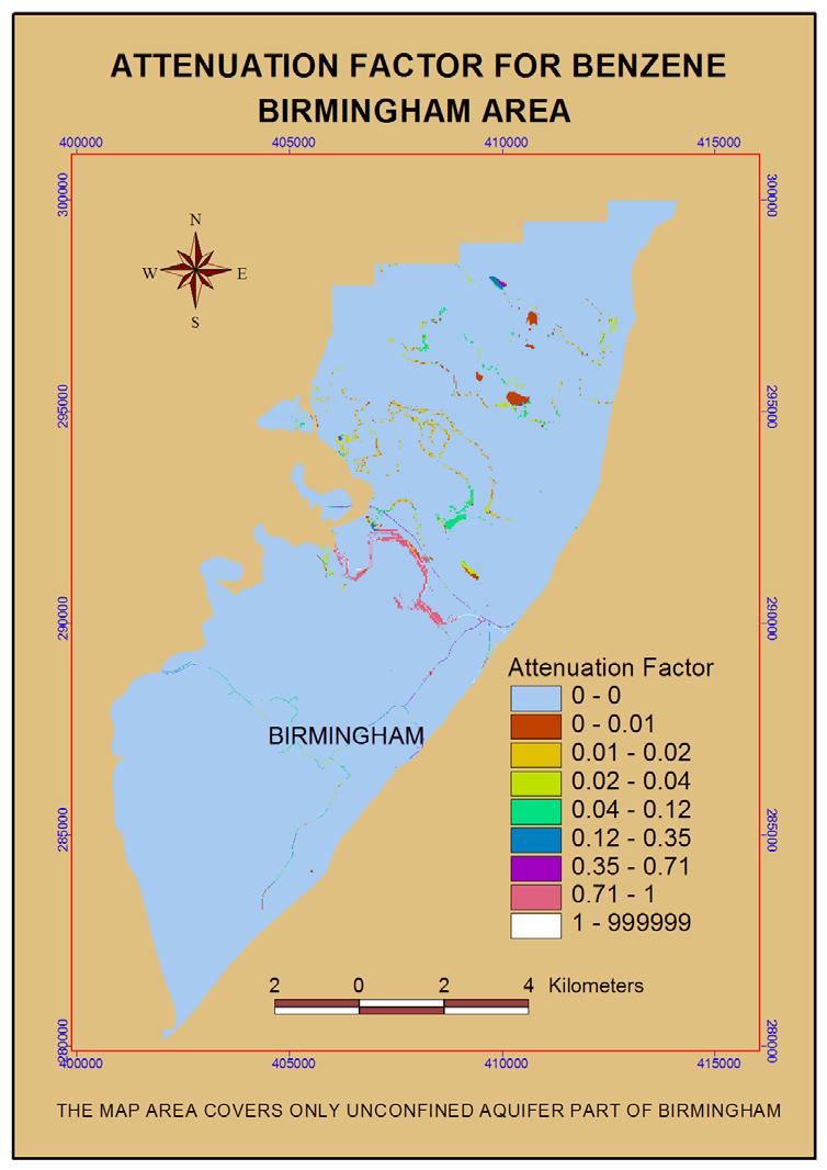
31 The Attenuation Factor Model The Attenuation factor (AF) index denotes mass emission of a chemical from the unsaturated zone to groundwater as: AF = M M Rf θ b d ΚΗ 2 1/2 Rf = [1+ + ] 1 = exp qt z M1 = initial mass of chemical applied at the ground surface M2 = mass of chemical exiting the vadose zone. T1/2 = the half life period; λ = first order degradation rate coefficient for the chemical. Rf = Retardation factor. Rf = 1 + (ρbkd + (θs - θ) KH) / θ ρb is the bulk density of the soil; ε = air-filled porosity, θ is the volumetric water content of the soil; θs is the saturated water content of the soil on a volume basis; Kd = Koc foc which is the partition coefficient for the pollutant in the soil; KH is the dimensionless value of Henry s law constant. Here Rf includes the effects of soluble-vapour phase distribution. ρ K θ ε θ

32 Leaching Potential Index (LPI) Model It is a methodology for ranking sites on the basis of their susceptibility to groundwater contamination. This method is a simplification of one dimensional mass balance equation for the convective transport-dispersion-reaction process of solutes in a homogeneous porous medium. Assuming steady state conditions and negligible dispersion, Meeks and Dean (1990) simplified the mass balance equation as: C C 2 1 = M M 2 1 = exp R f qt z 1/2 θ LPI = q 1000[ θ ( )R T1/ is a constant that converts the LPI into a practical range. The term within the parenthesis is an indication of the vulnerability of a site. High values indicates greater susceptibility to contamination. f ] z

33

34 Ranking Index Model Ranking Index model is a methodology developed by Britt et al. (1992) for streamlining the pesticide registration and approval program of the Florida Department of Agricultural and Consumer Service, USA. The ranking index (RI) for a chemical denotes the vulnerability to groundwater contamination by that compound. RI is expressed as: RI = R [ q ( )T1 / θ This model requires setting up of a threshold value for RI (e.g. 500); thus a chemical with an RI of 500 or higher value for a particular site was considered for registration. If the RI is less than 500, then a complete analysis involving studies on leaching, adsorption/desorption, hydrolysis, soil dissipation, and groundwater monitoring is required for registration. f 2 z ]

35 Vulnerability of Conservative Contaminants Assessment of intrinsic vulnerability of conservative contaminants can be done based on the evaluation of vertical travel time from the land surface to the aquifer. Travel time through the vadose zone can be calculated using the simple formula: T time = z θ Vd Where T time is travel time in years, z = vadose zone depth (m), θ = average moisture content or volumetric water content and V d is average recharge rate (m/day). A similar approach has been be undertaken in Poland by Andrzej et al, 2004.

36

37 THANK YOU VERY MUCH