William K. Jaeger, Oregon State University FEEM, Venice, December 9, 2010

Transcription

1 William K. Jaeger, Oregon State University FEEM, Venice, December 9, 2010 Collaborators: Van Kolpin, University of Oregon Ryan Siegel, Oregon State Univ.

2 Today s Agenda Emphasis on empirical issues Brief review of issue, theory Data issues Newly compiled data Preliminary results Discussion

3 The proposition that there may be a U-shaped path (or inverted U-shaped path ) for the environment with rising income per capita Several theoretical models indicate this is possible Evidence is mixed; many observers skeptical.

4 Sketch of theory: from THE ENVIRONMENTAL KUZNETS CURVE FROM MULTIPLE PERSPECTIVES William K. Jaeger and Van Kolpin* April 3, 2008 (Also a FEEM Working Paper from April 2008 Similar mathematically to Stokey (1998); also John and Pecchino (1994), Seldon and Song (1995) Key elements: Endowment of environmental quality is initially relatively abundant compared to income and commodities Growth in income enables greater consumption relative to (diminished) environmental quality The possibility of a turning point depends on the substitutability in preferences and in production technology

5 Intuition for EKC possibility Figure 3. Efficient allocation of an environmental endowment at various income levels E Indifference curve PPF 1 e PPF 2 PPF 6 PPF 3 PPF 4 PPF 5 c, per capita consumption

6 Figure 1. PPF expansion: Indifference curve I 2 is less steep than P(y 1 ) at the level of environmental quality e 0. E I 2 I 3 e 1 I 1 e 0 P(y 0 ) P(y 1 ) c 0 c 1

7 Basic model: x 1 and x 2 represent levels of inputs 1 and 2 The per capita production function is c=c(x 1,x 2 ) where c(x 1,x 2 ) represents the quantity of private good Environmental quality is e=e-d(nx 1 ), where E represents the initial endowment of environmental quality, n is the population size, and d represents a differentiable, increasing, and convex environmental degradation function. Each agent s budget constraint is x 1 +x 2 =y; where y is per capita income.

8 General findings: THEOREM 1: A parametric change will increase optimal environmental quality if and only if the change increases production elasticity relative to consumption elasticity at the initially optimal environmental quality level. Theorem is applied to three different models

9 CES Version of the model We assume both production and utility functions are CES: Let c(x 1,x 2 ) = (a 1 x α 1 + a 1 x α 2 ) 1/α and u(c,e)= (b 1 c β + b 2 e β ) 1/β where α,β 1, α,β 0, and a 1,a 2,b 1,b 2 > 0. this model is symmetric in both production and utility; production is homothetic in x 1 and x 2, and utility is homothetic in c and e.

10 Results for CES model with rising income per capita By Theorem 1 we may conclude the income trajectory of e must be eventually increasing whenever β <α, or equivalently, whenever the elasticity of substitution in the production function (i.e., 1/(1 α)) exceeds the corresponding elasticity of substitution in the utility function (i.e., 1/(1 β)).

11 Results for CES model with rising population (holding income per capita fixed) If both functions reflect CES substitution possibilities that are inelastic, (i.e., α,β <0), then this implies consumption elasticity exceeds production elasticity in the limit it follows environmental quality must be eventually decreasing. in all other cases, environmental quality must be eventually increasing.

12 Is there intuition for the population results? Population growth and the trajectory of optimal environmental allocations MB, MC MB 2 MC 2 MB 1 MC 1 Pollution/environmental damage Q* Abatement

13 Population growth and the trajectory of optimal environmental allocations MB, MC MC 3 MB 3 MB 2 MC 2 MB 1 MC 1 Pollution/environmental damage Q* Abatement

14 Population growth and the trajectory of optimal environmental allocations MB, MC MC 4 MC 3 MB 3 MB 4 P* MB 2 MC 2 MB 1 MC 1 Pollution/environmental damage Q* Abatement

15 Observations from theory Results suggest the possibility of an EKC without making heroic assumptions The production possibilities frontier incorporates whatever influences a government or other coordinating institution is capable of exerting. Parameters in both utility and production will vary by pollutant and community.

16 Empirical evidence Many studies, no consensus, much controversy: Recent survey: R. Carson, The Environmental Kuznets Curve: Seeking Empirical Regularity and Theoretical Structure Review of Environmental Economics and Policy, volume 4, issue 1, winter 2010, pp Stern, D.I. (2004), The Rise and Fall of the Environmental Kuznets Curve, World Development, 32, Marzio Galeotti, Matteo Manera & Alessandro Lanza, On the Robustness of Robustness Checks of the Environmental Kuznets Curve, FEEM Working Paper

17 From Richard Carson, REEP 2009: On the main message taken from Grossman and Krueger s work by the economics profession that trade and higher income levels would make for a better environment the supporting evidence is scant, fleeting, and fragile. Desperately sought, causality has yet to be conclusively found.

18 Empirical issues (air pollution): Most studies have used GEMS/AIRS data, but its data quality is questionable GEMS was discontinued by UNEP in early 1990s. In many cases, data for a city has been combined with country-level values for income per capita and, in some cases, land area (to compute population density) Estimation issues: model specification questions

19 UNITED NATIONS ENVIRONMENT PROGRAMME ENVIRONMENTAL OBSERVING AND ASSESSMENT STRATEGY REFERENCE PAPER ANNEXES REVIEW OF PAST ACTIVITIES, PRESENT GAPS AND LESSONS LEARNED The USEPA donated database, software, maintenance, and other labour to provide a home and distribution center for GEMS/Air data. USEPA rarely received data directly from the 48 participating GEMS countries. Instead this data passed through the GEMS/AIR office of WHO in Geneva. GEMS/Air has never received data from the vast bulk of air quality monitoring stations in the world.. As a result, the GEM/AIR database cannot provide answers to many pertinent questions about trends in global air quality or the extent of exposed populations. In addition, there does not appear to have been quality control efforts, such as inter-calibration of equipment, to insure comparability of data among countries.

20 Objectives and focus of current study: Acquire data for sites with site-specific environmental, income and population density data Include the largest possible sample across geographical units and years So far, sources are concentrated in USA, Europe, Canada

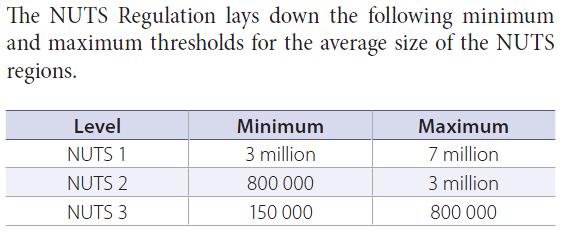
21 Data from Europe The NUTS classification is a hierarchical system for dividing up the economic territory of the EU for the purpose of : The collection, development and harmonisation of EU regional statistics. Socio-economic analyses of the regions. LEVELS: NUTS 1: major socio-economic regions NUTS 2: basic regions for the application of regional policies NUTS 3: as small regions for specific diagnoses

22 NUTS Levels

23

24

25 Main data sources Economic data: Eurostat NUTS-3 US Bureau of Economic Analysis, NOAA CANSTAT Environmental data EU AirBase (SO2, PM10, others) US EPA AirData (SO2, PM10,, others) NAPS (SO2) (Canada)

26 Compiling EU AirBase data Pull all SO2, PM10 data for all stations, years Use latitude and longitude in ArcGIS to overlay with NUTS-3 regions. Use filters to select background stations (omit some stations such as traffic, industry, other) Compute mean values by year for each NUTS-3 region Combine with data on income, pop. for each NUTS-3

27 Table 1. Data Comparisons for SO2 Estimations Harbaugh, Levinson, Lewis* Antweiler, Copeland, Taylor* Current Study Grossman & Krueger* Number of observations 21,298 1,352 2,401 2,555 Number of countries Number of localities Years (maximum by country) Income per capita -- mean 26,200 12,617 15,842 14,780 Income per capita -- minimum 1,800 1,040 1,285 1,090 Income per capita -- maximum 184,860 29,064 30,408 27,180 Pop. density - mean (pers/km2) Pop. density - min (pers/km2) Pop. density - max (pers/km2) 27, * Income per capita, and in some cases population density, are not site specific; but based on national values.

28 From Harbaugh et al.

29 Reduced form model SSSS 2 = αα + ββ 1 YY + ββ 2 YY 2 + ββ 3 YY 3 + ββ 4 PP + ββ 5 PP 2 + ββ 6 PP 3 + ββ 7 TT + εε Where: Y = income per capita, moving average for t and previous 5 years P = population density, persons/km 2 T = trend (year)

30 Table 2. Results for SO2 model estimations Model 1: Fixed effects, smoothed pop. Model 2: Random effects estimator Model 3: pop-avg. est., year dummies Independent variables Coeff. Std. error sig. Coeff. Std. error Coeff. Std. error Coeff. Std. error Income per capita, moving avg. (t-5 to t) ** *** *** *** Income (ma)^ *** *** *** *** Income (ma)^ ** *** *** *** Population density *** 2.56E E-04 *** *** *** Pop density^ *** -2.33E E-08 *** *** *** Pop density^3 1.06E E-03 *** 6.92E E-12 *** 1.04E E-03 *** 4.22E E-03 *** Year *** E-03 *** *** *** Intercept *** *** *** *** # of observations # of groups R^2 (within) Hausman chi^ Model 4: pop-avg. estimator, weighted

31

32

33 Discussion Empirical issues Data quality from GEMS Use of national values for income per capita Misspecification and population density Lags and asymmetry of causal relationships Conceptual issues Theory is robust as a possibility No basis to expect uniformity across pollutants Too much focus on the turning point Most studies find a declining trend this is important!