Underground pumped storage hydroelectricity using abandoned works (deep mines or. /

Transcription

1 1 2 Underground pumped storage hydroelectricity using abandoned works (deep mines or open pits) and the impact on groundwater flow Estanislao Pujades 1, Thibault Willems 1, Sarah Bodeux 1 Philippe Orban 1, Alain Dassargues 1 1 University of Liege, Hydrogeology & Environmental Geology, Aquapole, ArGEnCo Dpt, Engineering Faculty, B52, 4000 Liege, Belgium Corresponding author: Estanislao Pujades 14 Phone: Fax: estanislao.pujades@ulg.ac.be / estanislao.pujades@gmail.com

2 Abstract Underground pumped storage hydroelectricity (UPSH) plants using open-pit or deep mines can be used in flat regions to store the excess of electricity produced during lowdemand energy periods. It is essential to consider the interaction between UPSH plants and the surrounding geological media. There has been little work on the assessment of associated groundwater flow impacts. The impacts on groundwater flow are determined numerically using a simplified numerical model which is assumed to be representative of open-pit and deep mines. The main impact consists of oscillation of the piezometric head, and its magnitude depends on the characteristics of the aquifer/geological medium, the mine and the pumping and injection intervals. If an average piezometric head is considered, it drops at early times after the start of the UPSH plant activity and then recovers progressively. The most favorable hydrogeological conditions to minimize impacts are evaluated by comparing several scenarios. The impact magnitude will be lower in geological media with low hydraulic diffusivity. However, the parameter that plays the more important role is the volume of water stored in the mine. Its variation modifies considerably the groundwater flow impacts. Finally, the problem is studied analytically and some solutions are proposed to approximate the impacts, allowing a quick screening of favorable locations for future UPSH plants Keywords: Energy Storage, Mining, Hydroelectricity, Numerical modeling 2

3 39 1. Introduction The best option to increase the efficiency of energy plants consists of adjusting the energy generated to the demand. Nuclear energy plants produce a relatively constant energy amount as a function of time, while wind and solar technologies produce energy during time intervals that do not specifically correspond to consumption periods. Pumped storage hydroelectricity (PSH) plants are an alternative way to increase efficiency because they store energy by using the excess of produced electricity. PSH plants consist of two reservoirs of water located at different heights (Steffen, 2012). During periods of low demand, the excess of electricity is used to pump water from the lower reservoir into the upper reservoir, thus transforming electric power into potential energy. Afterwards, during peak demand periods, water is released from the upper to the lower reservoir to generate electricity (Hadjipaschalis et al., 2009, Alvarado et al., 2015). More than 70% of the excess energy generated by conventional plants can be reused via PSH plants (Chen et al., 2009). PSH plants cannot be constructed in flat areas and are commonly placed in mountainous regions. Their construction often generates controversy due to the effects on the land use, landscape, vegetation and wildlife caused by the reservoirs (Wong, 1996). These are not negligible because of the large dimensions of the considered reservoirs, which are usually large to increase the amount of stored energy. Underground pumped storage hydroelectricity (UPSH) could be an alternative means of increasing the energy storage capacity in flat areas where the absence of mountains does not allow for the construction of PSH plants (reservoirs must be located at different heights requiring location in mountainous regions). UPSH plants consist of two reservoirs, with the upper one located at the surface or possibly at shallow depth underground while the lower one is underground. These plants provide three main benefits: (1) more sites can be considered in comparison with PSH plants (Meyer, 2013), (2) landscape impacts are smaller 3

4 than those of PSH plants, and (3) the head difference between reservoirs is usually higher than in PSH plants; therefore, smaller reservoirs can generate the same amount of energy (Uddin and Asce, 2003). Underground reservoirs can be excavated or can be constructed using abandoned cavities such as old deep mines or open pits. The former possibility has been adopted to increase the storage capacity of lower lakes at some PSH plants (Madlener and Specht, 2013) and allows full isolation of the lower reservoir mitigating the interaction between the used water and the underground environment. While the reuse of abandoned works (deep mines or open pits) is cheaper, the impacts on groundwater can be a problem. Consequently, the interaction between UPSH plants and local aquifers must be considered to determine the main impacts of such a system. Any detailed studies on this interaction have not been published before. In theory, two impacts are expected from the interaction between UPSH plants and groundwater: (1) alteration of the piezometric head distribution in the surrounding aquifer, and (2) modification of the chemical composition of the groundwater. This paper is focused only on the groundwater quantity issue (1). Piezometric head modifications may have negative consequences. Lowering of heads can cause the drying of wells and springs, death of phreatophytes, seawater intrusion in coastal aquifers and ground subsidence (Pujades et al., 2012). Rising water levels may provoke soil salinization, flooding of building basements (Paris et al., 2010), water logging, mobilisation of contaminants contained in the unsaturated zone and numerous geotechnical problems such as a reduction of the bearing capacity of shallow foundations, the expansion of heavily compacted fills under foundation structures or the settlement of poorly compacted fills upon wetting (Marinos and Kavvadas, 1997). Therefore, it is of paramount importance to determine the following: (1) what are the main impacts caused by UPSH plants on the groundwater flow, and (2) what is the role of the aquifer and mine characteristics on the impacts? Understanding these will help us to select the best places to locate future UPSH plants. In the same way, it will be very useful to provide 4

5 simple analytical solutions for rapidly estimating the main trend of possible impacts. This will allow for screening many potential UPSH locations in a short time. After this first screening, detailed numerical models will still be necessary to describe the details of a planned UPSH plant and its impacts before making the definitive choice and beginning construction. Numerical modelling is used for studying several scenarios varying (1) the hydrogeological parameters of the aquifer, (2) the properties of the underground reservoir, (3) the boundary conditions (BCs), and (4) the characteristic time periods when the water is pumped or released. Simulation of a UPSH plant based on real curves of electricity price is also modelled. Analytical procedures are proposed based on existing hydrogeological solutions that estimate the groundwater flow impacts of a theoretical UPSH lower reservoir Problem statement The geometry of real deep or open pit mines may be complex. Deep mines have numerous galleries and rooms, while open pit mines have irregular shapes. Given that the objective is to determine and study the main impacts in the surrounding aquifer, the geometry of the underground reservoir (mine or open pit) is simplified here: a square underground reservoir (plan view) is considered in unconfined conditions, with a thickness of 100 m (Figure 1). The thickness of the underground reservoir is the same as that of the aquifer. The geometrical simplification is required to reach general and representative results that can be useful in case of deep and open pit mines. If a system of horizontal galleries had been modelled, results would not been suitable for open-pit mines or deep mines with galleries at different depths. However, previous studies have proved that a complex deep mine can be discretized using a single mixing cell and modelled as a single linear reservoir characterised by a mean hydraulic head (Brouyère et al., 2009, Wildemeersch et al., 2010). In addition, groundwater response to pumping in radial collector wells, that can be considered as similar 5

6 to deep mines, is fully similar to the response produced by a single vertical well with an equivalent radius (Hantush, 1964). The considered aquifer is homogeneous although real underground environments are heterogeneous (vertically and horizontally). This choice is adopted to obtain general and representative solutions. However, results can be extrapolated to heterogeneous underground environments adopting effective parameters. This procedure has been previously used by several authors obtaining excellent results (e.g. in Pujades et al., 2012). The water table is assumed initially at 50-m depth everywhere in the modelled domain. Piezometric head evolution is observed at 50 m from the underground reservoir at two depths: at the bottom of the aquifer and just below the initial position of the water table. These two points are selected considering the delayed water table response in unconfined conditions (explained below). The maximum early groundwater response to pumping or injection in the system cavity is observed at the bottom of the geological medium while the minimum groundwater response is observed at the top of the saturated zone. Therefore, these two points show the maximum and minimum groundwater flow impacts. Groundwater flow exchanges between mines and surrounding aquifers depend on the properties of the mine walls. These can be lined with low hydraulic conductivity materials (concrete) in deep mines or can remain without treatment in case of open-pit mines. Different lining conditions are considered to ascertain their influence on the groundwater flow impacts. External boundaries are located at 2500 m from the underground reservoir. The duration of any pumping/injection cycle is always 1 day, but two types of pumping/injection cycles are considered: regular and irregular. Cycles are regular when (1) the pumping and injection rates are the same, (2) they are consecutive, and (3) they have the same duration (0.5 days). Cycles are irregular when the injection rate is higher. As a result, if there is no external contribution of surface water, pumping takes more time and there is a no-activity period during each cycle. The pumping and injection rates are 1 m 3 /s when 6

7 regular cycles are considered, while irregular cycles are simulated with pumping and injection rates of 1 and 2 m 3 /s, respectively. Pumping lasts 0.5 days and injection 0.25 days Numerical study 3.1. Numerical settings The finite element numerical code SUFT3D (Brouyère et al., 2009 and Wildemeersch et al., 2010) is used to model the unconfined scenarios. This code uses the control volume finite element (CVFE) method to solve the groundwater flow equation based on the mixed formulation of Richard s equation proposed by Celia et al. (1990): 151 K h K z q t (1) where is the water content [-], t is the time [T], K is the hydraulic conductivity tensor [LT -1 ], h is the pressure head [L], z is the elevation [L] and q is a source/sink term [T -1 ]. The used mesh is made up of prismatic 3D elements and is the same in all scenarios. The domain is divided vertically into 16 layers. The thickness of the individual layers is reduced near the water table levels. The top and bottom layers are 10-m thick, while layers located near the water table are 1-m thick. The horizontal size of the elements is 500 m near the boundaries and 10 m in the centre of the domain (Figure 1). The vertical and horizontal discretization and the number of layers are adopted/optimised to reduce the convergence errors. The used mesh allows for reducing these errors to less than m, which is the chosen value for the convergence criteria. The underground reservoir is discretized as a single mixing cell and modelled as a linear reservoir. Groundwater exchanges vary linearly as a function of the water level difference between the reservoir and the surrounding porous medium (Orban and Brouyère, 2006). An internal dynamic Fourier boundary condition (BC) between the underground 7

8 reservoir and the surrounding aquifer (Wildemeersch et al., 2010) is used to simulate the groundwater exchanges. The internal Fourier BC is defined as follows: i aq ur Q A h h (2) where Q i is the exchanged flow [L 3 T -1 ], h is the piezometric head in the aquifer aq [L], h ur is the hydraulic head in the underground reservoir [L], A is the exchange area [L 2 ] and is the exchange coefficient [T -1 ]. K b where K and b are the hydraulic conductivity [LT -1 ] and the width [L] of the lining, respectively. Different lining conditions are considered varying the value of. Low values of simulate lined walls while no lined walls are characterised by high values of. The internal Fourier boundary condition assumes that groundwater flow exchanges occur in a uniformly distributed manner, which is not always true. Therefore, results must be carefully considered when groundwater flow exchanges occur locally. Given that the underground reservoir is characterised by means of a single mixing cell, groundwater is pumped from (or injected through) all the saturated thickness of the reservoir. Figure 1 shows the main characteristics of the numerical model. (Yeh, 1987): The retention curve and the relative hydraulic conductivity are defined as follows K r s r hh r a hb ha r s r (3) (4) 184 where s is the saturated water content [-], r is the residual water content [-], K r 185 is the relative hydraulic conductivity [LT -1 ], h b is the pressure head at which the water content is the same as the residual one [L], and content is lower than the saturated one [L]. h a and h a is the pressure head at which the water h b are taken as 0 and -5 m (not modified in any scenario). The applied law to define the transition between the partially saturated and 8

9 the saturated zones is chosen for its linearity: (1) it does not affect the results of this study, which are focused on the saturated zone, and (2), it allows for elimination of convergence errors that can appear using other laws. Several scenarios are modelled to determine the influence of different parameters on the calculated piezometric head evolution. One variable is modified in each set of simulations to establish its influence on the groundwater flow impact. Variables assessed include the aquifer parameters (hydraulic conductivity and saturated water content), the underground reservoir attributes (exchange coefficient and underground reservoir volume), the type of BCs and the pumping and injection characteristics. Table 1 summarizes the parameters of each scenario. To consolidate and clarify Table 1, all variables are only specified for Scenario 1 (Sce1) and only the variable modified (and its value) with respect to Sce1 is indicated for the other scenarios. Sce1 is the reference scenario with regular cycles and its characteristics are as follows: K, s and r are 2 m/d, 0.1 and 0.01, respectively. Although these values are representatives of real aquifers, the objectives had been also reached using others parameters. The objective is not to compute the groundwater flow impact in a given aquifer. The goal is to define the general characteristic of the groundwater flow impacts and assess the influence on them of several parameters. No lining is regarded in Sce1, therefore, the exchange coefficient (α ) considered in the Fourier exchange fluxes is high (α =100 d -1 ). External boundaries are taken far enough (2500 m) for not biasing results during pumpings and injections (i.e. farther than the influence radius) and a null drawdown can be assumed on them. Therefore, in Sce1 a Dirichlet BC consisting of a prescribed piezometric head at 50 m (the same as the initial head) is applied. In other scenarios, boundaries are also moved closer to the underground reservoir and the BCs are modified to assess their influence on the groundwater flow impacts Numerical results 9

10 General piezometric behavior Piezometric head evolution in the surrounding aquifer is computed for Sce1 considering regular cycles (Figures 2a, 2b and 2c). Numerical results are calculated at an observation point located at 50 m from the underground reservoir. Figure 2a displays the computed piezometric head evolution over 500 days at two different depths: at the bottom of the aquifer (100-m depth) and below the initial position of the water table (55-m depth). Figures 2b and 2c show in detail the computed piezometric head evolution at the bottom of the aquifer during early and late simulated times, respectively. Groundwater oscillates in the porous medium consequently to the water pumping and injection into the cavity. Initially, hydraulic head in the underground reservoir is the same as the piezometric head in the aquifer. When water is pumped, the hydraulic head in the underground reservoir decreases rapidly producing a hydraulic gradient between the aquifer and the reservoir. As a result, groundwater seepage creates an inflow into the reservoir reducing the piezometric head. In contrast, when water is injected, it is creating a rapid increase of the hydraulic head in the underground reservoir that is higher than the piezometric head in the surrounding medium. Therefore, water flows out increasing the piezometric head in the aquifer. The groundwater response to the continuous alternation of pumping and injection causes the piezometric head oscillations in the porous medium. The average head ( h ), maximum drawdown and oscillation magnitude are important for groundwater impact quantification. h is the head around which groundwater oscillates: it is computed from the maximum and minimum heads of each cycle. h increases after the drawdown occurred at early simulated times and reaches a constant value ( h SS ) when a dynamic steady state is achieved. In the simulated scenario, h SS is the same as the initial piezometric head of the aquifer. Maximum drawdown occurs during early cycles, and it is caused by the first pumping. However, the cycle when the maximum drawdown is observed depends on the aquifer parameters as well as on the distance between the underground 10

11 reservoir and the observation point because the maximum effect of the first pumping is delayed at distant points. Maximum drawdown is only observed during the first cycle close to the underground reservoir. The delayed time at a distant point can be easily calculated from Eq. 5, 245 t D 2 SLOBS (5) T where t D is the delayed time [T], S is the storage coefficient of the aquifer [-], L OBS is the distance from the underground reservoir to the observation point [L] and T is the transmissivity of the aquifer [L 2 T -1 ]. The delayed time in Sce1 for an observation point located at 50 m from the underground reservoir is 2.5 days. This agrees with the cycle where the maximum drawdown is observed (see Figure 2). Groundwater behaves quasi-linearly during pumping and injection periods given the large water volume stored in the underground reservoir and the short duration of pumping and injection periods. Most of the pumped water is stored in the underground reservoir, but a relatively small percentage inflows from and flows out towards the surrounding aquifer. These groundwater exchanges produce head increments inside the underground reservoir and therefore in the surrounding aquifer at the end of the first cycles (Figure 2b). The magnitude of these piezometric head increments decreases with time until a dynamic steady state is reached. Piezometric head evolution depends on depth. The computed oscillation magnitude and maximum drawdown are lower at shallower depths. This behaviour is associated with the fact that the delayed water table response in unconfined aquifers is most pronounced at the bottom of the aquifer (Mao et al., 2011). During early pumping times, drawdown 263 evolution at the bottom agrees with the Theis solution with S S b (Neuman, 1972). In S contrast, at the water table, drawdown is more similar to the Theis curve (Stallman, 1965) with SSb S Sy, where S y s is the specific yield (Figure 3). As a result, the early 11

12 groundwater response to pumping or injection increases with depth, since SS Sy. This fact can be deduced from transient groundwater flow equations such as Thiem or Jacob s equations. Differences between the piezometric head computed at the bottom and the top of the saturated zones increase close to the underground reservoir (Neuman, 1972) Influence of aquifer parameters Numerical results for different scenarios computed at 50 m from the underground reservoir are compared to determine the influence of the aquifer parameters on the groundwater flow. Figures 4a and 4b display the computed piezometric head evolution during 500 days at the bottom and at the top of the aquifer, respectively, assuming hydraulic conductivity values of 2 m/d (Sce1), 0.2 m/d (Sce2) and 0.02 m/d (Sce3). The oscillation magnitude decreases logically when K is reduced. This effect is more perceptible at the top of the saturated zone. Similarly, the maximum drawdown also decreases when K is reduced. The reduction of oscillation magnitude and maximum drawdown with lower values of K is a consequence of the groundwater evolution in transient state. The affected area by pumping or injection during 0.5 days decreases with lower values of K. This distance can be computed applying Eq. 5, replacing L OBS by the affected distance of the aquifer by a pumping (or injection) event and t D by the pumping time. Therefore, if the K of the aquifer is increased, the affected area increases, producing drawdown (or higher drawdown) at locations which would not be affected (or would be less affected) with lower values of K. However, low values of K increase the time needed to reach a dynamic steady state ( t SS ). As a result, the piezometric head is located above the initial point for a longer time. In fact, h cannot be SS compared because a dynamic steady state is not reached for Sce2 and Sce3. However, it is possible to deduce from the following simulations that K does not affect h SS. Note that the 12

13 groundwater flow impact observed at the top of the aquifer when the dynamic steady state is reached will be negligible if K is low (Sce3). The influence of S on the groundwater flow impact in the surrounding aquifer is computed by modifying s because S SSbSy Sy s. Figures 4c and 4d show the computed piezometric head evolution at 50 m from the underground reservoir at the top and at the bottom of the saturated zone, respectively. Three scenarios are compared: s = 0.1 (Sce1), s = 0.2 (Sce4) and s = 0.05 (Sce5). There is not a significant change in the time needed to reach a dynamic steady state. The influence of s on t SS is analysed analytically and explained below (see section 4.2.3). s affects the oscillations magnitude and the maximum drawdown more. These are smaller when s is increased because higher values of s soften the response of the surrounding aquifer in terms of piezometric head variation. In other words, higher values of s require less drawdown to mobilize the same volume of groundwater, reducing the aquifer response to each pumping and injection. h is equal for SS the three scenarios. Computed piezometric head evolution varies more at the top than at the bottom of the saturated zone when s is modified. This fact confirms that S depends on (1) S y at the top of the saturated zone and (2) SS at the bottom of the aquifer. It is possible to conclude from the results obtained in this section that the impact on groundwater increases with the value of the hydraulic diffusivity of the aquifer (T/S). As a result, impacts will be higher in high-transmissive aquifers, and specifically, in confined high-transmissive aquifers characterized by a low storage coefficient Influence of reservoir characteristics The size of the underground reservoir is important to the impact on groundwater flow. Its influence is evaluated by reducing the volume of the reservoir by a factor of

14 (Sce6) but keeping the same pumping and injection rates. Figures 5a and 5b display the computed piezometric head evolution at 50 m from the underground reservoir for Sce1 and Sce6. Figure 5a displays the computed piezometric head at the bottom of the aquifer, while Figure 5b shows the computed piezometric head at the top of the saturated zone. As expected, if the volume of the underground reservoir is reduced and the pumping and injection rates stay the same, the oscillation magnitude and maximum drawdown increase. Although the magnitude of oscillations is higher for Sce6, h is logically the same in both SS scenarios once the dynamic steady state is reached. Significant changes for t SS are not appreciated because the effects of modifying the radius of the underground reservoir are opposite. On the one hand, t SS is lower if the size of the reservoir is reduced because less groundwater flows into the underground reservoir to increase its hydraulic head. On the other hand, t SS is higher because the contact surface between the surrounding aquifer and the underground reservoir decreases when the radius of the underground reservoir is reduced. As a result, the maximum inflow rate decreases. The influence of the underground reservoir size on t SS is evaluated analytically below. Groundwater flow impact is computed by varying exchange coefficient between the underground reservoir and the aquifer (α ). For the reference scenario (Sce1), α is set large enough (100 d -1 ) to ensure that water inflows and outflows are not significantly influenced (Willems, 2014). α implemented for Sce7 and Sce8 are 1 and 0.1 d -1, respectively. Figures 5c and 5d display the computed piezometric head evolution at 50 m from the underground reservoir for the three scenarios. The computed piezometric head at the bottom of the aquifer is displayed in Figure 5c, while Figure 5d shows the computed piezometric head at the top of the saturated zone. The oscillation magnitude and maximum drawdown decrease when α is lower, while h is the same for the three scenarios. Differences in SS t SS are not appreciable. The influence of α is expected to be similar to that of K. Low values of α reduce the 14

15 hydraulic connectivity between the underground reservoir and the surrounding aquifer, therefore reducing the groundwater inflow. As a result, more time is needed to increase the average hydraulic head inside the underground reservoir and reach a dynamic steady state Influence of boundary conditions (BCs) The influence of the lateral BCs on the groundwater flow impact was also assessed. Dirichlet BCs are assumed for the reference scenario (Sce1), no-flow BCs for Sce9 and Fourier BCs with a leakage coefficient (α=0.005 d -1 ) for Sce10. The size of the aquifer is reduced (500x500 m) to better observe the influence of the boundaries. Simulated pumping- injection cycles are regular. Figures 6a and 6b display computed piezometric head evolution at 50 m from the underground reservoir for Sce1, Sce9 and Sce10. Computed piezometric head evolution is shown at the bottom (Fig 6a) and at the top (Fig 6b) of the saturated zone. Given that variations are hard to distinguish, the computed piezometric head for Sce1 is subtracted from those computed for Sce9 and Sce10 to detect the influence of the lateral BCs (Figure 6c). The oscillation magnitude and maximum drawdown tend to increase with low α Fourier BCs and no-flow BCs. These increments are maximum if BCs are no-flow (Figure 6c). Although h differs at early simulated times, it is the same for Sce1 and Sce10 and lower for Sce9 once the dynamic steady state is reached. Fourier BCs allow groundwater to flow through the boundaries. Therefore, the maximum h, during the dynamic steady state, is the same as with Dirichlet BCs (Figure 6c). However, the time to reach a dynamic steady state is different. This time increases for low α Fourier BCs. In contrast, impervious boundaries do not provide any groundwater to the aquifer. As a result, h is below the initial head and SS the dynamic steady state is reached earlier. The piezometric head difference between Sce1 and Sce9 (Figure 6c) increases until reaching a maximum that depends on the storage capacity of the aquifer. The difference will be lower (even negligible) for large aquifers with high S. 15

16 Actual aquifers may be delimited by different BCs. Thus, BCs are combined in Sce11 and Sce12, and the results are compared with those computed for Sce1 (Figures 7a and 7b). Three no-flow BCs and one Dirichlet BC are implemented in Sce11. The three impervious boundaries are replaced by Fourier BCs in Sce12 (α=0.005 d -1 ). The location of the BCs adopted and the point where the piezometric head evolution is computed are displayed in Figure 7c. Figures 7a and 7b show the computed piezometric head evolution at 50 m from the underground reservoir at the bottom (Fig 7a) and the top (Fig 7b) of the saturated zone for Sce1, Sce11 and Sce12. The computed piezometric head for Sce1 is subtracted from those computed for Sce11 and Sce12 to detect the influence of the lateral BCs (Figure 7d). The oscillation magnitude and maximum drawdown increase for Sce11 and Sce12. However, h is equal to the initial piezometric head of the aquifer in all scenarios. This SS occurs because at least one boundary can provide groundwater to the aquifer. Computed piezometric head evolutions are only different during the early simulated times. The calculated piezometric head for Sce12 needs less time to reach a dynamic steady state because Fourier BCs provide more water than no-flow ones (Sce11) Influence of the pumping and injection periods Figure 8 compares the computed piezometric head evolution at 50 m from the underground reservoir at the bottom (Fig 8a) and at the top (Fig 8b) of the saturated zone. Regular (Sce1) and irregular (Sce13 and Sce14) cycles are considered. The aquifer parameters and underground reservoir characteristics are the same in all scenarios. The pumping period is identical for Sce1, Sce13 and Sce14, consisting of pumping 1 m 3 /s from the beginning to the halfway point of each cycle. Differences lie in the second half of the cycles. In Sce1, injection starts just after the pumping, at a rate of 1 m 3 /s for 0.5 days. In Sce13, injection starts just after the pumping, at a rate of 2 m 3 /s for 0.25 days. Finally, in Sce14, injection is simulated during the last 0.25 days of each cycle at a rate of 2 m 3 /s. 16

17 The oscillation magnitude is larger for irregular cycles because a smaller volume of water flows out from the underground reservoir if the injection takes only 0.25 days. As a result, the piezometric head increment caused by irregular cycle injections is higher than those produced from regular cycles. However, the increment in the oscillations magnitude is negligible when compared with them. Maximum drawdown is higher in Sce14 (Figures 8c and 8d) because groundwater flows into the underground reservoir after the pumping (during the no-activity period), which increases the groundwater flow impact on the surrounding aquifer. In contrast, injection in Sce13 raises the head rapidly in the underground reservoir exceeding the piezometric head and reducing the volume of groundwater that flows into the underground reservoir. Similarly, h depends on the characteristics of the injection period. In Sce14, the SS head in the underground reservoir is below the initial piezometric head in the surrounding aquifer during the no-activity periods of each cycle. As a result, groundwater flows into the reservoir, increasing h inside the underground reservoir and therefore in the surrounding SS aquifer. Contrary to this, the head in the underground reservoir is above the piezometric head in the surrounding aquifer during no-activity periods of Sce13. Thus, the volume of groundwater that flows into the underground reservoir is lower Test on an actual pumping-injection scenario A one-year simulation based on pumping and injection intervals deduced from actual electricity price curves is undertaken to evaluate if piezometric head evolution is similar to those computed assuming ideal cycles (regular or irregular). Sce1 is considered for the simulation. Three 14-day electricity price curves are used to define the pumping and injection periods (Figure 9). Each curve belongs to one season (winter, summer and spring). The pumping and injection periods for each season are completed by repeating the 14-day curves, and the annual curve of pumping and injection periods is obtained by assuming that 17

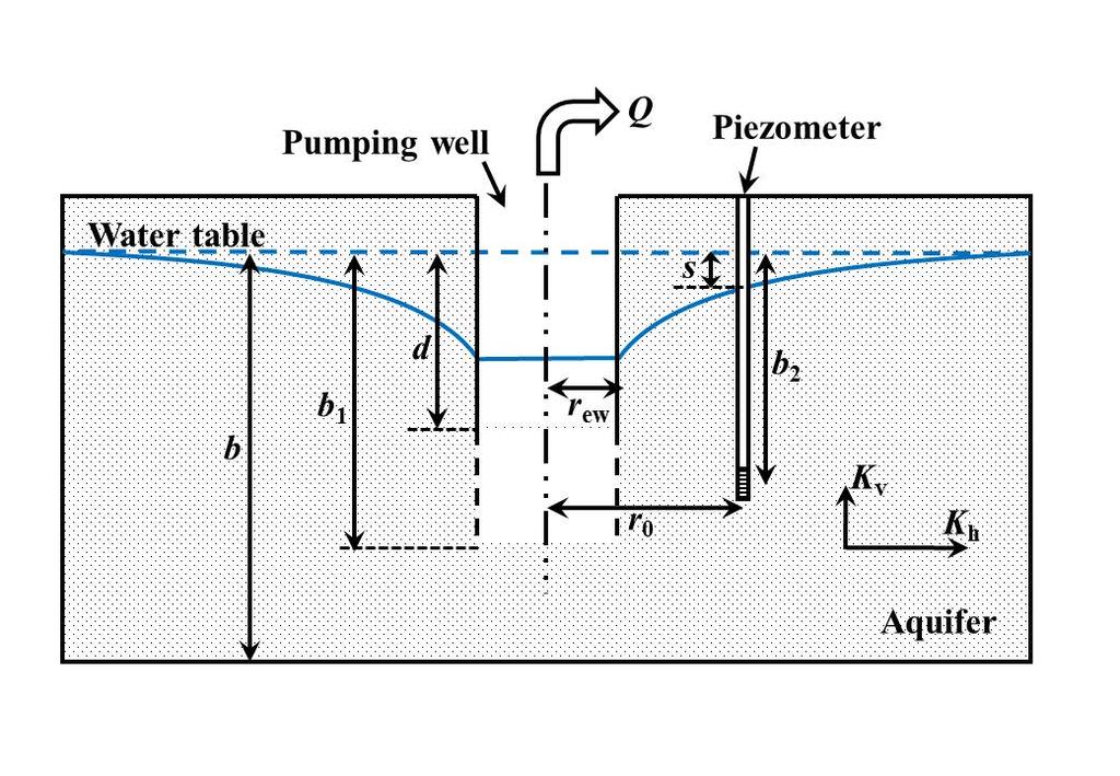
18 the electricity price curve for autumn is similar to that of spring. It is considered that the pumping and injection rates are the same (1 m 3 /s) and that there is not any external contribution of surface water. Figure 10 displays the computed piezometric head at 50 m from the underground reservoir at the top (Fig 10a) and at the bottom (Fig 10b) of the saturated zone. Piezometric head evolution in the surrounding aquifer is similar to that computed assuming ideal cycles. After an initial drawdown, the piezometric head recovers and tends to reach a dynamic steady state. h is stabilized at the end of winter, and it does SS not vary much in spring. However, it increases in the summer and decreases in the autumn. The difference in hss between seasons is related to the pumping and injection characteristics. Intervals between pumping and injection periods are generally longer in summer than in the other seasons (Figure 9), which agrees with the fact that sunset occurs later in summer. Similarly to when irregular cycles are simulated, if the no-activity period between pumping and injection takes more time, more groundwater flows into the underground reservoir. Thus, the average head inside the underground reservoir increases, and h is higher. SS Analytical study 4.1 Analytical settings The underground reservoir can be regarded as a large diameter well if no lining is considered. Therefore, drawdown caused by pumping can be determined analytically using the Papadopulos-Cooper (1967) and Boulton-Streltsova (1976) equations. The Papadopulos- Cooper (1967) exact analytical solution allows for computing drawdown (s) in a confined aquifer: 439 Q s Fu,, r r 4 Kb W 0 ew (6) where b is the aquifer thickness [L], Q is the pumping rate [L 3 T -1 ], r ew is the radius of the screened well [L], and r o is the distance from the observation point to the centre of the 18

19 442 well [L]. WrewS rc, where r c is the radius of the unscreened part of the well [L], and 443 u r S Kbt, where t is the pumping time [T]. It is considered that W S because r c r ew. Values of the function F have been previously tabulated (Kruseman and de Ridder, ) Boulton and Streltsova (1976) proposed an analytical model for transient radial flow (towards a large diameter well) in an unconfined aquifer considering the partial penetration of the well and anisotropy of the aquifer (Singh, 2009). Their solution is only applicable for early pumping times and allows computing drawdown during the first stage of the typical S- shaped response (in a log-log drawdown-time diagram) of an unconfined aquifer (Kruseman and de Ridder, 1994): 452 Q s Fu, S,, ro rew, b1 b, d b, b2 b 4 Kb (7) where b 1 is the distance from the water table to the bottom of the well [L], d is the distance from the water table to the top of the well [L], and b 2 is the distance from the water rb K K, table to the depth where the piezometer is screened [L] (Figure 11). 2 v h where K v and K h are the vertical [LT -1 ] and horizontal [LT -1 ] hydraulic conductivities. These analytical solutions are combined with other ones for determining the mid- term groundwater flow impacts of the repeated cycles. Procedures combined are (1) equations of large diameter wells, (2) methods used to assess cyclic pumpings, and (3) the image well theory (Ferris et al., 1962). Numerous variables are involved in Eq. 7, which makes it difficult to compute function F. As a result, the number of tabulated values is very limited. For this reason, the analytical solutions proposed below are tested using the Papadopulos-Cooper (1967) equation. It is important to remark that results obtained in this section are only useful when groundwater exchanges are not limited by any lining. Therefore, the proposed solutions can be applied in open-pit mines and must be carefully 19

20 applied in lined deep mines. It was considered to use analytical solutions of radial collector wells instead of solutions for large diameter wells. However, the groundwater response to radial collector wells in observation points located further than the maximum distance reached by the radial drains is equivalent to the groundwater response to single vertical wells with an equivalent radius (Hantush, 1964). Given that the goal of this study is to assess impacts in the surrounding aquifer and not in the exploited area, equations for large diameter wells are considered as suitable Analytical results Time to reach a dynamic steady state Figure 2c shows in detail the piezometric head evolution computed numerically for Sce1 once a dynamic steady state is reached. The dynamic steady state occurs when the maximum (or minimum) piezometric heads of two consecutive cycles are the same. Therefore, the difference in the piezometric head between times n and n-1 is 0. Drawdown at n (Eq. 8) and n-1 (Eq. 9) can be written using equations of large diameter wells: Q sn Fn Fn 0.5Fn 1... F1 F 0.5 4T Q sn 1 Fn 1Fn 1.5 Fn 2... F1 F 0.5 4T (8) (9) These equations consider that pumping and injection periods are consecutive and take the same duration (0.5 days). Each function F represents one pumping or injection and depends on the variables shown in Eq. 6 and/or Eq. 7. The number between brackets is the duration (in days) from the start of each pumping or injection event to the considered time when s is computed. These equations become tedious for a great number of cycles because an additional term is required to implement each pumping or injection. Moreover, F must be computed for each pumping and injection because the time changes. Equations are simplified by applying the principle of superposition (Kruseman and de Ridder, 1994) using increments 20

21 of the function F (ΔF) because they are proportional to the drawdown increments. As an example, ΔF considered during the two first regular cycles are shown in Table 2. Drawdown at any time can be easily calculated by adding ΔF from the first pumping and multiplying it by Q 4 Kb. Given that some increments have opposite signs, they will be eliminated to simplify the final equation. Drawdown equations after the first pumping (0.5 days; Eq. 10), the first injection (1 day; Eq. 11) and the second pumping (1.5 days; Eq. 12) can be written using ΔF from Table 2 as follows: 498 s Q F 4T to 0.5 (10) 499 Q s1 F F 0.5 to 1 0 to 0.5 4T (11) 500 Q s1.5 F F F 1 to to 1 0 to 0.5 4T (12) Note that increments of F used in Eq. 12 are those included in the third column of Table 2 but are not being multiplied by 2. For practical purposes, the drawdown equation at any time can be easily written in terms of ΔF following the next steps: 1) Split the function F of a continuous pumping into increments of ΔF. The duration of the increments must be equal to that of the pumping and injection 506 intervals. ΔF must be ordered from late to early times (e.g.,, F 1.5 to 2 days 507,,,.). 0.5 to 1 days 0 to 0.5days F 1 to 1.5days F F ) Change the sign of ΔF (from positive to negative) every two ΔF increments following the ordered list in the previous step. If the first cycle starts with a pumping, change the sign to the ΔF located in even positions (second, fourth, sixth ). In contrast, if the first cycle starts with an injection, change the sign of the ΔF placed in odd positions (first, third, fifth ). 21

22 ) Add all ΔF (considering their sign) from the first pumping until reaching the time when the drawdown has to be calculated and multiply by Q 4 Kb. Thus, the drawdown at times n and n-1, considering that the first cycle starts with a pumping event, is expressed by Eq. 13 and Eq. 14, respectively: Q sn F F F... F F n05 to n n1 to n0.5 (n1) 0.5 to n1 0.5 to 1 0 to T (13) and Q sn 1 F... F F (n1) 0.5 to n1 0.5 to 1 0 to T Dynamic steady state occurs if sn sn 1: (14) 522 F F (15) n0.5 to n n1 to n This takes place when ΔF does not vary (i.e., the slope of F is constant) with radial flow. t SS can be determined by plotting the tabulated values of F versus 1/u and identifying the point from which the slope of F does not vary or its change is negligible. However, this procedure is too arbitrary. Therefore, it is proposed to determine t SS from the derivative of F with respect to the logarithm of 1 u. Flow behaviour is totally radial and dynamic steady state is completely reached when df d respect to log 10 ln 1 u 1 (= 2.3 if the derivative is computed with 1 u ). For practical purposes, it is considered that dynamic steady state is completely reached when df dln1 u 1.1. However, dynamic steady state is apparently reached when the radial component of the flow exceeds the linear one because more than 90% of h is recovered when that occurs. The time when dynamic steady state is apparently reached can be easily determined from the evolution of df d ln1 decreases. As an example, Figure 12 shows df d ln1 u because its value u versus 1 u considering Sce1 for a 22

23 piezometer located at 50 m from the underground reservoir (values of F and u are tabulated in Kruseman and de Ridder, 1994). Flow behaviour is totally radial ( df dln1 u 1.1 ) for 1 u 500, and the percentage of radial flow exceeds the linear one for 1 u 50. More precision is not possible because there are no more available values of F. Actual times are calculated by applying 2 t r0 S 4Kbu. Considering the characteristics of Sce1 (Figure 2a displays the computed piezometric head evolution for Sce1), a dynamic steady state will be completely reached after 1250 days and practically reached after 125 days, which agrees with the piezometric head evolution shown in Figure 2a. Transition from linear to radial flow is observed at different times depending on the location of the observation point. The dynamic steady state is reached before at observation points closer to the underground reservoir. Note that, if the observation point is too far (more than 10 times the radius of the underground reservoir) from the underground reservoir, the slope of F is constant from early times and values of df d ln1 head oscillates around the initial one from the beginning. u do not decrease with time. In these cases, the piezometric This procedure to calculate t SS is only useful if the aquifer boundaries are far enough away so that they do not affect the observation point before the groundwater flow behaves radially. If the boundaries are closer, dynamic steady state is reached when their effect reaches the observation point. This time ( t BSS ) can be calculated from Eq. 16 t BSS 2 L L r0 S (16) T where L is the distance from the underground reservoir to the boundaries [L] Oscillations magnitude 23

24 A solution for estimating oscillations magnitude is proposed by following a similar procedure to that above. Drawdown at time n-0.5 applying the principle of superposition in terms of ΔF is: Q sn0.5 F F... F F (17) n1 to n0.5 (n1) 0.5 to n1 0.5 to 1 0 to T Oscillations magnitude is computed by subtracting drawdown at time n-0.5 (Eq. 17) from drawdown at time n (Eq. 13): Q snsn 0.5 F 2 F 2 F... 2 F 2 F n0.5 to n n1 to n0.5 (n1) 0.5 to n1 0.5 to 1 0 to T (18) Eq. 18 can be simplified assuming that ΔF (and therefore the drawdown) produced by a pumping event is similar to the ΔF caused by an injection started just after (i.e. F F or F F ). Therefore, maximum head n to n0.5 n0.5 to n1 0.5 to 1 0 to 0.5 oscillation ( s ) can be approximated as: 569 Q s F 0 to 0.5 4T (19) It is the same solution as the one used to compute drawdown caused by pumping (or injection) during 0.5 days. If boundaries are too close and can affect the zone of interest, the oscillations magnitude must be calculated using Eq. 18 and applying the image well theory (Ferris et al., 1962). Eq. 19 is obtained considering that dynamic steady state is reached. However, it can be also derived subtracting Eq. 11 from Eq. 12 and assuming that F F and F F. Eq. 19 is an approximation and 0.5 to 1 0 to to to 1 calculations errors are higher when T and S increase. s at the top of the saturated zone and at 50 m from the underground reservoir is calculated analytically for Sce1. Results are compared with those computed numerically (Figure 2a). s at the bottom of the aquifer is not calculated since the thickness of aquifer influenced by SS during early pumping or 24

25 injection times is unknown. Oscillations magnitude calculated analytically is 0.27 m which agrees with the numerical results (0.26 m). ΔF is obtained from the tabulated values of the Papadopulos-Cooper (1967) equation since those available from the Boulton-Streltsova (1976) equation are too limited Influence of the storage coefficient of the aquifer (S) and the volume of the underground reservoir on the groundwater flow impacts Numerical results do not allow for determination of the influence of S and the volume of the underground reservoir on t SS. However, both variables are involved in the function F used in the equations of large diameter wells. t SS in a point located at 50 m from the underground reservoir for Sce1 (125 days) is compared with those calculated varying S and the volume of the underground reservoir (Sce6 is considered). Firstly, if S is reduced two orders of magnitude (S=0.001), df d ln1 decrease at 1 u Applying u calculated at 50 m from the underground reservoir starts to t r S Kbu, time to reach a dynamic steady state is days, which is the same as the time computed for Sce1. Secondly, if the volume of the underground reservoir is reduced by a factor of 0.25 (Sce6), df d ln1 u starts to decrease for the same value of 1 u as that for Sce1 (i.e. 1u 50). However, dynamic steady state is reached after 70 days at Sce6 because r 0 is smaller than in other scenarios. The non dependence of t SS with respect to S is not strange. t SS is reached when the radial component of the flow exceeds the linear one, which depends on T and the volume of the underground reservoir. The volume of groundwater (radial component) mobilized during each pumping and injection does not depend on S; this is always the same, as can be deduced from Figures 4c and 4d. If S is reduced, oscillations magnitude is higher to mobilize the same volume of groundwater and vice versa. As a result, S does not play a special role in the balance between the radial and linear components of the flow. 25

26 Summary and conclusions Underground pumped storage hydroelectricity (UPSH) can be used to increase the efficiency of conventional energy plants and renewable energy sources. However, UPSH plants may impact aquifers. The interaction between UPSH plants and aquifers, which has not been previously studied, is investigated in this paper to determine the groundwater flow impacts and the conditions that mitigate them. It is observed that the main groundwater flow impact involves the oscillation of the piezometric head. Groundwater head in the geological medium around the cavity oscillates over time dropping during early simulated times and recovering afterwards, until reaching a dynamic steady-state. h is similar to the initial head. It is therefore important because in SS this case, impact will be negligible as the combination of geological medium and underground reservoir characteristics favor small head oscillations in the aquifer. The delayed water table response in unconfined conditions affects enormously the groundwater flow impacts. The maximum impact occurs at the bottom of the aquifer while the minimum is observed at the top of the saturated zone. This effect is not observed in confined aquifers because the delayed water table response only occurs in unconfined aquifers (Kruseman and de Ridder, 1994). The respective influence on groundwater-flow impacts of all of the assessed variables is summarized in Table 3. In general terms, groundwater flow impacts are lower when the hydraulic diffusivity of the geological medium is reduced, but more time is needed to reach a dynamic steady state ( t SS ). As a result, impacts will be especially higher in transmissive confined aquifers. The exchange coefficient, which is low in case of lined mine walls, plays an important role reducing the groundwater flow impacts when low values are implemented. It is noticed that pumping-injection characteristics also affect the groundwater flow impacts. The oscillations magnitude increases when the duration of pumping and injection events are 26

27 shorter (the same volume of water is injected) and the maximum drawdown and h SS are higher if the injection is not undertaken just after the pumping. Although numerical results are obtained considering ideal cycles, they are representative of actual scenarios because the general trend of groundwater flow impacts is similar to those based on actual price electricity curves (Figure 10). An interesting finding is that the volume of the underground reservoir (i.e. the storage capacity of the reservoir) is the most important variable influencing the groundwater flow impact. This fact is of paramount importance in the selection of mines to be used as lower reservoirs for UPSH plants because groundwater flow impacts will be negligible when the stored water volume in the underground reservoir is much higher than the pumped and injected water volume during each cycle. It is also evaluated how BCs affect the groundwater flow impacts. h will be the SS same as the initial head only if there is one boundary that allows groundwater exchange. Closer boundary conditions affect the calculated magnitude of the oscillations, which increases with Fourier and no-flow BCs and decreases with Dirichlet BCs. Analytical approximations are proposed as screening tools to select the best places to construct UPSH plants considering the impact on groundwater flow. These solutions allow computation of the oscillation magnitude and t SS. These analytical solutions can be also used to estimate hydrogeological parameters from the piezometric head evolution produced by consecutive pumping and injection events in large diameter wells Acknowledgements: E. Pujades gratefully acknowledges the financial support from the University of Liège and the EU through the Marie Curie BeIPD-COFUND postdoctoral fellowship programme ( ). This research has been supported by the Public Service of Wallonia Department of Energy and Sustainable Building

28 References: Alvarado, R., Niemann, A., Wortberg, T., Underground pumped-storage hydroelectricity using existing coal mining infrastructure. E-proceedings of the 36 th IAHR World Congress, 28 June - 3 July, 2015, The Hague, the Netherlands. Boulton, N.S. and Streltsova, T.D., The drawdown near an abstraction of large diameter under non-steady conditions in an unconfined aquifer. J. Hydrol., 30, pp Brouyère, S., Orban, Ph., Wildemeersch, S., Couturier, J., Gardin, N., Dassargues, A., The hybrid finite element mixing cell method: A new flexible method for modelling mine ground water problems. Mine Water Environment. Doi: /s Chen, H., Cong, T. N., Yang, W., Tan, C., Li, Y., Ding, Y., Progress in electrical energy storage system: A critical review. Progress in Natural Science, Vol. 19 (3), pp Ferris, J.G., Knowles, D.B., Brown, R, H., Stallman, R. W., Theory of aquifer tests, U.S. Geological Survey Water-Supply Paper 1536 E, 174p. Hadjipaschalis, I., Poullikkas, A., Efthimiou, V., Overview of current and future energy storage technologies for electric power applications. Renewable and Sustainable Energy Reviews, Vol. 13, pp Hantush, M. S., Hydraulics of wells, Advances in Hydroscience, 1V. T. Chow, Academic Press, New York, Kruseman, G.P., de Ridder, N.A., Analysis and Evaluation of Pumping Test Data, (Second Edition (Completely Revised) ed.) International Institute for Land Reclamation and Improvement, Wageningen, The Netherlands, Madlener, R., Specht, J.M., An exploratory economic analysis of underground pumped-storage hydro power plants in abandoned coal mines. FCN Working Paper No. 2/2013. Mao, D., Wan, L., Yeh, T.C.J., Lee, C.H., Hsu, K.C., Wen, J.C., Lu, W., A revisit of drawdown behavior during pumping in unconfined aquifers. Water Resources Research, Vol. 47 (5). Marinos, P., Kavvadas, M., Rise of the groundwater table when flow is obstructed by shallow tunnels. In: Chilton, J. (Ed.), Groundwater in the Urban Environment: Problems, Processes and Management. Balkema, Rotterdam, pp

29 Meyer, F., Storing wind energy underground. Publisher: FIZ Karlsruhe Leibnz Institute for information infrastructure, Eggenstein Leopoldshafen, Germany. ISSN: Neuman, S., Theory of flow in unconfined aquifers considering delayed response of the water table. Water Resources Research, Vol. 8 (4), pp Orban Ph., Brouyère S., 2006, Groundwater flow and transport delivered for groundwater quality trend forecasting by TREND T2, Deliverable R3.178, AquaTerra project. Papadopulos and Cooper, Drawdown in a well of large diameter. Water Resources Research, Vol 3 (1), pp Paris, A., Teatini, P., Venturini, S., Gambolati, G., Bernstein, A.G., Hydrological effects of bounding the Venice (Italy) industrial harbour by a protection cut-off wall: a modeling study. Journal of Hydrologic Engineering, 15 (11), Pujades, E., López, A., Carrera, J., Vázquez-Suñé, E., Jurado, A., Barrier effect of underground structures on aquifers. Engineering Geology, , pp Stallman, R.W., Effects of water table conditions on water level changes near pumping wells. Water Resources Research, Vol. 1 (2), pp Steffen B., Prospects for pumped-hydro storage in Germany. Energy Policy, Vol. 45, pp Singh, S., Drawdown due to pumping a partially penetrating large-diameter well using MODFLOW. Journal of irrigation and drainage engineering, Vol. 135, pp Uddin, N., Asce, M., Preliminary design of an underground reservoir for pumped storage. Geotechnical and Geological Engineering, Vol. 21, pp Wildemeersch, S., Brouyère, S., Orban, Ph., Couturier, J., Dingelstadt, C., Veschkens, M., Dassargues, A., Application of the hybrid finite element mixing cell method to an abandoned coalfield in Belgium. Journal of Hydrology, 392, pp Willems, T., Modélisation des écoulements souterrains dans un système karstique à l aide de l approche «hybrid finite element mixing cell» : Application au bassin de la source de la Noiraigue (Suisse) (Groundwater modeling in karst systems using the "hybrid finite element mixing cell" method: Application to the basin of Noiraigue (Switzerland)). Master's thesis. Université de Liège Wong, I. H., An Underground Pumped Storage Scheme in the Bukit Timah Granite of Singapore. Tunnelling and Underground Space Technology, Vol. 11 (4), pp

30 Yeh, G. T., DFEMWATER: A Three-Dimensional Finite Element Model of Water Flow through Saturated-Unsaturated Media. ORNL-6386, Oak Ridge National Laboratory, Oak Ridge, Tennessee. 30

31 Table Captions: Table 1. Main characteristics of the simulated scenarios. All variables are only specified for Sce1. The variable modified (and its value) with respect Sce1 is indicated at the other scenarios. K is the hydraulic conductivity, s is the saturated water content, is the exchange coefficient of the internal Fourier boundary condition and BC is the boundary condition adopted in the external boundaries Table 2. Example of the increments of the function F during the two first regular cycles used to simplify the drawdown equations considering the principle of superposition Table 3. Influence of the different variables on the groundwater flow impact. The influence of boundary and cycle characteristics is in reference to the computed piezometric head evolution considering Dirichlet boundary conditions and regular cycles (Sce1)

32 753 Table 1 Scenarios K (m/d) θ s Volume (hm 3 ) α' BC Cycle Sce Dirichlet Regular Sce Sce Sce Sce Sce Sce Sce Sce No-flow - Sce Fourier - Sce Sce No-flow + 1 Dirichlet 3 No-flow + 1 Fourier - - Sce Sce Irregular (injection after pumping) Irregular (injection during the last 0.25d) Table 2 Time intervals 0 to 0.5 days 0.5 to 1 days 1 to 1.5 days 1.5 to 2 days 1 st cycle 2 nd cycle Pumping ΔF(0 to 0.5d) ΔF(0.5 to 1d) ΔF(1 to 1.5d) ΔF(1.5 to 2d) Injection - -2 ΔF(0 to 0.5d) -2 ΔF(0.5 to 1d) -2 ΔF(1 to 1.5d) Pumping ΔF(0 to 0.5d) 2 ΔF(0.5 to 1d) Injection ΔF(0 to 0.5d)

33 761 Table 3 Variables Max. drawdown Oscillations magnitude Time to reach dynamic steady state (t ss ) Average head in steady state (h ss ) Higher K Up Up Down = Higher S Down Down Up = Higher Volume Down Down Up = Higher α Up Up = 4 No-flow boundaries Up Up Down or = Down 4 Fourier boundaries Up Up Up = 3 No-flow boundaries Up Up Up = 3 Fourier boundaries Up Up Up = Irregular cycles (injection starts at 0.5d) Irregular cycles (injection starts at 0.75d) Down Up Down Up Up Up

34 Figure captions: Figure 1. General and detailed view of the numerical model. Main characteristics are displayed. The red dashed lines highlight the area where the external boundary conditions are implemented. Applied boundary conditions are Dirichlet, Fourier or no-flow depending on the objective of the simulation. Figure 2. Computed piezometric head evolution at 50 m from the underground reservoir for Sce1. a) Piezometric head evolution during 500 days at the top (red) and at the bottom (grey) of the saturated zone. b) Detail of the computed piezometric head oscillations at the bottom of the aquifer during the first 20 days. c) Detail of the computed piezometric head oscillations at the bottom of the aquifer during the last 10 days Figure 3. Dimensionless drawdown versus dimensionless time ts and ty for SSy=10-2, bd=1 and KD=1. Modified from Neuman (1972). ts and ty are the dimensionless times with respect to SS and Sy, bd the dimensionless thickness with respect to b, KD the dimensionless hydraulic conductivity with respect to K and zd the dimensionless distance with respect to b from the bottom of the aquifer to the depth where drawdown is calculated. Figure 4. Computed piezometric head evolution at 50 m from the underground reservoir for Sce1, Sce2, Sce3, Sce4 and Sce5. Influence of K on the groundwater flow impact is assessed by comparing numerical results of Sce1, Sce2 and Sce3 at (a) the bottom and (b) the top of the saturated zone in the surrounding aquifer. Similarly, influence of S on the groundwater flow impact is evaluated by comparing numerical results of Sce1, Sce4 and Sce5 at (c) the bottom and (d) the top of the saturated zone in the surrounding aquifer. Figure 5. a) and b) Computed piezometric head evolution at 50 m from the underground reservoir at the bottom and the top of the saturated zone in the surrounding aquifer for Sce1 and Sce6. c) and b) computed piezometric head evolution at 50 m from the underground reservoir at the bottom and the top of the saturated zone in the surrounding aquifer for scenarios Sce1, Sce7 and Sce8. 34

35 Figure 6. a) and b) Computed piezometric head evolution at 50 m from the underground reservoir at the bottom and the top of the saturated zone in the surrounding aquifer for three scenarios where the lateral BCs are varied. Dirichlet BCs are assumed for Sce1, no-flow BCs for Sce9 and Fourier BCs for Sce10. c) Piezometric head differences between Sce1 and Sce9 and between Sce1 and Sce10. Figure 7. a) and b) Computed piezometric head evolution at 50 m from the underground reservoir at the bottom and the top of the saturated zone in the surrounding aquifer for three scenarios where the lateral BCs are varied and combined. Dirichlet BCs are assumed for Sce1, one Dirichlet and three no-flow BCs for Sce11, and one Dirichlet and three Fourier BCs for Sce12. c) Sketch of the numerical model to identify where the BCs are changed and the location of the computation point. d) Piezometric head differences between Sce1 and Sce11 and between Sce1 and Sce12. Figure 8. a) and b) Computed piezometric head evolution at 50 m from the underground reservoir at the bottom and the top of the saturated zone in the surrounding aquifer for Sce1, Sce13 and Sce14. Duration and rate of pumping and injection periods are modified in Sce13 and Sce14. c) and d) Detail (30 first days) of the piezometric head evolution at the bottom and the top of the saturated zone for Sce1, Sce13 and Sce14. Figure days electricity price curves of three different seasons: (a) winter, (b) spring, (c) summer. It is assumed that the electricity price curve of autumn is similar to that of spring. Pumping and injection periods are stablished from these curves (top of the plots). Figure 10. Computed piezometric head evolution during one year based on real demand curves. Piezometric head is calculated at 50 m from the underground reservoir at (a) the bottom and (b) the top of the saturated zone in the surrounding aquifer. Simulations are undertaken for Sce1. 35

36 Figure 11. General and detailed views of the modeled unconfined aquifer. Elements size is reduced around the reservoir (horizontal direction) and around the water table (vertical direction). Figure 12. df dln1 u 1.1 versus 1 u for a piezometer located at 50 m from an underground reservoir

37 External boundary conditions (Dirichlet, Fourier, no-flow) Obs. point at two depths (top and bottom of the aquifer) Old mine cavity (looxloo m) Water table (50 m depth) Figure 1

38 Figure 2

39 Figure 3

40 Figure 4

41 Figure 5

42 Figure 6

43 Figure 7

44 Figure 8

45 Figure 9

46 Figure 10

47 Figure 11

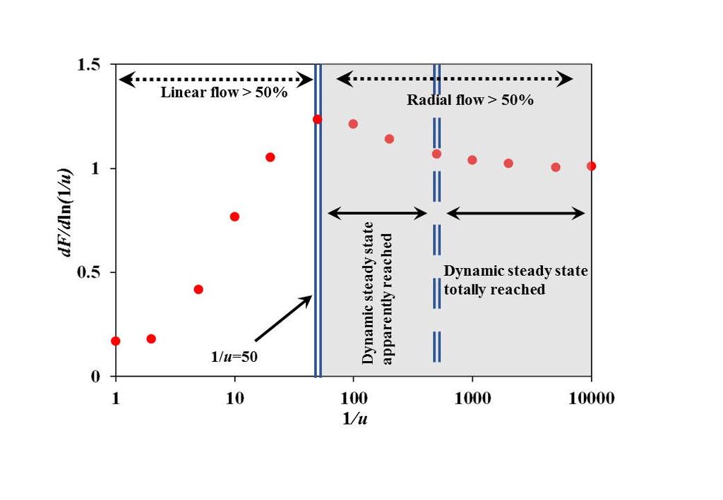
48 Figure 12