Partitioning of Unaccounted for Water for Zomba City Water Supply System in Malawi

Transcription

1 UNIVERSITY OF ZIMBABWE Partitioning of Unaccounted for Water for Zomba City Water Supply System in Malawi By Jessy Alida Chipwaila A thesis submitted in partial fulfilment of the requirements for the Master of Science Degree in Integrated Water Resources Management Department of Civil Engineering Faculty of Engineering JULY

2 Partitioning of Unaccounted for Water for Zomba City Water Supply System in Malawi A thesis submitted in partial fulfilment of the requirements for the Master of Science Degree in Integrated Water Resources Management By Jessy Alida Chipwaila Supervisor Eng. Z. Hoko JULY

3 DECLARATION I, Jessy Alida Chipwaila, do hereby declare to the Senate of the University of Zimbabwe that this product is of my own investigation except where acknowledged. This work has not been presented previously for any degree or similar award to this university or any other university. Signed.. Date.. Jessy Alida Chipwaila i

4 ABSTRACT Urban water supply utilities in developing countries are faced with challenges of low service coverage and high unaccounted for water (UFW). UFW reduces the water available to customers, and results in loss of revenue for the water utility. In Southern Africa, UFW ranges from 11% to 60% and in Malawi it is between 28% and 48%. Zomba has UFW of 30%. Most studies on UFW have not focussed on its partitioning into real and apparent loss components. Crude UFW does not allow the water utility to identify appropriate priority areas and actions for UFW reduction. It is against this background that a study was carried out on the Zomba City water supply system to partition UFW. The water supply system is owned and operated by Southern Region Water Board (SRWB). The study analysed UFW, partitioned it into its components and assessed major factors affecting the components. Four water supply zones (Airwing, Malonje, Sadzi and Mtiya) were selected based on their unique characteristics. Historical data on water production and consumption were used to assess overall UFW. Bulk meter readings for each zone were taken for three months alongside the corresponding consumptions. Flow and pressure loggers were installed to obtain Minimum Night Flows (MNF) and assess pressures respectively. Water balances were carried out. Meter inaccuracy tests were also carried out to assess the impact of meter errors on apparent losses. Records of pipe bursts, faulty meters and queries on high bills were also used in the study. The average UFW from 1999 to 2008 was estimated to be 27.5% of which real losses represented 71% while apparent losses were 29%. The average UFW for the four study zones was 13% for Airwing, 62% for Malonje, 51% for Sadzi and 6% for Mtiya. Real losses in Airwing estimated at 73% of UFW, Malonje had 75%, Sadzi had 40% and Mtiya had 23% as real losses. The remaining percentages represented apparent losses for each study site. It was also established that real losses in Airwing were due to pipe bursts mainly as a result of pipe age while in Malonje and Sadzi; the real losses were affected by bursts due to pipe age and high pressures. It was found out that more than 58% of the pipe network in the whole distribution system was over 60 years old. Malonje and Sadzi areas had operational pressures above 50 m and experienced frequent pipe bursts. It was also found out that 53% of customer meters tested were over 5 years old. Meter inaccuracy tests also showed that all the meters under-registered and that 46% of the meter errors were above the allowable tolerance of -5% at low flow rates and -2% at high flow rates. It was concluded that the average unaccounted for water was above the 20% recommended for Southern African urban water supplies. Partitioning of UFW showed that different areas had different levels of real and apparent losses and gave a hint on UFW components hence is an important tool towards proper planning of priority areas in UFW control strategies. Real losses in Airwing were affected by distribution network age, while in Malonje this was affected by pressure and distribution network age. Sadzi had a high level of apparent losses as the number of connections in the zone was very high. It is recommended that routine water audits be done for the other remaining areas to come up with a comprehensive UFW control strategy. It is also recommended that feasibility of pressure management for UFW reduction be investigated in Malonje area. Distribution network replacement is recommended in Airwing. UFW control strategy for Sadzi should focus more on reducing the high levels of apparent losses. Jessy Alida Chipwaila ii

5 DEDICATION To my beloved parents: Beatwel and Margaret Chipwaila You suffered for my JOY and I know you are proud of me! Jessy Alida Chipwaila iii

6 ACKNOWLEDGEMENTS My sincere thanks giving goes first to The Almighty God for the gift of life and education opportunity, and for always directing my paths. I also glorify God for giving me courage to take up this programme-it was not easy to make the decision when all the forces were on me! Great honour should go to the WaterNet for the full sponsorship of this IWRM programme. I would like to appreciate the work of my principal supervisor Eng. Z. Hoko. Your guidance and criticism are not taken for granted. Special thanks for your coming to Malawi during my time of research data collection-it shaped my thinking approach. I would like to thank Mr. Cosmo Ngongondo of UNIMA for his supervision. May I also extend my appreciation to the lecturers at University of Zimbabwe and all other lecturers who participated in this programme for shaping me to be a very good water manager. Many thanks should go to the Management of Southern Region Water Board for first accepting me to do the study in their Zomba City supply area and secondly for the support rendered during research period. Specifically I would like to thank the Operations Manager Mr. E. Mbesa. Many thanks should go to the Zomba Scheme Manager Mr. A. Kacheyo for the great role he played during my data collection period; his guidance, encouragement and valuable inputs are not taken for granted. I would also like to thank SSI consultants working with SRWB, for assisting me with the distribution drawings and a GPS. Many thanks should also go to Lilongwe Water Board for the data loggers. I would like also to thank Mr. M. Chiipanthenga of Blantyre Water Board for his guidance during my research. Great appreciation also goes to Mr. M. Muchotse of Mota Engil and Mr. W. Mwalughali of Anderson Engineering for their assistance during data collection. Very special thanks should go to my family: parents, sisters (Edna, Monica, Alice, Loyce, Ancity and Veronica) and brother (Austin) for tirelessly being with me in everything during my entire study and research period. Special honour has to go to Mr. and Mrs. Unyolo and Ms B. Sambakunsi for all the support they gave me during my data collection. Many thanks go to IWRM 2008 class for being a very great class. To my special buddies: Elina Lusuva, Andrea Vushe and Richman Kalua - you have been the source of my inspiration and I owe you a great debt of honour. The list is long God bless you all!! Jessy Alida Chipwaila iv

7 LIST OF ACRONYMS AWWA BL DMA ESIA GI ICTR ILI ISO IWA IWRM MBF MNF MWD NNF NRW NSO NWDP OFWAT PI PVC SADC SANFLOW SIDA SRWB TIRL TWL UARL UFW UNEP UNIMA WDM ZDA ZMA American Water Works Association Background Leakage District Metered Area Environmental and Socio Impact Assessment Galvanised Iron Institute of Corporate Training and Research Infrastructure Leakage Index International Organization for Standardization International Water Association Integrated Water Resources Management Mains Break Frequency Minimum Night Flow Ministry of Water Development Net Night Flow Non Revenue Water National Statistical Office National water Development Programme Office of Water Services Performance Indicator Poly Vinyl Chloride Southern Africa Development Community South African Night Flow Analysis Swedish International Development Agency Southern Region Water Board Technical Indicator for Real Losses Top Water Level Unavoidable Annual Real Loses Unaccounted For Water United Nations Environmental Programme University of Malawi Water Demand Management Zomba District Assembly Zone Metered Area Jessy Alida Chipwaila v

8 CONTENTS DECLARATION... i ABSTRACT... ii DEDICATION...iii ACKNOWLEDGEMENTS... iv LIST OF ACRONYMS... v LIST OF TABLES... ix LIST OF FIGURES... x 1.0 INTRODUCTION Background Problem statement Justification Objectives Main objective Specific Objectives LITERATURE REVIEW Introduction Unaccounted for Water Components of Unaccounted for Water Apparent losses Assessment of Apparent Losses Real Losses Assessment of Real Losses Ways to minimize Real losses Performance Indicators STUDY AREA Location Topography, Geology and Climate Vegetation and Environment Jessy Alida Chipwaila vi

9 3.4 Land Use Socio-economics Population Size and Growth Water resources Water Supply Urban and peri-urban areas in Malawi Zomba City Specific Study Areas MATERIALS AND METHODS Study Design Data Collection Trends of unaccounted for water UFW for specific study areas Partitioning of UFW System characteristics influencing UFW Data analysis Trends of unaccounted for water UFW for specific study areas Partitioning of UFW RESULTS AND DISCUSSION Trend of unaccounted for water for Zomba City Unaccounted for Water and its partitioning for the specific study areas Unaccounted for water for study areas Partitioning of unaccounted for water System characteristics influencing UFW Pressure and Real Losses Age of distribution mains and Real losses Meter inaccuracies and Apparent Losses Tank overflows Relationships between system characteristics and unaccounted for water CONCLUSIONS AND RECOMMENDATIONS Jessy Alida Chipwaila vii

10 6.1 Conclusions Recommendations REFERENCES APPENDICES Appendix I: Unaccounted for Water for Zomba City from 1999 to Appendix II: Tank meter readings and monthly consumption Appendix III: Data logging points attributes Appendix IV-a: Airwing Tank Flow Logging Results Appendix IV-b: Malonje Tank Flow Logging Results Appendix IV-c: Sadzi Tank Flow Logging Results Appendix IV-d: Mtiya Tank Flow Logging Results Appendix V-a: Airwing Zone Pressure Logging Results Appendix V-b: Malonje Zone Pressure Logging Results Appendix Vc: Sadzi Zone Pressure Logging Results Appendix V-d: Mtiya Zone Pressure Logging Results Appendix VI-a: Airwing MNF Analysis using SANFLOW Model Appendix VI-b: Malonje MNF Analysis Appendix VI-c: Sadzi MNF Analysis Appendix VII: Bucket tests results and pipe network installed in Appendix VIII: Summary of pipe burst records for 2007 and Appendix IX: Some high bills between 2007 and Appendix X-a: Airwing Meter Inaccuracy Tests Appendix X-b: Malonje Meter Inaccuracy Tests Appendix X-c: Sadzi Meter Inaccuracy Tests Appendix X-d: Mtiya Meter Inaccuracy Tests Appendix XI: Map of Zomba Appendix XII Zomba City water supply pressure zones Appendix XIII Research Pictures Jessy Alida Chipwaila viii

11 LIST OF TABLES Table 2-1: The IWA best practice standard water balance... 7 Table 2-2: Composition of UFW... 9 Table 3-1: Details of Study Areas Table 4-1: Data collection: Monitoring and Frequency Table 4-2: Infrastructure variables used in SANFLOW Model Table 4-3: Leakage Parameters Used in SANFLOW Model Table 5-1: Yearly unaccounted for water for Zomba City water supply system Table 5-2: Consumption billed for the four study areas Table 5-3: Water supply to the four study areas Table 5-4: Average UFW for the four supply areas Table 5-5: Unaccounted for water for February Table 5-6: MNF for the period 27 March to 9 April Table 5-7: Real losses obtained from MNF analysis Table 5-8: Partitioning of UFW Table 5-9: ILI for study areas Table 5-10: Zomba City UFW partitioning based on meter errors Table 5-11: Distribution losses for Zomba based on results from study areas Table 5-12: Zomba City UFW partitioning based on distribution losses Table 5-13: Revenue loss due to UFW in Zomba City Table 5-14: Maximum Night Pressures for logged points in the study areas Table 5-15: Mains age and unaccounted for water Table 5-16: Distribution of meters tested in study areas Table 5-17: Results of Meter Inaccuracy Tests Table 5-18: Key for summary of factors affecting UFW Table 5-19: Parameters for meter age and apparent losses Table 5-20: Error assessment for apparent loss due to meter age Table 5-21: Parameters for number of connection and apparent losses Table 5-22: Error assessment for apparent loss based on number of connections Jessy Alida Chipwaila ix

12 LIST OF FIGURES Fig. 2-1: Components of a proactive apparent loss management program Fig. 2-2: Customer meter error curve Fig. 2-3: Components of real losses Fig. 2-4: Components of a proactive real loss management program Fig. 3-1: Urban water supply coverage in Malawi Fig. 3-2: Schematic of Zomba City water supply showing specific study areas Fig. 3-3: Zomba City water distribution system showing study areas Fig. 5-1: Total water produced, billed and UFW for Zomba City from 1999 to Fig. 5-2: Airwing Tank outflow pattern Fig. 5-3: Malonje Tank outflow pattern Fig. 5-4: Sadzi Tank outflow pattern Fig. 5-5: Real losses and Pressure Fig. 5-6: Airwing outflow and pressure patterns Fig. 5-7: Malonje outflow and pressure patterns Fig. 5-8: Mtiya pressure pattern Fig. 5-9: Sadzi outflow and pressure patterns Fig. 5-10: Meter curves for selected meters Fig. 5-11: Age of meters and error unacceptability Fig. 5-12: Influence of system characteristics on UFW Fig. 5-13: Relationship between apparent losses and meter age Fig. 5-14: Relationship between apparent losses and number of connections Fig. 5-15: Service quality in terms of pressure and filling times Jessy Alida Chipwaila x

13 CHAPTER ONE 1.0 INTRODUCTION 1.1 Background In the year 2000, about 1.16 billion people had no access to improved water sources and double as much (2.36 billion people) had no access to adequate sanitation worldwide (UNDP, 2003). According to UNDP (2003), Sub-Saharan Africa accounts for about 23% of the global total population without access to improved water sources. The Millennium Development Goals (MDGs) recognize that access to safe water is crucial for survival and aim to halve the proportion of people without sustainable access to safe drinking water by 2015 (UNDP, 2003). According to Baietti et al. (2006), the challenge to provide adequate safe drinking water and improved sanitation require well performing water utilities. For many years more than 90% of urban water supply and sanitation services in developing countries have been provided by state-owned, monolithic water organizations also known as public water utilities (Ndokosho et al., 2007). As part of a general move to market oriented systems in the 1980s and 1990s, a new paradigm emerged to transform utilities into more modern service delivery organizations that emphasize operational and financial sustainability (Baietti et al., 2006). In many developing countries public water service providers have failed to provide consumers with adequate water supply and sanitation services (Baietti et al., 2006). Apart from the problems of service coverage of less than 60%, other problems that are faced by water utilities in these developing countries include overstaffing and high unaccounted for water (UFW), which often averages between 40%-60% (Baietti et al., 2006; Schwartz, 2008). According to Balkaran and Wyke (2002), UFW is between 15% and 30% in the developed world but elsewhere it is more likely to be in the 30% to 60% range. Moreover, the service providers in developing countries are often confronted with financial problems due to a combination of low tariffs, poor consumer records and inefficient billing and collection practices (Schwartz and van Dijk, 2007). As a result, the quality of water services that is actually delivered to the consumer, if they are connected at all, is low (Schwartz, 2006). The public water utilities, which are likely to remain responsible for service provision for many years to come do not have satisfactory performance and provide inadequate services to their customers (Schwartz, 2006). Unaccounted for water (UFW) often constitutes a major problem in water supply, representing considerable loss in revenues, creating excessive production and reducing the available water to customers (SIDA, 2000). According to Schwartz (2008), high levels of unaccounted for water indicate inefficiency on the side of a water utility as UFW is a crude measure of the utility s performance. According to Yepes and Dianderas (1996), the level of UFW is considered a good proxy for the overall efficiency of operations of a water utility. Tynan and Kingdom (2002) indicate that a crude measure of asset maintenance is unaccounted for water. The measure captures not only physical losses but also commercial losses, due to inefficient billing or illegal connections. Thus according to Tynan and Kingdom (2002), high levels of unaccounted for water indicate poor system management and poor commercial practices as well as inadequate pipeline maintenance. This agrees with assertions by Yepes and Dianderas (1996) and Schwartz Jessy Alida Chipwaila 1

14 (2008). The World Bank recommends a UFW of 23% (Tynan and Kingdom, 2002) in developing countries, while 20% was set for well performing urban water utilities in Southern African region (Gumbo, 2004). With the increasing international trend towards sustainability, economic efficiency and protection of the environment (Savenije & Van der Zaag, 2002), the problem of losses from water supply systems is of major interest world-wide (Lambert and Hirner, 2000). Both the technical and the financial aspects are receiving increasing attention, especially during water shortage or periods of rapid development. One of the Integrated Water Resources Management (IWRM) three key policy principles is efficiency which states that water is a scarce resource hence should be used efficiently. Therefore assessment and control of UFW is a major component towards achieving efficient use of water. According to Savenije & Van der Zaag (2003), UFW control ensures sustainability of infrastructure (sustainable development), postponement of investment and availability of water to other new customers; this supports the equity principle. UFW assessment and control aims to achieve desirable consumption patterns, both in terms of distribution among sectors and quantities consumed, coupled with an increased reliability of supply (Savenije & Van der Zaag, 2003). This agrees with Lambert and Hirner (2000) who indicate that water loss control is a key to improved water demand management. In most of the water supply systems in Southern Africa, reliable estimates of water loss components are not available (Farley, 2001). Since UFW occurs as both real and apparent losses; reporting a crude figure of UFW makes it difficult to establish areas of priority when it comes to UFW management. Southern Region Water Board presents unaccounted for water as a crude figure (SRWB, 2008a). The utility does not have the quantification of real and apparent losses. It is against this background that the study was carried out to partition UFW into real and apparent loss components in Zomba City water supply system. The water supply system is owned and operated by the SRWB. Urban and peri-urban water services in Malawi are provided by water boards. The Regional Water Boards inherited very old and inefficient water supply facilities from the District Water Supply Fund which was formerly responsible for supplying water in small urban areas in Malawi (Mulwafu et al., 2002). In Zomba City, the old facilities are responsible for high losses of water through leakage. The poor conditions of the old pipelines result in frequent pipe bursts (SRWB, ). There are also issues of faulty meters and problems of uneven pressure in the water supply systems that can cause pipe bursts. Management of unaccounted for water in the distribution system will improve service delivery, as some of the areas in the city are currently experiencing water shortages (SRWB, ). The study was carried out in the four specific zones which were Airwing, Malonje, Mtiya and Sadzi. All these zones have individual water connections but very few connections in Mtiya and Sadzi are communal water points (CWPs). The entire Zomba City has a total of 79 CWPs (SRWB, ). Approximately 70% of the study areas are traditional and high density areas whereby those connected to SRWB water supply have single taps. The other percentage has multiple in-house taps. Malonje is reported to have high level of Jessy Alida Chipwaila 2

15 reported problems which include pipe bursts and water shortages (SRWB, ) and 40% of the population relies on boreholes, indicating low coverage and water supply inefficiencies by SRWB. From the socio-economic survey done by SRWB () it was reviewed that Malonje, Mtiya and Sadzi had low coverage of piped water supply of 65%. 1.2 Problem statement Many water utilities have managed to quantify their total unaccounted for water (UFW). Urban water supply systems in Southern Africa have UFW ranging from 11 to 60% and in Malawi, the unaccounted for water ranges between 28% and 48% (World Bank, 2007). Unaccounted for water for Zomba City is at 30% (SRWB, 2008a). In most of the water supply systems in Southern Africa, reliable estimates of water loss components are not available (Farley, 2001). A crude figure of UFW which is reported by many water utilities does not give the water utility clues to prioritise and schedule on the operations and management of the system (Kingdom et al., 2006). It is for this reason that a study was carried out in Zomba City water supply area, to partition unaccounted for water, into real and apparent losses; and to establish the major contributing factors to the current water losses in the system. 1.3 Justification The UFW for Zomba city is currently high at around 30% (SRWB, ), and the SRWB aim to reduce this to 20% by Almost 58% of the distribution mains are old network and the poor conditions of the old pipelines result in frequent pipe bursts as reported by SRWB (). Management of unaccounted for water in the distribution system will improve on water demand management, as some of the areas in the city such as some parts of Malonje and Mtiya are currently experiencing water shortages (SRWB, ). Identification of priority areas and effectiveness on the UFW reduction can be achieved if water audits and UFW partitioning are carried out. According to Liemberger (2002), real and apparent losses have to be quantified. No proper unaccounted for water reduction strategy can be planned without the quantification of physical and apparent (commercial) losses (Kingdom et al., 2006). When the magnitude of all components is known it is possible to forecast potential savings (real losses) and potential revenue increase (apparent losses), develop real and apparent loss reduction strategies and set realistic targets (Liemberger, 2002). Thus breaking down unaccounted for water may assist the water utility to improve knowledge and documentation of the distribution system including problem and risk areas. The breakdown and hence the water audit also becomes a valuable tool to manage resources, by getting a better understanding of what is happening to the water after it leaves the treatment plant. Thornton (2002) indicates that water loss reduction programmes lead to reduced water losses, financial improvement, increased knowledge of the distribution system, more efficient use of existing supplies, safeguarding public health and property, improved public relations, reduced legal liability, and reduced disruption of water supply to customers. Jessy Alida Chipwaila 3

16 1.4 Objectives Main objective The main objective of the study was to assess and partition unaccounted for water into real and apparent losses for Zomba City water supply system and to analyse system characteristics in order to predict UFW trends for better operation and management of the water system Specific Objectives The specific objectives of the study were: To establish the trends of unaccounted for water for Zomba city from 1999 to To establish unaccounted for water in selected parts of the Zomba City water supply area, partition it into real and apparent losses and further assess the revenue loss due to the unaccounted for water in the system To analyse system characteristics such as pressure, pipe age, bursts, meter inaccuracy, tank overflows; and identify the most significant ones with respect to UFW in the area. To develop relationships that will describe and predict the unaccounted for water with respect to system characteristics for better operation and management of the water system. Jessy Alida Chipwaila 4

17 CHAPTER TWO 2.0 LITERATURE REVIEW 2.1 Introduction Most of the water on the earth, some 97%, is contained in the world's oceans and is therefore not for essential agriculture, drinking, or most industrial uses (Butts, 1997). Moreover only 0.36% of the world's water in rivers, lakes, and swamps is sufficiently accessible to be considered a renewable fresh water resource (Butts, 1997). The supplies of useful fresh water are finite, and most of the forms in which it is used have no substitute. In 2000 a global population of 1.16 billion people lacked adequate potable water supply (UNDP, 2003). Water constitutes a worldwide challenge for the 21 st century, both in terms of the management of available water resources and the provision of access to drinking water and sanitation for the world s population (UNDP, 2003; SADC, 2005). Projections of population, water demand, and water development indicate that by 2025 some countries in the Southern African region will experience water quality and quantity problems in the dry season and others will experience water stress (SADC, 2005). Malawi and South Africa will experience absolute scarcity where the fresh water resources distribution will be less than 1000 l/capita/yr (UNEP, 1999; SADC, 2005). It can be deduced that water shortage and scarcity has now become a global concern and poor management of water resources can exacerbates its unavailability. An essential component of water demand for public water supply may be the losses in transport, treatment and distribution systems normally known as unaccounted for water (ICTR, 2005). ICTR (2005) suggests that UFW may reach levels of 60% in old and deteriorated systems. According to Balkaran and Wyke (2002) unaccounted for water (UFW) also known as water losses, is between 15% and 30% in the developed world but elsewhere it is more likely to be in the range of 30% to 60%. UFW in the range of 40% to 60 % is far often the case in urban distribution systems in the developing world (SIDA, 2000; Baietti et al., 2006; Schwartz, 2008). In Malawi unaccounted for water ranges between 28% and 48% (World Bank, 2007). UFW in most developing urban water utilities is very high compared to the international standards set. Van der Zaag (2003) states that the normal percentages for unaccounted for water in the system are from 15% to 25%, including a 5% loss in the treatment plants and SIDA (2000) reports that UFW in the range of up to 15% to 20% of the produced quantity is often a realistic and sustainable level for developing countries. Public water utilities have a duty to ensure UFW control in order to achieve sustainable and efficient water supply systems. According to SIDA (2000) unaccounted for water through leaking pipes, overflows from tanks, illegal connections, metering errors and non-metered uses in the water production, poor plumbing and other faults in the system very often constitutes a major problem in water supply resulting in considerable loss in revenues and excessive production. SIDA (2000) states that comprehensive water loss control programmes are often priority issues in urban water supply rehabilitation and improvement projects. Contrary to this, Schwartz (2008) indicated that operation and maintenance in water supply has a low, and usually an inferior profile as compared to new construction and system extension. According to Schwartz (2008), while water utilities get funding for new construction; little money and Jessy Alida Chipwaila 5

18 attention is given for operations and asset maintenance. The challenge is that unaccounted for water may exceed one quarter of the water put into supply, and according to Balkaran and Wyke (2002) this can represent a substantial financial loss to any water undertaking. It is suggested therefore that water demand management (WDM) with improvements to the existing water supply systems should be pursued before construction of new and costly systems are undertaken. UFW assessment and control in a water utility is important as there are considerable reduction in water shortages, improvement in revenue and postponement of major infrastructure investment on water supply system. Thus as one of the major WDM tools UFW control needs to be pursued. 2.2 Unaccounted for Water Unaccounted for water is the difference between the amount of water produced, or purchased, and the amount of water sold to all customers (Johnson, 1996). UFW includes underground leakage; unauthorized use; unavoidable leakage, inaccurate master, industrial, commercial and domestic meters and unusual causes (Johnson, 1996). According to Johnson (1996), unusual causes include one of the following: recirculating water, that is, water pumped into a pressure zone with an open valve which allows the water to recirculate without being consumed; not accounting for treatment plant use; estimated pumping rate due to inaccurate or non-existent meters; leakage in reservoirs, ground storage tanks or elevated storage tanks; and unintentional inter-system connections where water passing through is unrecorded or there are emergency connections to other distribution systems. There are different definitions and words to describe unaccounted for water which mostly confuse the readers. According to Thornton (2002) the problems of water and revenue losses are divided into three. There are technical problems where not all water supplied by a water utility reaches the customer; financial problems where not all of the water that reaches the end user is properly measured or paid for and terminological problems where standardized definitions of water and revenue loses are lacking (Thornton, 2002). Johnson s definition of unaccounted for water did not break it down into its categories. Based on the International Water Association (IWA), there are two major categories under which all types of supplier loss occurrences fall (Lambert and Hirner, 2000). These are real and apparent losses. Real losses are physical escape of water from the distribution system, and include leakage and overflows prior to the point of end use (Lambert and Hirner, 2000). This can be synonymous with technical problems of water and revenue losses as presented by Thornton (2002). Apparent losses are essentially losses consisting of customer use which is not recorded due to metering error, incorrect assumptions of unmeasured consumption and water theft (Fanner, 2004) and this definition is similar to the financial problems of water and revenue losses as described by Thornton (2002). Unaccounted for water should be broken down into its components to ease their assessment and reduction. According to KWA (2002) a high percentage of unaccounted for water in a public water utility may arise when the utility has: Inaccurately estimated the amount of water pumped or purchased due to no metering of all water at the intake source or by using raw water or finished water meters that are inaccurate or improperly installed; Jessy Alida Chipwaila 6

19 Inaccurate customer meters; Bookkeeping errors; Non-metered uses such as water used in the treatment process, city buildings, churches, watering a golf course; Water leaks. Table 2-1 gives the IWA standard water balance which just like in financial cash balance analysis and auditing, is where the amount of water put into distribution is compared with the sum of the components of water consumed or used (Farley, 2001). Further to this table are the steps used to calculate the components of the water balance and are presented after Table 2-1. Table 2-1: The IWA best practice standard water balance Own Sources Water Imported Corrected System Input Volume (Adopted from Fanner, 2004) Water Export Water Supply Authorized Consumption Water Losses (UFW) Billed Water Billed Exported Billed Metered Authorized Consumption Consumption Billed Un-metered Consumption Unbilled Unbilled Metered Authorized Consumption Consumption Unbilled Unmetered Consumption Unauthorized Consumption Apparent Losses Real Losses Customer Metering Inaccuracies and Data Handling Errors Leakage on Transmission and/or Distribution Mains Leakage and Overflows at Utility s Storage Tanks Leakage on Service Connections up to point of Customer metering Revenue Water Non- Revenue Water (NRW) Jessy Alida Chipwaila 7

20 Steps for calculating non-revenue water and water losses (adopted from Lambert and Hirner, 2000). The following steps are used to obtain components of the water balance, which at the end enable the water utility to calculate its water losses and non-revenue water. The steps refer to Table 2-1 above which has seven (7) columns. Step 1: Define sources of water and enter in Col. 1. Step 2: Define corrected System Input Volume as sum of Col 1 and enter in Col. 2. Col. 3 represents total water diverted by the water utility and this can either be exported to other water utility or can be supplied to the utility s customers. Step 3: Define Billed Metered Consumption, Billed Unmetered Consumption and Billed water exported in Col. 6; enter total in Billed Authorised Consumption (Col. 5) and Revenue Water (Col. 7). Step 4: Calculate the volume of Non-Revenue Water (Col. 7) as corrected System Input Volume (Col. 2) minus Revenue Water (Col. 7). Step 5: Define Unbilled Metered Consumption and Unbilled Unmetered Consumption in Col. 6; transfer total to Unbilled Authorised Consumption in Col. 5. Step 6: Add volumes of Billed Authorised Consumption and Unbilled Authorised Consumption in Col. C; enter sum as Authorised Consumption (top of Col. 4). Step 7: Calculate Water Losses (Col. 4) as the difference between corrected System Input Volume (Col. 2) and Authorised Consumption (Col. 4). Step 8: Assess components of Unauthorised Consumption and Metering Inaccuracies and data handling errors (Col. 6) by best means available, add these and enter sum in Apparent Losses (Col. 5). Step 9: Calculate Real Losses (Col. 5) as Water Losses (Col. 4) minus Apparent Losses (Col. 5). Step 10: Assess components of real losses (Col. 6) by best means available (night flow analysis, burst frequency/flow rate/duration calculations, modelling etc), add these and cross-check with volume of Real Losses in Col. 5 which was derived from Step 9. From Table 2-1, the difference between non-revenue water and water losses can be seen in that non-revenue water represents unbilled authorized consumption, apparent losses and real losses while water loss or unaccounted for water represents apparent and real losses. The UFW can be considered as a total volume for the whole system, or for partial Jessy Alida Chipwaila 8

21 systems such as raw water mains, transmission or distribution (Lambert and Hirner, 2000). And where UFW analysis is carried out for the distribution network or zone, it is referred to distribution losses (Lambert and Hirner, 2000). In each case the components of the calculation would be adjusted accordingly. There are many causes of UFW in the water supply system and each cause may contribute differently to UFW. For successful control of UFW, all the technical, financial and terminological aspects of UFW need to be understood by the water utility. This includes assessment of UFW using the IWA standard water balance. 2.3 Components of Unaccounted for Water UFW is broken down into two main components which are real (physical) losses and apparent (commercial) losses (Yepes and Dianderas, 1996). A few methodologies have been developed to assess the unaccounted for water in water distribution systems, however most of them just concentrate on the real losses concept, and have no emphasis on the apparent losses, which is so important in most undeveloped and developing countries (Tabesh and Asadiani Yekta, 2005). In most cases, unaccounted for water is presented as a crude figure that is, it is not broken down into its components. For instance, for well performing water utilities, the World Bank set 23% as unaccounted for water in developing countries (Tynan and Kingdom, 2002). Baietti et al., (2006) listed levels of unaccounted for water and circumstances which give rise to such losses without stating how much constitutes real or apparent loss components. This indicates that most of the studies done do not further on to partition UFW. Contrary to this, some water utilities like those in South Africa have calculated components of non-revenue water, apparent losses and real losses using the standard annual water balance and have further developed software tools to enable reduction of UFW (Mckenzie et al., 2002b). Unaccounted for water is a problem for all water utilities (Balkaran and Wyke, 2002) and the need to know the causes and quantities of the various components of UFW is obvious and has to be emphasized (Kingdom et al., 2006). Table 2-2 presents the composition of UFW for some selected cities as reported by Yepes and Dianderas (1996). Table 2-2: Composition of UFW Country/City Year Physical (%) Commercial (%) Total (%) Singapore Spain, Barcelona Colombia, Bogota Costa Rica, San Jose (Source: Yepes and Dianderas, 1996) The table suggests that the issue of UFW partitioning, although has been taken up by few water utilities, is not new; for example, the table shows that Singapore partitioned UFW in Therefore UFW partitioning should not be taken as a new subject. Yepes and Dianderas (1996) presented unaccounted for water in terms of its two components. From Table 2-2, it can be seen that each of the two components contribute significantly to UFW, contrary to the common assumption that real losses are always greater than Jessy Alida Chipwaila 9

22 apparent losses. Farley (2001) indicates that the studies of Vietnamese water companies established that around two-thirds of losses are due to non-physical losses (apparent losses) and one-third are due to physical losses. Real losses in the system may dominate if that system has old distribution pipelines which can no longer withstand high pressures and experience a lot of bursts and leaks. Unavailability of customer cadastre, reluctance on meter repairs and poor accountability to customers may lead to high levels of apparent losses. Thus presenting unaccounted for water as a crude figure may not enable the water utility visualise how each component is contributing to total UFW and hence may not be able to narrow down to areas of priority during unaccounted for water control programmes. 2.4 Apparent losses Apparent losses (AL) consist of unauthorized consumption (theft or illegal use), and all types of inaccuracies associated with production metering and customer metering (Lambert and Hirner, 2000; Tabesh and Asadiani Yekta, 2005). Apparent water losses can be perceived as occurring in three primary ways (Lambert and Hirner, 2000). According to Lambert and Hirner (2000) these losses occur as a result of errors in water flow measurement, errors in water accounting and unauthorised usage or theft. They are related to management losses resulting in a shortfall of revenue for water supplied (Farley, 2001). Because this water was available for sale, these losses are incurred at retail rate (Tabesh and Asadiani Yekta, 2005). Under-registration of production meters and over-registration of customer meters lead to under-estimation of real losses; and over-registration of production meters and under-registration of customer meters, lead to over-estimation of real losses (Lambert and Hirner, 2000). Hence an inappropriate assessment of apparent losses often results in real losses being overstated in the water audit, potentially misguiding water loss optimisation planning by placing inordinate emphasis on leakage while potential revenue recovery goes unattended (Thornton, 2002). This reveals that assessment of apparent losses has a direct impact of real losses and therefore it is important to pay attention to both components of unaccounted for water. Further to the IWA standard water balance in Table 2-1, apparent losses are broken down into four component errors (IWA, 2008). There are losses due to under-metering which refers to the errors generated by the water meters themselves or by the management of the water meters where the meter does not completely register the volume passing through them (Rizzo et al., 2004). For unmetered customers, estimation of unmetered consumption also generates errors. This is a very important component for systems that are not fully metered (Rizzo et al., 2004; IWA, 2008). Unauthorised consumption is another component of apparent losses which refers to unregistered water connection and any kind of frauds or malpractice (Tabesh and Asadiani Yekta, 2005). According to Rizzo et al. (2004), unauthorised consumption comprises theft and any form of illegal consumption. The fourth error component of apparent losses is linked to data acquisition system which, according to IWA (2008), refers to the errors that may be generated at the various stages of the data acquisition process such as data capture (meter readings and computer system data entry), transmittal, processing, manipulation etc. According to Rizzo et al., (2004) data acquisition errors are data transfer errors between meter and billing system and data analysis between archived. Assessment of apparent losses is Jessy Alida Chipwaila 10

23 therefore supposed to target these four components. Consequent to the four categories of apparent losses, there are four categories of actions, as presented in Fig. 2-1 that can be implemented to get the apparent losses under control (Thornton, 2005). Customer accountability data integrity controls Policy enforcement control Current level of AL Economic level of AL Unavoidable AL Customer meter management Data handling and analysis control Fig. 2-1: Components of a proactive apparent loss management program (Adopted from Rizzo et al., 2004) The level of apparent loss may increase or decrease depending on the level of control of each category of loss. One of the major characteristic of the apparent losses is that they can be positive or negative (IWA, 2008). For instance a water meter may over-register in some specific conditions; and a non-metered consumption can be overestimated (IWA, 2008). Working on the four reduction strategies presented in Fig. 2-1 is a key to reduced apparent losses Assessment of Apparent Losses There are various factors affecting apparent losses as discussed in the previous section and these can be assessed in different ways. The proceeding discussion looks at ways of determining their quantities which can later be used in the water balance analysis. Under-registration by customers meters This concept reflects the fact that the water metering devices do not actually display an exact readout of the water volume that passes through them (Sánchez, 2007). This is influenced by several factors. Customer meters tend to under-register as a result of meter aging, inappropriate meter installation, inappropriate sizing and impacts of customers inhouse installation. Meter mismanagement also result in meter under-registering or errors. This includes errors in meter reading, invented meter reading and when the meter is out of operation (IWA, 2008). Jessy Alida Chipwaila 11

24 Meters that under-register can be estimated from a sample survey (Sánchez, 2007). Accurate C or D class meters, may be temporarily installed in line with the customer s meter, as check meters to compare the volume flows. A meter test bench which has an inbuilt calibrated meter can also be used if available (IWA, 2008). Other organizations have used a 200 l calibrated drum and checked the accuracy of the meter under test by filling the drum to a mark of 200 l, and reading the volume that has passed through the meter. The volume which is lost due to under-registration in the surveyed area is calculated and extrapolated. According to Sánchez (2007) calculation of metering errors is solely executed in accordance to the age of the metering device. Inaccuracy is determined for each metering device in a % over its readout, based on the age of the device counted since the date of its installation. The error percentage, which is then multiplied by the recorded amount (metered billed and/or metered unbilled in the period of analysis), is assigned to the meters per linear distribution (Sánchez, 2007). Meter Error Curve Meter inaccuracy depends on the flow rate at which the meter is being used (IWA, 2008). Studies have reviewed that residential consumption typically occurs at 5, 15, and 80 percent for low, medium, and high flows, respectively. A study carried out in Detroit Water and Sewage Department (DWSD, 2004) concluded that 15- to 20-year-old allbrass meters (no longer manufactured) have an overall accuracy of 98.5 to 99% while 15- year-old meters with plastic drives have tested out at 95% accuracy. In another study, in Australia, DWSD (2004) indicated that 6% of the water delivered to 11,000 residential properties was not measured due to inaccuracy in the flow meters, but nothing is mentioned in regarding the age and calibration of meters. The meter has to be tested at different flow rates to give different errors from which a meter error curve is established (Sánchez, 2007; IWA, 2008). For better use of the results from the meter survey, the water utility has to know its customers and their consumption patterns, that is, the category in which the customer falls; how much the customer uses and at what flow rates. When the meters have been tested, the water utility can have a picture on what kind of the meter a customer requires so that the utility does not lose a lot of revenue through meter under registering or errors. Fig. 2-2 shows the meter error curve. The 2% and 5% values for new meters are suggested by international standard (ISO) (IWA, 2008). The curve of the meter should always be located inside what is called the tunnel (IWA, 2008). This indicates a normal operating meter which is under-registering to acceptable levels. Fig. 2-2 shows that even with a new meter, the error (under-metering) may be very high when the consumption flow rate is small. The error is 100% under the start-up flow rate. The meter should not be used for flow rates lower than the minimum flow rate (IWA, 2008). But the customer s consumption is what it is: this is the reason why, even with new meters, there is always a volume of water consumed that is not metered that is apparent loss. Jessy Alida Chipwaila 12

25 Error 5% 0% ±5% ±2% -5% -10% -15% -20% -25% Startup Minimum Transitional Flow rate l/hr Fig. 2-2: Customer meter error curve (Adopted from Actaris Meter Systems, 2004) Stopped or broken meters Stopped or broken meters record zero flow when the customer is actually using the water (IWA, 2008). Average consumption on the other hand does not represent the true consumption of the customer and usually under-estimates the consumption. The number of these can be estimated from meter records or a sample survey (Farley, 2001). During meter readings, meter readers take records of all meters which are stuck and are not recording at all. Volume lost due to stuck meters can be calculated from meter records or from estimates of per capita consumption (Farley, 2001). Meter records give an average consumption of the customer based on the past consumption patterns. Unauthorised use Unauthorized use is an area often overlooked in trying to reduce unaccounted for water. Unauthorized use can consist of unmetered use by contractors; unauthorized or unmetered connections; and theft by bypassing meters. Unauthorized use, especially in older systems, can be one of the most difficult areas to eliminate in trying to reduce unaccounted for water (Johnson, 1996). As in real losses, the most important first step that must be taken with regard to apparent losses is in their quantification, or measurement. Unless some idea is known about the volume of water that is being consumed but not being paid for, little support will be provided by the organization concerned to reduce this apparent loss (Rizzo et al., 2004). It can also not be concluded that the apparent losses are low in a water utility by just Jessy Alida Chipwaila 13

26 looking at a large number of new meters installed, as meter errors are not the only factor influencing apparent losses and literature has also revealed that even a new meter underregisters to some degree; quantification is the only way to confirm that the apparent losses are indeed low. 2.5 Real Losses Real losses (RL) are physical water losses from the pressurised system, up to the point of customer metering (Farley, 2001). According to Tabesh and Asadiani Yekta (2005), real losses are categorised as water losses from reported and unreported bursts, background losses, reservoir leakage and overflow and leakage from valves and pumps. Because this water did not have the opportunity to pass through a customer s meter, Tabesh and Asadiani Yekta (2005) indicate that these losses are incurred at the production rate. Further to this, Farley (2001) argues that since real losses comprise physical water losses from the water supply system, real losses lead to reduced supply to customers. The IWA recommended definition for real losses is the annual volumes lost from transmission and distribution systems through all types of leaks, bursts and overflows on mains, service reservoirs and service connections, up to the point of customer metering (Thornton and Lambert, 2005). Leaking systems may present substantial threats to public health, because of possibilities for infiltration of contaminated groundwater under low pressure conditions in the distribution network (Tabesh and Asadiani Yekta, 2005). Leak detection programs are effective ways to minimize leakage and to fix small problems before they become major ones (Water Audit Guidance, 2008). Thus real loss control through leak management is essential not only to avail water to customers but to protect the public health as well. Fig. 2-3 presents the components of real losses. Leakage and overflows at storage Leakage on mains Current level of RL Economic level of RL Unavoidable RL Leakage on service connections Background leakages on pipes Fig. 2-3: Components of real losses (Adopted from Thornton, 2005) Jessy Alida Chipwaila 14

27 Measures to control real losses should be applied simultaneously on the four components in Fig Initial efforts can reduce real losses from current level to economic level of real losses. Further reduction of these components will reduce real losses to unavoidable real losses where further reduction will not be economical (Thornton, 2005). Fig. 2-4 provides the proactive real loss control program. Pressure Management Improved Leak repair Time Current level of RL Economic level of RL Unavoidable RL Proactive Leak Detection Infrastructure Management Fig. 2-4: Components of a proactive real loss management program (Source: Thornton, 2005) There are four major components to real loss control which aim to reduce the four real loss components presented in Fig The number of new leaks arising each year is influenced primarily by long-term infrastructure or pipeline and asset management which includes selection, installation, maintenance, renewal and replacement. Pressure Management can influence the frequency of new leaks, and the flow rates of all leaks and bursts (Lambert, 2002). The average duration of the leaks is limited by the speed and quality of repairs, that is, improved leak repair time, and the proactive leakage control strategy controls how long unreported leaks run for before they are located (Thornton, 2005). The extent to which each of these four activities is carried out will determine whether the volume of annual Real Losses increases, decreases or remains constant (Lambert, 2002). To keep real losses at minimum, that is, to squeeze the real loss box, the four measures in Fig. 2-4 have to be employed effectively Assessment of Real Losses There are various components of real losses and these can be assessed in different ways (Farley, 2001). The proceeding discussion looks at the components and ways of determining their quantities which can later be used in the water balance analysis. Reservoir Leaks Leakage from reservoirs can be measured by the reservoir drop test. The inlet and outlet valves of the reservoir are closed and the drop in water level over a period of time is Jessy Alida Chipwaila 15

28 measured. For reservoirs which have compartments, each can be monitored in turn. According to Farley (2001), drop tests are usually carried out at night to minimize disruption to the supply. Reservoir overflows Overflows from reservoirs are assessed by inspecting the float valves when the reservoir is at top water level (TWL). The volume passing for the period when the reservoir is at TWL is estimated or measured (Lambert and Hirner, 2000). Leakage from trunk mains Assessment of leakage from trunk mains can be done by inserting meters or clamp-on ultrasonic meters at each end of the main to calculate the change in volume flow rate. An alternative way is to include the trunk mains in the distribution system measurement as suggested by Farley (2001). Leakage in distribution system According to Farley (2001), leakage in the distribution system is assessed using two main classes of measurements. These are the supply zone measurement and the district metered areas (DMAs) measurement. These classes are as discussed below. o Supply zone measurement: use of minimum night flows (MNF) The urban water distribution system is often subdivided into sub-districts containing 200 to 3000 properties (Gumbo et al., 2003). These areas are isolated and fed through a single meter, capable of measuring and recording the low rate of flow that occur during the early hours of the morning, also known as Minimum Night Flow (MNF). This is a method for measuring the night flow into a supply zone and includes trunk main leakage. The MNF, usually occurring between 12 am and 4 a.m., is one of the most meaningful pieces of data for measuring leakage (Thornton, 2005). According to Farley (2001), authorized consumption between 12 am and 4 am is at a minimum and, therefore, leakage is at its maximum percentage of the total flow. It is assumed that the night flows closely represent the water loss and particularly real losses in the supply zone. This is because little legitimate consumption is expected to take place during the period of measurement. The measured night use by large customers and the estimated night use by households are subtracted from the measured night flow to give the loss in the distribution system (Farley, 2001). According to Thornton (2005), the estimation of the leakage component at minimum night flow is carried out by subtracting an assessed amount of legitimate night-time consumption for each of the customers connected to the mains in the zone being studied. Mckenzie (1999) indicates that the result obtained from subtracting the assessed night use and exceptional night use from the minimum night-time flow is known as the Net Night-time Flow (NNF) and this consists predominantly of real or physical losses from the distribution system. Typically, in urban situations, about 6% of the population will be active during the minimum night-time flow period (Mckenzie, 1999). If it is known that there is significant Jessy Alida Chipwaila 16

29 or non-normal night use, otherwise known also as exceptional night use, within the zone, then this must also be estimated or measured by carrying out meter reading tests during the minimum night period. NNF can be further subdivided into background leaks and breaks using component analysis methodology (Farley, 2001; Thornton 2005). In cases where there are no bulk meters, another form of reservoir drop test can be used to obtain the MNF, where the inlet valve to the reservoir is closed and the drop in level over the same period is measured, after subtracting the same values for customer use (Farley 2001). As it makes use of the reservoir, this calculation will also include reservoir leakage and trunk main leakage. o District Meter Areas (DMAs) According to Farley (2001), DMAs are small zones of 500 to 3000 households within a supply zone. Gumbo et al. (2003), state that DMAs typically contain 2000 to 5000 properties. Each DMA is a discrete zone, with a defined boundary. The boundary may either be permanent or temporary. Flows into (and out of) each DMA are monitored by a flow meter. The meters are read regularly and if supply is inexplicably high, inspectors are sent into that district to locate leaks (Gumbo et al., 2003). When monitoring shows that leakage has increased in a DMA, sub-division of DMAs into smaller areas by temporarily closing valves can be carried out (Farley, 2001). This enables the DMA team to narrow down to the areas of highest real losses. In DMAs where sub-dividing would cause too much disruption, consideration can be given to installing a meter or meters on an internal boundary. In effect this creates two DMAs, one cascading into another (Thornton, 2002). These meters would not normally be read, until DMA monitoring shows an increase in night flow. Internal valve closure may be carried out in conjunction with metering for further sub-division. Night flow measurements are used to calculate leakage in the distribution system (distribution mains, service connections and fittings), after subtracting customer night use as recommended by Farley (2001). This method has the advantage that the water utility personnel can concentrate their efforts in those districts where the highest levels of leakage occur. It also has the added advantage that information regarding flows and use of water within the network is obtained that can be useful for the day to day running of the network and for the planning and design of future extensions. However, the method is not sensitive to changes in leakage and does not determine the position of leaks. Mckenzie et al. (2002b) state that although district metering allows the detection and estimation of water losses within the district it is highly dependent on the range of measurement, accuracy and sensitivity of the water meter Ways to minimize Real losses In a water utility, a number of factors might contribute to the low level of leakage. These include low operating pressure, when the system is very new and burst rates in the system are low (Farley, 2001). Location of the mains influences detection of leaks. Farley (2001) indicates that when the mains are located in footpaths under paving blocks, which are usually characterized by sand soils with a high water table, virtually all leaks are visible. The poor quality of water usually exacerbates corrosion of the network thereby increasing Jessy Alida Chipwaila 17

30 leaks; hence water quality control is very important in leak reduction. Rapid response to reported leaks also reduces leaks. Pressure management Sudden drops in pressure may reduce the leak flow rate from a defect in a pipe (Gumbo et al., 2003). Thus reduction in pressure leads to reduced rate of escape through each leak and may also affect the number of leaks occurring. Effective management of pressures is the essential foundation for an effective leakage management strategy (Lambert, 2002). Pressure reduction is relatively cheap and can be quickly effected, but Mckenzie et al. (2002a); and Thornton and Lambert (2007), caution that lower pressure may also increase the leak population by making them less detectable. Pressure reduction can be achieved in a number of ways such as reducing pumping heads, installing break pressure tanks and using pressure-reducing valves. The control of pressure surges and cycling is likely to reduce the numbers of bursts and leaks that occur, especially in plastic pipes. The South African Code of Practice SABS 0306 Code of Practice for the Management of Potable Water in Distribution Systems recommends that for water distribution networks, the static pressure should be limited to between 30 m and 60 m (Gumbo et al., 2003). ICTR (2005) recommends that water pressures should not exceed 50 m at service connections, unless the service is provided with a pressurereducing device. Pressure control is a necessary tool for the technical management of the system. When combined with any other method of water loss estimation, pressure control could give very useful information in order to identify the causes of water lost through leakage. 2.6 Performance Indicators Performance indicators are a means of measuring and comparing progress in operations (Rizzo, 2007). Unaccounted for water is usually expressed in a number of ways. The most common one is the difference between water supplied and water sold expressed as a percentage of net water supplied (Balkaran and Wyke, 2002). Use of percentage values in expressing unaccounted for water, although frequent (Farley, 2001), is not usually recommended for comparing leakage rates from one system to another. According to Farley (2001), this indicator fails to take account of any of the main local influences. On the other hand, Balkaran and Wyke (2002) indicate that percentages are useful for comparing the leakage rates for the same system from one year to another. Since by using percentages comparisons can be drawn from one year to the other within the same utility, OFWAT (2002) describes that percentages can be used for internal benchmarking. It is not feasible and helpful to use percentages for external benchmarking, in other ways, where there is an international comparison. OFWAT (2002) further states that expressing leakage figures in terms of percentage of distribution input can be misleading. For example, an increase in consumption will appear to lead to a leakage level reduction when in actual fact, the volume of water lost has not reduced. Likewise, a successful campaign on efficient use of water will reduce the amount of water put into supply and leakage will appear to increase. The recently developed IWA performance indicators also suggest that leakage should not be presented Jessy Alida Chipwaila 18

31 in percentage form (OFWAT, 2002). It can therefore be concluded that percentages should be used when comparing unaccounted for water from one year to the other in the same water utility. Balkaran and Wyke (2002) indicate that the other ways of expressing unaccounted for water are as the difference between water supplied and water sold expressed as a volume of water lost per km of water distribution network per year (m 3 /km/yr) and as the difference between water supplied and water sold expressed as volume of water lost per water connection (m 3 /connection/yr). These two volumetric indicators can easily be used to baseline and track performance of an individual water supplier s loss management efforts. It is also easy to turn the volumes into values for simple and more complex economic calculations (Thornton and Lambert, 2005). Accounting for the losses in terms of percentage of the volume produced is significant to the efficiency of the system but does not allow conclusions about the profit possibly obtained with their detection and depends on the water utility characteristics under analysis. The implementation of leakage surveys is related with the lost volume, the pipe length and the customer number of each water utility (more precisely with the number of connections) Marques and Monteiro (2001). According to Marques and Monteiro (2001), expressing losses as volume per pipe length per time from the economical, water quality and environmental points of view, is extremely important to decision making when conducting a leak survey. Network efficiency which is defined as the relationship between the daily average water volume produced and the total network length is also an important performance indicator. This indicator characterises the population dispersion within the water utility and as this indicator increases, the higher is the population concentration and, as a consequence, the higher will be the consumption and more profitable will be the water utility (Marques and Monteiro, 2001). This discussion suggests that percentage should not be used when comparing performance of different water utilities. It is an important tool to check the utility s asset maintenance efforts from one year to the other. UFW of different water utilities should be compared using volumetric indicators as it implies comparing entities with common parameters and hence assists the water utility in coming up with profitability and water loss control strategies. A better interpretation of the actual real losses in any distribution network is obtained by comparing technical indicator for real losses (TIRL) also known as current annual real losses (CARL) with a best assessment of unavoidable annual real losses (UARL) for local conditions (Farley, 2001). Based on a statistical analysis of international data, including 27 diverse water supply systems in 19 countries, a method of predicting UARL has been developed and tested for application to systems with average operating pressure of between 20 and 100 m, density of service connections between 10 and 120 per km of mains and customer meters located between 0 and 30 m from the edge of the street. UARL = (18 L m N c + 25 L p ) P...Equation 2-1 Where: UARL = Unavoidable annual real losses (l/d); Jessy Alida Chipwaila 19

32 L m N c L p P = Length of mains (km); = Number of service connections (main to meter); = Length of unmetered underground pipe from street edge to customer meters (km); = Average operating pressure at average zone point (m). (Source: Mckenzie et al., 2002a). As reported in Farley (2001), UARL can vary between 20 and 142 litres/service connection/day for specific combinations of average operating pressure between 20 and 60 m, density of service connections between 20 and 100 service connections per km of mains and customer meters located between 0 and 20 m, from the edge of the street and the delivery point (length of connections). The ratio of the actual CARL to UARL related to the local system is a useful non-dimensional index of the system performance (Thornton, 2005). This is known as infrastructure leakage index (ILI) and it is worked out as: ILI = CARL / UARL Equation 2-2 (Source: Liemberger et al., 2007). ILI is recommended as an additional step for the interpretation of the actual value of CARL and should hence be used for comparison of the utility s total real loss management efforts and performance. Jessy Alida Chipwaila 20

33 CHAPTER THREE 3.0 STUDY AREA 3.1 Location Zomba District is located in the Southern Region of Malawi and its geographical coordinates are 15 23' 0" South, 35 20' 0" East (Wikipedia, ). It is bordered by Chiradzulu to the South West, Mulanje and Phalombe Districts to the South, Machinga District to the North, Balaka District to the North West and Mozambique to the East (NWDP II, 2007; ESIA, ). The City of Zomba is the district headquarters, and according to NWDP II (2007), it is 64 km north of Blantyre City, the country's main commercial centre; and 288 km south of Lilongwe City, the Capital of Malawi. Zomba City is the second largest town in the Southern Region after Blantyre and the fourth largest in the country. Appendix XI shows map of Zomba. 3.2 Topography, Geology and Climate The topography of Zomba district varies from mountainous and hilly regions that comprise the ridge dividing the Upper Shire Valley in the Western part of the district to the broad, flat plains of Lake Chilwa (a sensitive wetland ecosystem) in the East (ESIA, 2008). The district elevation varies from 627 masl at Lake Chilwa to 2,130 masl on Zomba Plateau. The diverse topographical characteristics generate a variety of climatic zones between different areas of the district (NWDP II, 2007; ESIA, 2008). The geology of Zomba district is varied with a base complex composed of metamorphic rocks derived from sedimentary and igneous rocks of Precambrian origin. There are different types of minerals and these include limestone currently being mined commercially in the district. The climate of Zomba district is cool to hot with annual average temperatures ranging from 15 C to 25 C. Zomba experiences a tropical climate with three main seasons: cold-dry, hot-dry and hot-wet, ranging respectively from April to July, August to October and November to March. Zomba receives an annual rainfall of between 600 mm and 1500 mm. 3.3 Vegetation and Environment The vegetation of Zomba is primarily Savannah and it can be classified into two distinct biotic communities (ESIA, 2008; ZDA, 2008a). Part of the plateau is semi evergreen forest while the other part is made up of wetlands. Miombo woodlands comprise forestlands in the plateaux hills and escarpments that have medium to high rainfall. Mopane woodlands which are largely dominated by Colophospermum mopane with open glades cover the fringes of the district. The district has high species diversity particularly on the Zomba Mountain. In addition to the various tree species, the district has the Zomba Forest Reserve. However, most of the natural vegetation has been greatly reduced and has been replaced by exotic bluegum, pine, gmelina and other tree species. The environmental situation in Zomba is fast deteriorating due to the rapid loss of forest cover (ZDA, 2008a). Deforestation is occurring at a very fast pace as a result of human encroachment in protected forests, for purposes of agricultural expansion, increasing demand for fuelwood (charcoal and firewood), and higher timber requirement. The rate Jessy Alida Chipwaila 21

34 of forest destruction is further aggravated by infrastructure development, such as the construction of Mulunguzi Dam and expansion of the district road network. 3.4 Land Use With regard to land use, Zomba district has a total area of 2,541 km 2 (ESIA, ). According to NWDP II (2007) this land area is 3% of the total land area of Malawi. Most of the land in the district is under customary land tenure system. The City of Zomba covers a total land area of 22,800 ha of which 10,242 ha (44.9%) is taken by urban development, while forest reserves and plantations cover 5406 ha (23.7%) and 7152 ha (31.4%) respectively (ZDA, 2008b). 3.5 Socio-economics According to the SRWB (2008b), Zomba City had the lowest unemployment rate of 15.9% compared to the other cities where Lilongwe had 18.6%, Blantyre had 21.3% and Mzuzu had 18.8% unemployment rate. Most of the people in the City were civil servants (49.6%), 33.9% were self employed, 11.1% were farmers and 5.4% were family business workers. Most formally employed individuals (97%) were service personnel, professional and technical personnel, production and clerical; and 3% were in managerial and administrative positions. 3.6 Population Size and Growth From the 2008 Population and Housing Census conducted by National Statistical Office (NSO, 2008), Zomba District had a total population of 670, 533 which is about 5.2% of the national population. The average population growth rate per annum is estimated at 2 % in the rural and 2.9% in the Zomba City. Zomba City had a population of 87, 366 (NSO, 2008; ZDA, 2008b). 3.7 Water resources Zomba District has many rivers that include Mulunguzi, Thondwe, Domasi, Naisi, Namadzi, Phalombe and Likangala (NWDP II, 2007). In addition to several rivers of importance, the District has Lake Chilwa into which some of these rivers drain. The new dam on Mulunguzi River is the main water supply source for the City of Zomba and its peri-urban areas 3.8 Water Supply Urban and peri-urban areas in Malawi The existing urban and rural water supply schemes and systems in Malawi provide access to potable water facilities for up to 54 % of the country s population, which reduces to 32 % with access to potable water at any one time due to breakdowns, drying up of sources and other operational and maintenance problems (MWD, 1994; Mvalo and Company, 2002). Before 1996, urban water supply schemes, except those for Blantyre and Lilongwe were run by Government under the district water supply fund. The Water Resources Management Policy and Strategy launched in 1994 focused on improving water supply and sanitation services that had deteriorated and were facing major challenges of sustainability, with emphasis on decentralisation and commercialisation (Mvalo & Jessy Alida Chipwaila 22

35 Company, 2002). This was achieved through the establishment of three regional water boards to take over the water supply schemes which were centrally run by Government through District Water Supply Fund of the Ministry of Water Development. Five water boards are now established and operate under the Water Works Act of 1995 which is the legal framework of the water resources management policy of 1994 (MWD, 1994; Water Works Act, 1995). Water services in urban and peri-urban areas in Malawi are provided by public water utilities, also known as water boards. The Regional Water Boards inherited very old and inefficient water supply facilities from the District Water Supply Fund which was formerly responsible for supplying water in small urban areas in Malawi (Mulwafu et al., 2002). These old facilities are responsible for high losses of water through leakage. There are also issues of faulty meters and problems of uneven pressure in the water supply systems that can cause pipe bursts. Despite these challenges, urban water supply coverage has improved (WHO, 2000). Fig. 3-1 shows the increase in service coverage for urban water supply which are managed by water boards. Fig. 3-1: Urban water supply coverage in Malawi (Source: WHO, 2000) Fig. 3-1 shows that there was a general increase in urban water service coverage from 1980 to In 2000 the coverage was 95%. Effort is required to get to 100% coverage and since unaccounted for water reduces water availability, UFW control can avail some Jessy Alida Chipwaila 23

36 water and hence it can increase service coverage to include some new customers who are not connected to the urban water supply Zomba City Southern Region Water Board is the supplier of potable water to the City of Zomba and some parts of the Zomba district. The Water Board abstracts water from a new dam on Mulunguzi River on Zomba plateau. Zomba City water supply system has service coverage of 89% by population (SRWB, 2008a). The Zomba Water Supply system originally consisted of an intake on the Mulunguzi River, a conventional treatment plant with a capacity of 6,000 m 3 /day, 17 storage tanks with capacities ranging from 25 m 3 to 455 m 3 and 90 km of distribution pipelines with pipe diameters ranging from 25 mm to 200 mm made of various types of materials. This system was built in the early 1950s and could not suffice the demand starting from the 1980s. Due to acute shortage of water within the Zomba City the Government of Malawi with financing from the World Bank under the National Water Development Project initiated a project aimed at augmenting and extending the water supply including construction of a more reliable water supply source. This project resulted in the construction and commissioning of a 3.4 Mm 3 Mulunguzi Dam designed for the year 2015, an additional 12,200 m 3 /d capacity treatment plant, storage tanks with a total storage capacity of 9,750 m 3 ; and a total of 41.3 km of pipeline of PVC, GI and ductile iron with diameters ranging from 80 to 350 mm (Lahmeyer International, 2000). Operational challenges According to the SRWB brief outline of Zomba scheme 1 (2008a), the city water supply faced a lot of challenges. Some of the problems include: Old Water Supply Infrastructure Zomba City has some water supply networks which were constructed in the early 1950s hence they are very old. Almost 58% of the distribution mains are at their serviceability limit state (SRWB, ). The Zomba City water supply is hence pumping a lot of money on the maintenance of the infrastructure such as AC and steel pipes. The infrastructure is also not adequate for the current population since the infrastructure was constructed some 60 years ago when the population was still small and huge investments were not feasible. Meters are operating beyond their design life The number of meters of over 10 years of age is estimated to be in excess of 4000 out of the 9,249 meters (43%) in the Zomba scheme. It is felt that the scheme is losing a lot of revenue through meter errors, as water meters tend to under-register when they are getting old (SRWB, 2008a). 1 Zomba scheme has six sub-schemes; one of them which is also the largest is Zomba City water supply system. Jessy Alida Chipwaila 24

37 High Unaccounted for Water Zomba City has high unaccounted for water in the range of 30%. The reason for the high unaccounted for water is mostly pipe bursts which are as a result of old pipelines that can no longer withstand high pressures in the water supply network. The high unaccounted for water is also as a result of old meters that usually under-register consumptions. Apart from the challenges above, there are no devices in the system installed to monitor unaccounted for water at different stages and partitioning of UFW has also not been done. Efforts to reduce high unaccounted for water The SRWB uses improved leak repair time strategy (speed and quality of repairs) and infrastructure management strategy to control real losses and customer meter management to control apparent losses. The Water Board has increased the number of maintenance teams and vehicles to facilitate quick repair of bursts, and whenever the burst cannot be repaired immediately, valves are closed to minimise water losses. In an effort to reduce apparent losses, the SRWB started the replacement of faulty meters in March. 3.9 Specific Study Areas The study was done in the Zomba City distribution system with a specific focus on four distribution areas or zones. The areas are distinct zones supplied by an individual tank each and have operational measuring devices (bulk tank outlet meters). Fig. 3-2 and Fig. 3-3 show the schematic and distribution network of Zomba City water supply system respectively with the specific study areas highlighted, and Table 3-1 presents the base data for the specific study areas. Fig. 3-2: Schematic of Zomba City water supply showing specific study areas. Jessy Alida Chipwaila 25

38 Fig. 3-3: Zomba City water distribution system showing study areas 26

39 The specific study areas were Airwing, Malonje, Sadzi and Mtiya. Schematic of the distribution system in Appendix XII also show the pressure zones of Zomba City water supply system. Table 3-1: Details of Study Areas Area/Tank Tank size (m3) Tank elevation (masl) No. of connections supplied Mains length (km) Airwing Malonje Sadzi Mtiya Jessy Alida Chipwaila 27

40 CHAPTER FOUR 4.0 MATERIALS AND METHODS 4.1 Study Design The study used documentation review and field data collection, and both qualitative and quantitative data were collected. This study was carried out on Zomba City water distribution system from January to April, and components studied included overall unaccounted for water, real losses and apparent losses, system pressure variations and age of the distribution network. The main monitoring points were on water production meters at the treatment works, tank bulk meters, customer meters and customer taps. Apart from the whole distribution system, four specific supply areas were studied. These areas were selected based on their unique characteristics in the sense that they were distinct zones, each being supplied by a single tank which additionally did not supply any other area. All the specific study areas had residential or individual customers, and the tanks had bulk meters in good condition as recommended by Farley (2001). Table 4-1 summarises the data collected and frequency of monitoring. Table 4-1: Data collection: Monitoring and Frequency Objective Type of data Nature of data Trends of -Water Historical UFW (1999- production 2008) -Total billed consumption UFW of -Tank water specific study supply area -Consumption for specific areas Partitioning of -Minimum UFW Night flow System characteristics Monitoring Frequency Purpose of data Production monthly To evaluate meter UFW readings Current -Bulk meter readings -Consumption from billing current Bulk meter flow logging Pressure Current Logging on customer taps -Weekly for three months -Monthly consumption 4 days on each of the 4 tanks 24hr- 4 days in each area To obtain UFW for specific areas -To determine real losses then partition UFW -Assess pressures for real losses Meter errors Current Meter inaccuracy tests Each meter tested at 3-4 different flow rates -Assess meter errors apparent losses for Jessy Alida Chipwaila 28

41 4.2 Data Collection This section presents the data collected based on the specific objectives of the study Trends of unaccounted for water To establish trends of unaccounted for water for Zomba City, two important data sets were required. These were water produced by the utility intended to supply the City of Zomba and water consumption billed for the City of Zomba as recommended by Lambert (2003). Thus historical data on the water production were collected from the Zomba City water treatment works. Water production readings before the treatment plant were not used as they also included the water used for backwashing of the filters which was a useful loss. Hence water production readings after the treatment works (the net system input) were taken for the period between the years 1999 and. Data on monthly water consumption billed was taken from the billing section. Further to the above data, corresponding number of customers served in terms of number of connections which were active were also taken from the billing summaries. Lengths of the distribution mains (network) were also calculated from the distribution drawings UFW for specific study areas Tank bulk meter readings (outflow) for specific study area were taken once every week for a period of three months. Customers supplied by such tanks were also identified and consumption billed for these customers over a period of three months was taken from the billing section Partitioning of UFW Flow logging Data logging exercise for the four study distribution areas was carried out. A flow logger was installed at the tank bulk meter which was at the inlet to the zone as suggested by Farley (2001). While the flow logger was on a particular bulk meter, the pressure logger was changed every 24 hours within the zone at different elevations in order to have an appreciation of pressure variations in the zone. The results from the flow logging were used to assess the minimum night flows from which real losses were calculated. The apparent losses were worked out from the difference of total UFW and real losses System characteristics influencing UFW Pressure logging Pressure logger was installed on different points in the study distribution areas, for 24hrs at each point. There were only two data loggers available, one for the tank outflow assessment and the other one for zone pressure assessment. It was therefore not possible to have several pressure loggers at various elevations (or locations) at the same time. The pressure results were assessed with the flow patterns from the tanks. Pressure at various points of the distribution zones was also recorded using a pressure recording gauge and bucket tests were carried out where estimated average time to fill a 20 litre standard bucket was recorded. Jessy Alida Chipwaila 29

42 Meter inaccuracies A meter testing bench was used to verify the accuracy of customer meters as suggested by Sánchez (2007) and IWA (2008). The testing bench was installed in line with the customer meter under test (see Appendix XIII). Meters were tested at flow rates of 150, 300, 500, 800 and 1000 l/hr in order to obtain the meter error curve. Secondary data Secondary data were gathered through interviews, reviews of operations reports, distribution drawings and customer care documents. Such data included records on pipe burst, type and sizes of pipes, the age of the distribution system, tank over flows and their frequencies and data on errors due to data acquisition. 4.3 Data analysis Trends of unaccounted for water Unaccounted for water was analysed based on the water balance method, where the difference of water production and water billed was obtained as recommended by Farley (2001) and Lambert (2003). Historical monthly water production meter readings and water billed were used in the water balance method. According to Motiee et al. (2007), the water balance in a water network system can be defined as: Q p = Q c + Q L. Equation 4-1 Where: Q p = Produced or supplied volume per time; Q c = Consumption volume per time; Q L = Total water losses volume per time. Number of connections and length of distribution mains were also obtained in order to express unaccounted for water not only as a percentage of production but also as the function of number of connections and length of the pipeline as suggested by Balkaran and Wyke (2002). Trends of UFW from 1999 to 2008 were established UFW for specific study areas Based on the same water balance method in equation 4-1, the difference between the tank supply (bulk meter readings) and the customer consumption (from billing) was taken as unaccounted for water also known as distribution loss in the specific distribution areas or zones. The unaccounted for water for these study areas was expressed as a percentage of volume supplied; volume per connection per time period; and as volume per length of pipe mains per time period Partitioning of UFW Real Loss Assessment: Minimum Night Flow Analysis Real losses were assessed from data logging results which had evidence of pipe bursts and the Minimum Night Flows. For each day, the minimum flow occurring between 12 am and 4 am was used as minimum night flow in the analysis as proposed by Thornton Jessy Alida Chipwaila 30

43 (2005). MNF were analysed using the South African Night Flow Analysis (SANFLOW) Model version 1.6. The model was developed by the South African Water Research Commission in order to help water suppliers to determine the level of unexplained burst leakage in a particular zone metered area (ZMA) from the analysis of recorded minimum night flows (McKenzie, 1999). Apart from the MNF data, the SANFLOW model also requires basic infrastructure variables such as length of mains, number of connections; number of properties, estimated population, average zone night pressure and major water users. Where there was no data such as leakage coefficients and pressure correction factors, some assumptions were made and SANFLOW default values which were recommended by Mckenzie (1999) were used. Tables 4-2 and 4-3 provide the base information and assumed parameters which were used in the SANFLOW model for each of the study area. Detailed outputs of the SANFLOW model are provided in Appendix VI. Table 4-2: Infrastructure variables used in SANFLOW Model Description Value Airwing Malonje Sadzi Mtiya Length of mains (km) Number of connections Number of properties Estimated population Table 4-3: Leakage Parameters Used in SANFLOW Model Description Value Default 3 Airwing Malonje Sadzi Mtiya Background losses from mains (l/km.hr) Background losses from connections (l/conn.hr) Background losses from properties (l/conn.hr) % of population active during night Quantity of water used in a cistern (l) Background losses pressure exponent Burst/leaks pressure exponent exceptional use m 3 /hr There were 52 connections in Airwing, one of which is the Airwing (Army) institution bulk meter. An equivalent of 50 connections has been used to represent the bulk meter. 3 SANFLOW default value 4 Almost all the houses in Mtiya had single outside taps and normal night use was expected to be very low. 5 In Airwing exceptional use of 6 m 3 /hr was assumed to represent the night use for customers served from one bulk meter. High water usage is common in households where service is through a bulk meter and water bills are covered by the institution. Jessy Alida Chipwaila 31

44 In the SANFLOW model the excess night flows (ENF) from which the real losses (RL) are worked out are calculated as follows: Expected night use = background losses + normal night use..equation 4-2 ENF=Measured MNF-Expected night use..equation 4-3 RL (m 3/ month) =ENF (m 3 /hr) (hour/day factor) 30 days/month.. Equation 4-4 (Adopted from Fanner, 2004). The maximum ENF value was used hence the hour/day factor was taken as 24 as recommended by Lambert (2002). The real losses determined represent the current annual real losses (CARL). Apparent loss Assessment Apparent losses (AL) were obtained as the difference between the average zone UFW (distribution losses) and the real losses. Based on water balance, apparent losses were calculated as: AL (m 3 /month) =Average UFW- RL....Equation 4-5 Meter Inaccuracy Tests A meter testing bench was used to investigate the accuracy of customer meters as suggested by Sánchez (2007) and IWA (2008). The testing bench was temporarily installed in line with the customer s meter, as a check meter to compare the volume flows. The meters were tested at different flow rates to obtain the meter error curve. The meters were also categorised with respect to their age; to assess the effect of age on meter inaccuracy. For residential consumption (C R ) and meter error (E) or meter accuracy (A), the volume lost (L) due to meter inaccuracy was estimated as: L={C R / (1-E)}-C R..Equation 4-6 Or L = (C R /A)-C..Equation 4-7 (Adopted from DWSD, 2004) Jessy Alida Chipwaila 32

45 CHAPTER FIVE 5.0 RESULTS AND DISCUSSION 5.1 Trend of unaccounted for water for Zomba City Data on water production collected from the water treatment works, and water consumption collected from the billing section were used to determine trend of unaccounted for water. The number of service connections obtained from the billing system and distribution mains length determined from the distribution drawings and operations reports enabled expressing UFW in volumetric terms in addition to percentage as recommended by Balkaran and Wyke (2002). Table 5-1 summarises the water produced, water billed, and unaccounted for water for 1999 to Monthly details are presented in Appendix I. Table 5-1: Yearly unaccounted for water for Zomba City water supply system Year Water Prod (m 3 /yr) Water billed (m 3 /yr) Apx mains (km) conns Vol (m 3 /yr) UFW Vol m 3 /km/yr % of Prod m 3 /conn/yr ,635,066 2,045, , , , ,219,040 2,141, ,135 1,077, , ,431,450 2,828, ,495 1,602, , ,768,010 3,180, ,000 1,588, , ,693,888 3,663, ,343 1,030, , ,781,266 3,564, ,278 1,216, , ,749,074 3,717, ,512 1,031, , ,132,983 3,586, ,708 1,546, , ,698,937 3,778, , , , ,369,925 3,738, ,966 1,631, , Average 1,223, , Fig. 5-1 presents plots of the total annual water produced and billed and UFW from 1999 to Fig. 5-1: Total water produced, billed and UFW for Zomba City from 1999 to 2008 Jessy Alida Chipwaila 33

46 From Fig. 5-1, there is a general increase in water production and consumption over the 10-year period but UFW does not show a defined pattern. The average unaccounted for water for the 10-year period was established as 27.5% (293 m 3 /conn/yr) with the lowest occurring in 2007 at 19.6% (165 m 3 /conn/yr) and the highest occurring in 2001 at 36.2% (459 m 3 /conn/yr). The high UFW of 36.2% in 2001 may be as a result of frequent bursts occurring due to pressure testing of the new network and within the old water supply boundaries which were joined to the new distribution network. It may also be because the number of new customers increased but they were not immediately updated in the customer database, hence the water used by such customers was unaccounted for. From a study by Gumbo (2004) it can be concluded that the average UFW for Zomba City was higher than the UFW for the City of Bulawayo which was 20%. Marunga et al. (2006) found out that UFW for the City of Mutare was 57% in 2006 which is more than double the UFW of Zomba City. In a similar water supply system, Nkhoma et al. (2005) established the UFW for Lilongwe City in Malawi as 38%, which is higher than that of Zomba City. The average unaccounted for water for Zomba City was above 20% which is recommended for well performing urban water utilities in the Southern African region (Gumbo, 2004). It can be concluded that the UFW for Zomba was within the range reported in literature (20% to 57%) but higher than the level recommended for Southern Africa. 5.2 Unaccounted for Water and its partitioning for the specific study areas Unaccounted for water for study areas The UFW for the specific study areas represents the distribution loss in the study areas and it was determined based on the difference of the bulk meter readings and consumption billed for the areas, that is, the water balance as recommended by Farley (2001). Water Consumption The billed consumptions and number of connections for each specific study area were established and are summarized in Table 5-2. Airwing Tank supplies 8% of the connections in Matawale, an area known as Airwing. Malonje Tank supplies parts of Chinamwali and Malonje and the whole of Habitat area. Sadzi Tank supplies 87% of Sadzi and 82% of Thundu in addition to all connections in Mpunga and Chizalo areas. Mtiya Tank supplies the whole of Mtiya area. More details of these percentages are presented in Appendix II. Table 5-2: Consumption billed for the four study areas Area No. of Consumption billed (m 3 ) connections Dec 2008 Jan Feb Average Airwing 101 8,293 8,194 7,642 8,043 Malonje 179 3,385 3,315 3,463 3,388 Mtiya Sadzi ,412 11,768 11,589 11,923 Jessy Alida Chipwaila 34

47 Consumption for Airwing area appears to be very high with respect to the number of connections supplied by the Airwing Tank. This was the case as one of the connections in Airwing area was the Airwing institution. This institution had different houses but it was served from one bulk meter. Where government institutions are responsible for water bills, there is usually high usage of water by consumers paid for (Schwartz, 2008). Sadzi zone had the highest number of connections and consumption of all the areas. Tank Supply There were no records of tank bulk meter readings kept before and hence the data used was obtained during the study period. Bulk meter readings recorded are also shown in Appendix II. The water supplied to the distribution area was determined as the monthly difference in meter readings. The results are presented in Table 5-3. Table 5-3: Water supply to the four study areas Area Tank Supply (m 3 ) Month 1 Month 2 Month 3 Average Airwing 8,650 10,270 8,910 9,277 Malonje 9,021 9,243 8,411 8,716 Mtiya Sadzi 26,538 19,620 26,310 24,153 Sadzi, which is supplied by a 1500 m 3 tank, had the highest tank outflow or supply. The other three areas are supplied by 250 m 3 tank each, but the water consumption for Mtiya area was far much lower than that for Airwing and Malonje areas. This indicates to the low number of connections and the type of housing in Mtiya where most of the properties have single taps. UFW The UFW for the specific study areas was determined as the difference between the water supplied to the distribution area and the consumption billed for that area (Farley, 2001). This was considered as the total volume for partial systems as discussed by Lambert and Hirner (2000). Based on the average supply and consumption for the three month period, the UFW for the four supply areas were determined and the results are as presented in Table 5-4. Table 5-4: Average UFW 6 for the four supply areas Area Average Tank Supply (m 3 /month) Average Consumption (m 3 /month) Conns Approx Mains (km) UFW m 3 /month % m 3 /conn/yr m 3 /km/yr Airwing 9,277 8, , ,942 Malonje 8,892 3, , ,751 Mtiya Sadzi 24,153 11, , ,125 6 The UFW for the specific areas is actually the distribution losses in these distribution areas. Jessy Alida Chipwaila 35

48 As a percentage of tank supply or outflow; distribution losses in Airwing were low but the distribution losses per connection were high. Malonje had the highest distribution loss of all the specific study areas. Sadzi had distribution losses of 51% which was also very high. Sadzi is the biggest zone in all aspects, that is, it is supplied by a 1500 m 3 tank, there were 965 customers and the total distribution mains of 12.1 km. Mtiya had the low unaccounted for water of 6%. The factors which influence unaccounted for water such in the four areas included pressure, pipe age, meter mismanagement and each area was influenced differently. The UFW for the month of February was also determined since the data on meter readings (water supply) and corresponding consumption billed for this month for all the specific study areas were available. Table 5-5 gives a summary of the UFW calculated. Table 5-5: Unaccounted for water for February Area Supply Consumption UFW (m 3 ) (%) m 3 /conn/yr m 3 /km/yr Airwing 8,650 7,642 1, ,080 Malonje 9,021 3,463 5, ,790 Mtiya Sadzi 26,530 11,589 14, ,817 Tables 5-4 and 5-5 show that in Airwing, the UFW of 11.7% (120 m 3 /conn/yr) in February was lower than the average UFW of 13.3% (147 m 3 /conn/yr). The average UFW for Malonje was slightly higher than its UFW in February. Mtiya also had an average unaccounted for water which was closer to its unaccounted for water for February. There was a clear difference on the unaccounted for water for Sadzi for the month of February (186 m 3 /conn/yr) and the average UFW (152 m 3 /conn/yr) obtained. In all the four specific areas, the average unaccounted for water was used for further partitioning Partitioning of unaccounted for water Assessment of Flow logging results Detailed results of the flow logging are provided in Appendix IV. The results were also plotted and Figs 5-2 to 5-4 present the patterns of flow for Airwing, Malonje and Sadzi. o Airwing Tank Outflow Fig. 5-2 shows the results of outflow pattern for Airwing Tank from 26 March to 31 March. Jessy Alida Chipwaila 36

49 Fig. 5-2: Airwing Tank outflow pattern From Fig. 5-2 it can be seen that the minimum night flow, which according to Thornton (2005) usually occurs between 12 am and 04 am, was 8 m 3 /hr throughout the logging period. The highest peak flow for the zone was 24 m 3 /hr and this occurred around 8 am. The average flow of Airwing Tank was 12 m 3 /hr. Hence the peak factor for the distribution zone was 2. o Malonje Tank Fig. 5-3 shows the outflow pattern for Malonje Tank for the period 31 March to 6 April Fig. 5-3: Malonje Tank outflow pattern Jessy Alida Chipwaila 37

50 The flow logging results in Fig. 5-3 indicate that pipe bursts were a major problem in the zone. There was a burst on the 2 nd of April which lasted for 2-3 hrs and the other one on the 5 th of April which lasted for some 15 hrs, just within a space of 3 days. These major bursts occurred on a 90 mm PVC pipe as shown in the bursts records in Appendix VIII. From the average flows which occurred during the burst period, it was established that 380 m 3 of water was lost in the first burst which lasted for two hours. This volume was three times the average daily consumption of Malonje. From the second burst which lasted for 15 hours, 3000 m 3 of water was lost. The outflow pattern from Fig. 5-3 also indicates that at some times during the logging period the tank was empty. Whenever there were huge pipe bursts like those which occurred during the time of outflow logging, the tank outlet valve was closed to allow repairs. Malonje Tank had a problem of overflowing and during data collection this was occurring at least once in a week. The automatic flow control devices were not functioning. Control of overflow was done manually by monitoring the water level and closing the inlet valve when the tank was about to get full. It usually took time to reopen the valve and this made the tank empty at times. The MNF for this zone were varying, with the lowest as 4 m 3 /hr and the highest as 24 m 3 /hr which could have been affected by a major leak or burst. o Sadzi Tank Fig. 5-3 shows the outflow pattern for Sadzi Tank for the period 6 April to 9 April Fig. 5-4: Sadzi Tank outflow pattern Jessy Alida Chipwaila 38

51 Sadzi Tank was empty during some time of the first day of data logging. In Fig. 5-4, the zero flow registered from 15:30 hrs to 21:30 hrs on the 6 th April confirms this. The tank experienced overflow and this occurred two times during the data collection period. Control of overflow was done manually by monitoring the water levels in the two compartments of the tank and closing the inlet valves when the tank was about to get full. Just like in Malonje, it usually took time to reopen the valves and this made the tank empty. There was a sharp rise in flow at 21:45 hrs on the 6 th April. This may be due to the rise in consumption since the tank was initially empty. The 24-hr pattern from 7 th April to 9 th April was uniform. The MNF ranged from 12 m 3 /hr to 16 m 3 /hr. Data logging to obtain flows was an important source of Minimum Night Flow data which were used to obtain real losses. The outflow patterns for a longer period of time say one month can also help the distribution network engineer or in-charge to establish consumption patterns for the particular zone and hence come up with variations in real losses (and unaccounted for water) with respect to consumption patterns. Table 5-6 summarises the MNF for the three study areas. Mtiya did not produce feasible results on the MNF possibly because the flow rates were too low to be sensed and captured by a data logger. Table 5-6: MNF for the period 27 March to 9 April Area Date MNF 7 (m 3 /hr) ENF (m 3 /hr) RL (m 3 /day) Airwing 27/03/ Airwing 28/03/ Airwing 29/03/ Airwing 30/03/ Airwing 31/03/ Malonje 01/04/ Malonje 02/04/ Malonje 03/04/ Malonje 04/04/ Malonje 05/04/ Malonje 06/04/ Sadzi 07/04/ Sadzi 08/04/ Sadzi 09/04/ Real Loss Assessment using MNF Analysis From the flow logging results, the minimum flow occurring between 12 am and 04:00 was taken as the MNF (Table 5-6) as indicated by Farley (2001) and Thornton (2005). Mckenzie (1999) indicates that the measured MNF is composed of background losses, normal night use and excess night flow (ENF) and the SANFLOW model, which was used, breaks down the MNF into these components. Detailed outputs of the SANFLOW model are presented in Appendix VI. Table 5-6 also presents the ENF obtained from the SANFLOW model. The SANFLOW model calculates the ENF as follows: 7 The minimum flow occurring between 12:00 am and 04:00 am (Farley, 2001) 8 The tank was closed to facilitate repairs, hence there was no record for MNF. Jessy Alida Chipwaila 39

52 Expected night use = background losses + normal night use... Equation 5-1 ENF = Measured MNF-Expected night use... Equation 5-2 ENF on the night when there was no pipe burst was used to evaluate real losses (RL) using equation 5-3 below. RL (m 3 /month) =ENF (m 3 /hr) (hour/day factor) 30 days/month....equation 5-3 (Adopted from Fanner, 2004). The maximum ENF value was used hence the hour/day factor of 24 was applied recommended by Lambert (2002). Real losses for the three areas except Mtiya were calculated using the equation 5-3 above. Table 5-7 gives the real losses for the three study areas. Table 5-7: Real losses obtained from MNF analysis ENF Real losses Area (m 3 /hr) (m 3 /month) m 3 /conn/yr m 3 /km/yr Airwing ,000 Malonje ,520 Sadzi ,713 Hence the apparent losses (AL) for the three areas were calculated as: AL (m 3 /month) =Average UFW- RL....Equation 5-4 (Adopted from Rizzo, 2007) The real losses for Mtiya were not calculated directly from the excess night flows as the flow logging results were not used. Therefore since there were few connections an estimate of apparent losses for this area was done. An assumption was made that errors causing apparent losses were contributing a 5% loss on consumption. This was mainly based on the meter errors which will be discussed later. Therefore for Mtiya which had an average monthly consumption of 409 m 3, the actual consumption was: Actual consumption = (Consumption/Accuracy) = 409/0.95 = m 3 /month Hence Apparent losses = = 21.5 m 3 /month And Real losses = UFW- Apparent loss = =6.5 m 3 /month Jessy Alida Chipwaila 40

53 Partitioning of Unaccounted for Water for specific study areas The average UFW and real losses for the zones have already been presented in Tables 5-4 and 5-7 respectively. The apparent losses were obtained from the difference of the average UFW and real losses in each of the three zones as per equation 5-4, and real losses for Mtiya were obtained as the difference of UFW and apparent losses as recommended by Mckenzie et al. (2002b). Table 5-8 gives the partitioning of UFW into real and apparent losses for the study areas. Table 5-8: Partitioning of UFW Apparent Real losses losses Zone UFW (m 3 ) m 3 /month % m 3 /conn/yr m 3 /km/yr m 3 /month % Airwing 1, , Malonje 5,504 4, ,520 1, Sadzi 12,230 4, ,713 7, Mtiya Total 18,996 9, ,850 9, Table 5-8 shows that the real losses in the specific study areas were 51% and apparent losses were 49% of the total losses in the four study areas. This indicates that the apparent losses in the distribution system can be as high as real losses contrary to the default value of 20% assumed in most water utilities in South Africa (Seago et al., 2004). Apparent losses are valued at retail billing rates whereas the real losses are valued at the variable cost of water production and distribution as indicated by Charalambous (2005) and Tabesh and Asadiani Yekta (2005), hence the SRWB should consider that the reduction of apparent losses is as important as the reduction of real losses. It is through partitioning that the water utility could be able to know the levels of both real and apparent losses and effectively plan the UFW control strategies. o Airwing Zone Airwing zone had 73% of unaccounted for water occurring as real losses. There were few connections in the zone (52) and management of these connections might not be a problem hence apparent losses were much lower than the real losses. Losses occurring beyond the Airwing institution bulk meter were not part of the utility s losses and this can also be one of the reasons why there was low overall unaccounted for water for Airwing. Control of real losses in this zone should be a priority area as they were much higher than apparent losses. o Malonje Zone This zone had real losses of up to 75% of the unaccounted for water. The high level of real losses was mainly due to the frequent pipe bursts as suggested by Thornton and Lambert (2007), occurring in the area as evidenced by the results of outflow logging in Fig. 5-3 and records on the faults. There was a high level of real losses than apparent losses hence UFW control strategies should focus more on real losses than apparent losses. Jessy Alida Chipwaila 41

54 o Mtiya There was low level of real losses of 23% in Mtiya zone. The distribution system was not very old as it was commissioned in the year 2001 hence the real losses were low. The number of connections (customers) was small (42) hence the level of apparent losses were due to meter under-registering and meter reading errors as suggested by Sánchez (2007). o Sadzi Sadzi zone had apparent losses as high as 61%. There were a lot of customers/connections in the zone (965) and management of such customers in terms of meter readings, data entry, illegal connections may be a problem (Marques and Monteiro, 2001; Kingdom et al., 2006). Apparent losses in Sadzi were a major problem and according to Kingdom et al. (2001), UFW control strategies should give priority to this component of unaccounted for water. From the faults records, it also showed that illegal connections were more suspected in Mpunga, Sadzi and Chizalo areas. These areas are fed by Sadzi Tank. Infrastructure leakage index (ILI) of the study areas The ILI provides an indication of how serious the leakage occurring in a particular area is compared to the theoretical minimum level of leakage that can be achieved (Seago et al., 2004). Table 5-9 gives the ILI for the study areas which was determined from the equation: ILI = CARL / UARL.. Equation 5-5 Where: CARL = Current annual real losses obtained from the MNF analysis UARL = (18 L m N c + 25 L p ) P... Equation 5-6 UARL = Unavoidable annual real losses (l/d) L m = Length of mains (km) N c = Number of service connections (main to meter) L p = Length of unmetered underground pipe from street edge to customer meters (km) P = Average operating pressure at average zone point (m) (source: Mckenzie et al., 2002a) Table 5-9: ILI for study areas Area CARL UARL (m 3 /month) (m 3 /month) ILI Airwing Malonje 4, Sadzi 4, Mtiya Jessy Alida Chipwaila 42

55 According to Mckenzie et al. (2002a), for most African water supply systems it would be unusual to achieve an ILI value of below 2.0 and values in the order of 5.0 to 10.0 are relatively common and represent systems in a reasonable condition. The ILI values for the 30 South African water suppliers ranged from 0.08 to (Seago et al., 2004). Therefore, although the study areas are not full water utilities, it can be concluded that ILI for Airwing and Sadzi were within the acceptable range and the ILI for Mtiya was even much lower than the minimum suggested by Mckenzie et al. (2002a). This suggests that real losses in Mtiya were not a problem. The ILI for Malonje of 15 implied that the condition of the distribution system was deteriorating and real losses were therefore a very serious problem. Partitioning of unaccounted for water for Zomba City Based on the factors influencing UFW, estimated levels of UFW and results from meter testing in the specific study areas, components of UFW for the entire Zomba City water supply system were estimated. The estimations were based on two assumptions. The first assumption was based on apparent losses due to meter errors. The meter error of 6.5% was used which incorporated other errors such as data acquisition, and estimation errors based on similar study conducted by DWSD (2004). Table 5-10 gives a breakdown of the UFW in Zomba City based on meter errors. Table 5-10: Zomba City UFW partitioning based on meter errors Total UFW Real Losses Apparent Losses (m 3 /month) M 3 /month % m 3 /conn/yr m 3 /km/yr m 3 /month % , Based on meter errors, the UFW for Zomba was estimated as composed of 77% real and 23% apparent losses. The second estimation composed of grouping the other distribution tanks/areas based on their similar characteristics in terms of size, age with the specific study areas. Table 5-11 below gives a summary of breakdown of UFW based on the second assumption. The specific study areas covered only 20% of the service connections and/or 11% of the distribution mains, thus the assumptions made may not be true for the whole system but can give a picture of the UFW partitioning in the whole system. Further assessment of real and apparent losses will assist to come up with an accurate partitioning of UFW for the whole Zomba City water supply system. The total distribution losses were estimated to be 91,318 m 3 /month and for the average UFW of 102,132 m 3 /month, the transmission losses were calculated as 10,814 m 3 /month, that is, average UFW minus distribution loss. Therefore estimated total real losses were 72,716 m 3 /month. Jessy Alida Chipwaila 43

56 Table 5-11: Distribution losses for Zomba based on results from study areas Tank Tank Name Tank Size (m 3 ) Distribution loss (m 3 /month) Real loss (m 3 /month) T10 Hydrostat T11 Footman T12 Officers Mess T13 Kalimbuka 2,718 12, T14 Sadzi 1,500 12, T15 Mtiya T16 Mountain T20 Malemia 455 1, T21 Commissioner 591 1, T22 CCAP 705 5, T23 Maybole 705 5, T24 University 1,000 5, T26 Namiwawa 1,000 12, T27 Air Wing 250 1, T28 Ndangopuma 1,500 12, T29 Chirunga 1,000 5, T30 Naisi Spur T31 Old naisi 250 5, T32 Mulunguzi 455 5, T33 Malonje 250 5, Total losses 91, Table 5-12 gives a breakdown of the UFW in Zomba City based on estimated distribution losses. Table 5-12: Zomba City UFW partitioning based on distribution losses Total UFW Real Losses Apparent Losses (m 3 /month) m 3 /month % m 3 /conn/yr m 3 /km/yr m 3 /month % 102,132 72, ,595 29, Real loss from Table 5-10 is higher than that presented in Table UFW partitioning in Table 5-10 is based on one element of meter error, which cannot be a good proxy of the total apparent losses. Table 5-12 gives a closer estimate of UFW components as it has been derived based on a number of factors on the ground such as size of zones, and condition of the system. Therefore UFW components of 71% real losses and 29% apparent losses are considered reasonable. Based on the results established by Seago et al. (2004), the estimated apparent loss for Zomba City compares well with the apparent losses for a water supply system in South Africa having most of its meters over 10 years old, the water quality of the area being fairly good (8 %), charging non flat rate tariff with high occurrence of illegal connections (8 %), and its data transfer/acquisition being poor (8 %). Jessy Alida Chipwaila 44

57 The average real loss of Zomba City at 404 l/connection/day is higher than the average annual real loss of 340 l/connection/day for the 30 South African water supply systems which was established by Seago et al. (2004). Seago et al. (2004) also reported that the average real losses for the international data set which included 27 diverse water supply systems in 19 countries was 276 l/connection/day which is much lower than that of Zomba City. It can be concluded therefore that the real losses in Zomba City were above the average real losses reported in literature. Revenue Loss from Unaccounted for Water The entire Zomba City water supply system had an average UFW of 102,132 m 3 /month. The average water tariff of US$ /m 3 ; which is currently charged by Southern Region Water Board was used to estimate the revenue loss due to apparent losses as literature states that apparent losses are incurred at retail rate (Charalambous, 2005; Tabesh and Asadiani Yekta, 2005). Water production costs obtained from SRWB included costs of chemicals and power used, and treatment plant staff costs only. Charalambous (2005) indicates that real losses should be valued at the variable cost of water production and distribution which implies that the production costs presented by SRWB were underestimated. Therefore the total production cost of water was assumed to be US$ 0.25/m 3 which was the average urban water production cost according to WHO (2000). Table 5-13 presents the revenue loss due to UFW for Zomba City. Table 5-13: Revenue loss due to UFW in Zomba City Area Real losses (m 3 /month) Equivalent revenue loss (US$) Apparent losses (m 3 /month) Equivalent revenue loss (US$) Total revenue loss (US$) Zomba City 72,716 18,180 29,416 18,820 37,000 Specific study areas 9,763 2,440 9,233 5,910 8,350 From the SRWB annual operations report (SRWB, 2008c) the monthly operation costs (which included cost of chemicals, water treatment works staff costs and cost of power) for Zomba City were at an average of US$ 7,000/month. The current loss of revenue from UFW for the entire Zomba City is very high at an equivalent of 5-month operations costs. The reduction of UFW in Zomba City will increase revenue to SRWB. The revenue if recovered can be used for the operations and maintenance activities of the water supply system thereby improving the efficiency of the water supply system. Lower UFW also decreases production costs and especially capita investments since less production capacity is required (Nwasco, 2005). 5.3 System characteristics influencing UFW Pressure and Real Losses Since the distribution system had no network model, the logging points included boundaries of the pipe network, high spots, and known areas of low and high pressures as suggested by Farley (2001). Elevations of the pressure monitoring points in the study 9 US$ 1= MK on 20 th March (source: National Bank of Malawi) Jessy Alida Chipwaila 45

58 distribution areas were taken using a GPS. Appendix III presents a summary of the logging points attributes. From the pressure patterns, the maximum night pressures were taken for each logging point and Table 5-14 provides these pressures and associated elevations. Table 5-14: Maximum Night Pressures for logged points in the study areas Area Elevation (masl) Night Pressure (m) Area Elevation (masl) Night Pressure (m) Airwing (Mkangala) Sadzi (Sayenda) Airwing Sadzi (Kapalamula) (Muhommad) Airwing (Mdoka Sadzi (Mboga) Airwing (Khalidi) Sadzi (Mulima) Malonje (Pemba) Mtiya (Madula) Malonje (Pute) Mtiya (Kupempha) Malonje (Jobe) Mtiya (Mkulumba) Malonje (Dzimbiri) Mtiya (Juma) The maximum night pressures at the center of each zone were roughly taken as average zone night pressures (AZNP) as suggested by Farley (2001) and were used in the analysis of Minimum Night Flows (MNF) using the SANFLOW model. The detailed pressure logging results are presented in Appendix V. Pressure patterns for the four study areas were determined and presented in Figs 5-6 to 5-9. Further to real loss assessment, various types and sizes of pipes in the entire Zomba City distribution system for the mains commissioned in 2001 were obtained and are presented in Appendix VII. Results from the bucket tests are also provided in Appendix VII. Records of pipe bursts for 2008 and were also obtained and assessed for a common period of 4 months from January to April; summary of assessment is presented in Appendix VIII. Fig. 5-5 shows the relationship between real losses and pressure for the study areas. Fig. 5-5: Real losses and Pressure Jessy Alida Chipwaila 46

59 There was a general relationship between pressure and real losses, except for Airwing area. This indicates that real losses were directly affected by pressure in Malonje and Sadzi, but the high real loss level in Airwing was affected by other factors apart from pressure. Further discussion on pressure and real losses is done in the following sections. Airwing Zone Fig. 5-6 shows the pressure and flow patterns for Airwing area plotted on the same graph. Fig. 5-6: Airwing outflow and pressure patterns From Fig. 5-6, the pressures were high at low elevations and farthest point. For example Airwing Tank was at 840 masl; points in the distribution area with elevations of 836 masl and 799 masl had pressures around 7 m and 40 m respectively. Fig. 5-6 also indicates that at minimum night flows, pressures were high. Since pressure logging covered all the critical points in the zone, the pattern in Fig. 5-6 can be taken as the general pressure pattern for Airwing. Hence in Airwing pressures at the tap generally ranged from 7 m to 40 m. Pressures in the zone were below 50 m; the threshold to induce major pipe bursts as suggested by Farley (2001). From the faults records, there were also few pipe bursts recorded in the area which confirmed the low levels of pressure. Despite low pressures and few pipe bursts, real losses were high in Airwing. The high level of real losses suggests that there were other leaks caused by age of the mains. This can also suggest a high night water usage in the Airwing institution. Jessy Alida Chipwaila 47

60 Malonje Zone Malonje pressure and flow patterns plotted on the same graph are presented in Fig.5-7. Fig. 5-7: Malonje outflow and pressure patterns Fig. 5-7 shows that pressures were high at low elevations and farthest point. For instance, Malonje Tank was at an elevation of 962 masl; points 959 masl and 880 masl in the distribution area had maximum pressures around 58.6 m and 114 m respectively. Since pressure logging covered all the critical points in the zone, the pattern in Fig. 5-7 can be taken as the general pressure pattern for Malonje. Hence in Malonje pressures at the tap generally ranged from 40 m to 114 m. Pressures in Fig. 5-7 were all above 50 m at point 6. There was a 90 mm PVC pipe burst as shown on the flow pattern of the same Fig The burst records presented in Appendix VIII also confirmed that there was a 90 mm PVC pipe burst on this day. The bursts were influenced by the high pressures in this zone. On 75% of the logged time in Malonje, the pressures were above 50 m. Pressures in the area were high enough to induce pipe bursts. The frequent pipe bursts therefore indicates the effect of pressures in the area. It can be concluded therefore that the high level of real losses of 275 m 3 /conn/yr was as a result of pipe bursts due to the high pressures and distribution mains age. Mtiya Zone Fig. 5-8 is a plot of pressures in Mtiya distribution system. Jessy Alida Chipwaila 48

61 Fig. 5-8: Mtiya pressure pattern The maximum night pressure obtained in this zone was 34.7 m which occurred between 12 am and 04:00 am of 11 th April. The night pressures were as low as 8.3 m at some locations. Since pressure logging covered all the critical points in the zone, the pattern in Fig. 5-8 can be taken as the general pressure pattern for Mtiya. Hence in Mtiya pressures at the tap generally ranged from 8 m to 34 m. Although there was no flow pattern for this area, the pressures were very low to induce pipe bursts in the system which was also quite new hence the real losses in this area were very low. Records of pipe bursts also indicated that Mtiya zone had no problems with pipe bursts. Sadzi Zone Fig. 5-9 shows the Sadzi pressure and flow patterns plotted on the same graph. At minimum night flows the pressures were high as it is shown in Fig. 5-9 except for one point from18 hrs of 8 th April to 6 hrs of 9 th April, where the pressure was almost zero throughout the period. It is possible that the customer s meter valve was closed. This was one of the measures customers in Zomba City took to control theft and vandalism of their service connection materials such as meters, taps, stop corks etc (SRWB, 2008a). Since pressure logging covered all the critical points in the zone, the pattern in Fig. 5-9 can be taken as the general pressure pattern for Sadzi. Hence in Sadzi pressures at the tap generally ranged from 32 m to 74 m. Real losses in Sadzi were at 59 m 3 /conn/yr. The real losses were moderately high. From the burst records, Sadzi area had a high frequency of bursts as shown in Appendix VIII. Bursts which were contributing to the 39% real losses were due to the relative high pressures exerted on the old distribution system. Jessy Alida Chipwaila 49

62 Fig. 5-9: Sadzi outflow and pressure patterns From the pressure patterns and the level of real losses in the study areas, it can be concluded that real losses in Airwing and Mtiya were not influenced by the pressures in the system while in Malonje and Sadzi real losses were affected by the high pressures in the system. Pressure is not an independent factor which affects real losses, its effects can be very clear when the distribution system is also very old. The following section discusses the effect of distribution network age on real losses Age of distribution mains and Real losses From the assessment of the distribution drawings, projects and operations reports and from interviews of key staff, it was established that 42% of the distribution mains was laid within the past 10 years and that 58% of the pipe network was laid over 60 years ago. These include cast iron, asbestos cement and galvanised wrought iron (GI). All these materials suffer from degradation over time due to operational measures, environmental conditions and general wear and tear and result in increased leakage in the network (Balkaran and Wyke, 2002). Table 5-15 is a summary of distribution mains, their age and water losses occurring in the study areas. Old mains were laid prior to 2001 and new mains were laid in the year Jessy Alida Chipwaila 50

63 Table 5-15: Mains age and unaccounted for water Area Total Mains (km) Old Mains (km) New Mains (km) Old Mains (%) UFW (%) Real losses m 3 /conn/yr m 3 /km/yr (%) Airwing ,000 Malonje ,520 Sadzi ,713 Mtiya All the pipe mains for Airwing were categorized as old and most of the network in Malonje and Sadzi were classified as old network as well. There was no pipe network in Mtiya prior to 2001 hence the system was categorized as new. Airwing All the distribution mains in Airwing were old pipes. This zone had 73 % of the UFW as real losses (107 m 3 /conn/yr). This was a substantial figure indicating that age of the distribution mains had a significant contribution to real losses. All losses occurring after the Airwing institutional meter did not contribute to revenue loss to the water utility but would be of concern to the utility in cases of low availability of water resource. Pipe bursts were not frequent in the area hence the real losses in the area were likely affected by leaks from the old mains and an increased night usage in Airwing institution. Malonje Malonje area had 95% of its distribution mains as old pipes and approximately 75% of the UFW in the area (275 m 3 /conn/yr) were real losses. This signifies first that age of the mains had a significant contribution to real losses and second that age was a major factor on the overall unaccounted for water in this zone. Mains age couple with high pressures in Malonje were influencing on pipe bursts and hence real losses in the area. Mtiya Mtiya distribution mains was laid and commissioned in the year The system can therefore be categorized as new. The overall UFW was low at 6% and the real losses were also low compared to the other study areas. For a new system like this one the major challenge is on the apparent losses which can be as a result of meter inaccuracies, or data acquisition etc. Sadzi Although 77% of the mains were old network, real losses were only 39% of the total UFW (59 m 3 /conn/yr) in this area. There were moderately high pressures exerted on the old pipes and fittings. Areas which had high pressures and most of the distribution network being very old had high levels of real losses. One such area was Malonje. Airwing had old distribution network but the pressures were relatively low and in Mtiya pressures were low and the network was relatively new hence low level of real losses. It can therefore be concluded Jessy Alida Chipwaila 51

64 that when the system had high pressure and old mains the effect on real losses became very high. New system can withstand high pressures only up to some level Meter inaccuracies and Apparent Losses The field customer meters were tested at various flow rates and errors studied. Most of the meters (about 90%) in the Zomba City and hence the study areas were Kent type with some newer Aquadis and Actaris types. Most of the meters had brass drives, only few had plastic drives hence assessing the effect of drives on meter accuracy was not carried out as it was deemed unnecessary. New meters were not tested and calibrated prior to installation as recommended by IWA (2008). Furthermore, old meters that were removed for repairs were not tested after repair. Tables 5-16 and 5-17 summarise the meter tests details for the four study areas. Table 5-16: Distribution of meters tested in study areas Area Total meters No. Tested %Tested of total Tested meters above 5 yrs No. of total meters above 5 yrs (by deduction) % meters above 5 yrs Airwing Malonje Sadzi Mtiya Total From Table 5-16, it can be seen that 53% of the total meters in the study areas were above 5 years of age. Meters which were tested were of various ages. Age was calculated as a period from when the meter was installed as suggested by Sánchez (2007), and Table 5-17 provides the age range of these meters. Table 5-17: Results of Meter Inaccuracy Tests Area Age (yrs) Meters with Unaccepted % unaccepted Estimated Losses (m 3 /month) Loss as % of AL Airwing Malonje Sadzi Mtiya Loss as % of UFW All meters tested during the data collection period under-registered, reference of this can be made to Appendix X which gives results of the tested meters in each study area. From the meter inaccuracy results an average under-registering of 5% for unacceptable meters and 2% for acceptable meters were established and adopted for Airwing, Malonje and Sadzi areas and an average under-registering of 2% for unacceptable meters was adopted Jessy Alida Chipwaila 52

65 for Mtiya. The volumetric water loss (apparent loss) as a result of meter inaccuracy was determined and is also presented in the same Table Estimated volume lost in a month was worked out as: Loss = (Residential metered consumption/accuracy)-residential metered consumption For Malonje for example this was calculated as: Loss = (( /0.95)-( ))+( / ) = 127m 3 /month From the sample meters, 55.6 % of meters tested in Airwing had an unacceptable error, Malonje had 53.3% and Sadzi had 45.5% of meters with an unacceptable error. Mtiya had the least number of meters that had unacceptable error (16.7%). The unacceptable error is when the meter error curve is outside the tunnel as shown by some meters in Fig Fig. 5-10: Meter curves for selected meters Selected meter error curves plotted in Fig above indicate that the error curve may be acceptable when it is within the upper and lower limits or unacceptable when it is outside the lower and upper limit as recommended by IWA (2008). Meter error curves 1 and 2 were within the acceptable limits. Meter error curve 5 was outside the acceptable Jessy Alida Chipwaila 53

66 lower and upper limits hence it was regarded as unacceptable. Meter error curve 3 was within the acceptable limits at low flow rates only and meter curve 4 was within the acceptable limits at high flow rates. The meter needs to be selected in order to fit the customer s consumption pattern as recommended by IWA (2008). Meter 3 may be given to the customer who uses water at low flow rates such as those with one tap only and meter 4 may be give to the customer who uses water at high flow rates such as those with showers and multiple taps. Hence it is important to study consumption patterns of customers to enable proper selection of meters. Meter inaccuracy testing and hence proper meter sizing could actually be an important tool in apparent loss reduction as suggested by Rizzo (2007). According to Johnson (1996), as much as 2% of unaccounted for water in a zone can be due to under-registration of low flows on domestic meters. Losses due to meter errors in Sadzi and Mtiya were higher than 2% of the total UFW (distribution losses) in the respective areas. Meter errors contributed to less than 10% of apparent losses in all the study areas. It can be concluded that apparent losses in these areas were also caused by other factors such as data acquisition errors, illegal consumption or estimations of stuck meters consumption. For instance, based on the meter readers assessment, 13% of the meters in Zomba City were stuck in December 2008; Airwing had 67%, Malonje had 19%, Sadzi had 11% and Mtiya had 7% stuck meters. Errors on estimation of consumption for such meters may contribute to apparent losses as indicated by Rizzo et al. (2004). Errors on data acquisition were also a component of apparent losses in Zomba City water supply system. Based on the customer service records, over 90% of customer queries on high bills were related to errors in meter readings and data entry. Such queries were usually resolved by passing credit adjustment on the customer which was a loss of revenue to the utility. Appendix IX presents some queries resulting to the loss of revenue in Zomba City water supply system. The age of the meters was plotted against the error unacceptability and the results show that there was a direct relationship between these two as shown in Fig The linear trend line was used. The linear relationship between age of meters and unacceptability is very important. For a known number of meters above 5 years, number of meters with unacceptable errors can be obtained as: M u = 1.078M Equation 5-7 Where M u M 5 = number of meters with unacceptable errors = percentage of meters above 5 years. This relationship (equation 5-7) can be used to assess number of meters which underregister to an unacceptable level when the records of meter age are available. For example when 70% of the meters are above 5 yrs old, 60% of all the meters will have an unacceptable error. Jessy Alida Chipwaila 54

67 Fig. 5-11: Age of meters and error unacceptability Tank overflows Tank overflows were a major problem in the Zomba City water supply system. Malonje Tank (250 m 3 ) was overflowing at least once in a week and Sadzi Tank (1500m 3 ) had a 24 hr overflow before valves were closed in one of the days during data collection. These tanks no longer have automatic flow control valves as they were stolen or vandalised Quantification of volume lost through overflows was not done but observations confirm that a huge amount of water was lost due to tank overflows. Lack of functioning level control valves in the reservoirs resulted in real losses and failure to supply (when the inlet valves were left closed). Summary of system characteristics affecting UFW Real losses were affected by leaks and bursts due to mains age and high pressures. Real losses in Airwing area were mainly affected by age of the mains as pressures were low to induce pipe bursts. In Malonje both pressure and mains age contributed significantly to the high level of real losses. Real losses in Sadzi were affected by distribution mains age and moderately high pressures. Pressure and mains age had low impact on real losses and hence unaccounted for water for Mtiya area. Meter errors contributed less than 10% of apparent losses in each of the areas studied Airwing was the only zone which reported a high level of stuck meters. It is believed that most of its apparent losses were coming from the estimation of consumption Jessy Alida Chipwaila 55

68 from these stuck meters. Meter errors and stuck meters contributed moderately to apparent losses in Malonje and Sadzi zones and in Mtiya zone, these errors were low. Apparent losses in Sadzi were very high at 61%, thus factors such as illegal connections and errors on meter readings should be high. This therefore needs further investigation. The chart on the next page (Fig. 5-12) gives a summary of factors that affected unaccounted for water in the four study zones. Table 5-18 below gives the key as used in the chart in Fig Table 5-18: Key for summary of factors affecting UFW Key H L M AL RL Interpretation The impact of the system characteristic was high The impact of the system characteristic was low The impact of the system characteristic was moderate Apparent losses Real losses Jessy Alida Chipwaila 56

69 57 Fig. 5-12: Influence of system characteristics on UFW 0.0 Mtiya 77.0 Sadzi 95.0 Malonje Airwing Mains age (%) Area 16 Mtiya 56 Sadzi 81.6 Malonje 36 Airwing Pressure (m) Area 1 Mtiya 90 Sadzi 40 Malonje 4 Airwing Bursts (No.) (Jan-Apr 09) Area 4 Mtiya 6 Sadzi 9 Malonje 8 Airwing Meter Error (%) Area 7 Mtiya 11 Sadzi 19 Malonje 67 Airwing Stuck Meters (%) Area H Mtiya H Sadzi H Malonje L Airwing Unknown AL Area L Mtiya L Sadzi L Malonje H Airwing Unknown RL Area L L L L L L Mtiya M M H H M H Sadzi M M H H H H Malonje H M L L L H Airwing Stuck meters Meter Errors Over flows Bursts Pressure Mains age System Characteristic Apparent (%) Real (%) UFW (%) Area

70 Unknown Real Losses In Airwing all the distribution mains were old and real losses were high (73%), but the area did not have a lot of pipe bursts. It can be concluded therefore that leaks in the old pipe joints were high causing the high level of real losses. Most of the distribution mains in Malonje were old pipes and there were high pressures in the system which caused frequent pipe bursts. It can hence be deduced that the level of real losses which was unknown was very low. Real losses in Mtiya were low: distribution mains were new, and pressure and pipe bursts were low in the zone. A high percentage of Sadzi distribution mains were old (77%). The area also had moderately high pressures. These two characteristics caused frequent pipe bursts. It can be concluded that the level of real losses which was unknown was very low. To combat the real losses in Airwing, Malonje and Sadzi, the main focus would be on the age of mains as the three areas had a high percentage of old distribution mains. Pressures in Sadzi and Airwing were not very high such that mains replacement alone can contribute significantly to the real loss reduction. As stated earlier on that significant effect of pressure becomes very clear when the distribution network is very old. Malonje requires the attention on both mains and pressures. Unknown Apparent Losses The major causes of apparent losses in Airwing zone were stuck meters and meter errors hence the level of unknown apparent losses was low. Meter errors and stuck meters in Malonje did not contribute significantly on the apparent losses in the zone. This indicates that the level of unknown apparent losses in this area was very high. With 179 connections it is important to further investigate the other causes of apparent losses such as meter reading errors and illegal connections in the zone. In Sadzi, meter errors and stuck meters were contributing low to apparent losses. This indicates that the level of unknown apparent losses was high. This zone had 965 connections. Errors in data acquisition and illegal connections may be very common in this zone. Further assessment on the same was very important as this zone had a high level of UFW as apparent losses (61%). Mtiya had a high level of apparent losses, although overall the UFW was only at 6%. Meter errors and stuck meters had low effect on apparent losses, implying that the level of unknown apparent losses was high. Being a small zone, further investigation would be required on the other possible causes of apparent losses especially meter readings or data acquisition errors. 5.4 Relationships between system characteristics and unaccounted for water Based on the findings on effect of system characteristics on real and apparent losses, some mathematical relationships were developed to predict the losses as a result of the system characteristics. The following section discusses these relationships. Apparent losses and age of meters One of the factors which influence meter errors is the age of meters. Apparent losses as a result of meter age based on the results from the four study areas were assessed and a relationship was developed which can describe the effect of number of meters which Jessy Alida Chipwaila 58

71 were more than five years on the apparent losses. Table 5-19 shows the parameters used to develop this relationship. Table 5-19: Parameters for meter age and apparent losses Apparent loses due No of meters above 5 yrs to meter errors (m 3 /month) Fig plots the relationship between meters above 5 years and apparent loss due to meter errors. Fig. 5-13: Relationship between apparent losses and meter age Fig indicates that apparent losses due to meter errors were directly proportional to number of old meters. In this case the maximum age for a well performing meter was taken as five (5) years. The relationship obtained was AL m = M n Equation 5-8 Where: L m = Apparent loss due to meter under-registering (equivalent volume) in a month; = Number of meters whose age was above 5 years. M n5 Jessy Alida Chipwaila 59

72 Table 5-20 presents a comparison between the original apparent losses due to meter errors obtained from the results for the study areas and the apparent loss calculated from the relationship developed (equation 5-8). Table 5-20: Error assessment for apparent loss due to meter age No of meters above 5 yrs Original apparent loss Calculated Apparent loss Error Error (%) In Table 5-20 above, an error of 1250% is an outlier, and if the equation accommodates an error of ±20% (which is the maximum in the table) then the values of calculated apparent losses will be within the values of original apparent losses. Therefore Loss = ( M n ) ± 20% can be adopted. Meter change-out program Apart from use of the above equation, a residential meter change-out program should be put in place for those meters within the City of Zomba. This would include testing a sample of the removed meters, being sure to note age, location, size, and meter type to document inaccuracies. This will provide a better estimate of UFW attributed to the meters. Additionally, this program could be used to develop a schedule for replacing meters that are no longer accurate. The assessment on the meter accuracy showed that most of the meters even between 6 and 10 years had unacceptable errors. A meter change-out program of 10 years is therefore suggested. This will enable a gradual but systematic meter change program than to replace tens of thousands of stopped meters within a few months. Apparent losses and number of connections There exist a direct relationship between apparent losses and number of connection in a water supply system. The form of the equation will differ from one area to the other depending of the characteristics of the meters and how they were installed in an area. Table 5-21 shows the plotting parameters used to develop this relationship. Table 5-21: Parameters for number of connection and apparent losses No connections Apparent loses , ,187.6 Jessy Alida Chipwaila 60

73 Fig gives the relationship between apparent losses and the number of meters obtained from the four study areas. Fig. 5-14: Relationship between apparent losses and number of connections Fig indicates that apparent losses were directly proportional to number of connections. The relationship obtained was: AL c =7.6803M c Equation 5-9 Where: AL c = Apparent loss (equivalent volume) in a month; = Number of connections M c Table 5-22 presents a comparison between the original apparent loss obtained from the results for the study areas and the apparent loss calculated from the relationship developed above (equation 5-9). Table 5-22: Error assessment for apparent loss based on number of connections No of connections Original apparent loss (m 3 /month) Calculated Apparent loss (m3/month) Error (%) Error (%) , , Jessy Alida Chipwaila 61

74 In the Table 5-22 above an error of 647% is an outlier, and if the equation accommodates an error of ±10% (which is close to the maximum in the table) then the values of calculated apparent losses will be within the values of original apparent losses. Therefore Loss = ( M c ) ± 10% can be adopted. This relationship can easily be applied to different zones in Zomba City water supply system since their characteristics are similar to those of the study areas. Apart from this relationship, apparent loss due per connection for Airwing, Malonje, and Sadzi were 5.3, 7.7 and 7.8 m 3 /conn/month respectively; with an average of 7 m 3 /conn/month. In addition, the average loss due to meter error was estimated to be 0.4 m 3 /conn/month. This is equivalent to loss of 10 l/day which can be for a household that uses 200 l/day and having a meter error of 5%. Most of the areas in Zomba City have the same characteristics as the three areas above. Pressures and bucket filling times Fig. 5-15: Service quality in terms of pressure and filling times The bucket tests were carried out in the three areas; Airwing, Sadzi and Mtiya to assess if the pressures were adequate to achieve good service quality to customers. Results of bucket tests are presented in Appendix VII. Although filling times are not directly related to real losses and hence unaccounted for water, the results can be used to answer some questions related to pressure and real losses. From Fig. 5-15, 77% of the taps tested in Sadzi had their discharge time of equal or less than 60 sec/20 l, Mtiya had 71% and Airwing had 13%. Level of service quality in terms of pressure was good in Sadzi and Jessy Alida Chipwaila 62

75 Mtiya and low in Airwing. Pressures were low in Airwing and this can suggest that real losses in Airwing were not very much influenced by pressure but rather age of the mains. Pressures in Sadzi were high hence the filling times in the area were less, mostly at less than 1 minute, hence good service quality to customers. Real losses in Sadzi were affected by both age of mains and pressure. Jessy Alida Chipwaila 63

76 CHAPTER SIX 6.0 CONCLUSIONS AND RECOMMENDATIONS 6.1 Conclusions From this study the following conclusions were made. The average unaccounted for water for Zomba City water supply system from 1999 to 2008 was 27.5%. This was above the recommended UFW for Southern African urban water utilities of 20%. Distribution losses in the specific study areas ranged from 6% (in Mtiya) to 62% (in Malonje) with real losses ranging from 23% to 75%. The overall UFW constituted 71% of real losses (404 l/connection/day) and 29% of apparent losses. The average real loss for Zomba City was higher than the averages established for the 30 South African water supply systems and for the international data set composed of 27 water utilities. Various zones had different levels of distribution, real and apparent losses and therefore different actions can be taken for each zone to combat UFW. It can therefore be concluded that UFW partitioning is an important tool on deciding areas of priority during planning and implementation of UFW reduction strategies. The utility may also be able to schedule activities of UFW control effectively. In all the specific study areas, 51% of the UFW were from real losses while 49% came from apparent losses. This can show that apparent losses are as equally important as real losses and as they occur at a retail rate they constitute a high loss of revenue. Therefore UFW control strategies should focus on both components. Various system characteristics had shown that they impact differently on levels of UFW in the four zones. Real losses were affected by the age of the distribution mains in Airwing zone. Real losses in Malonje were influenced by pipe burst due to high pressures coupled with distribution mains age. In Sadzi, meter errors had low impact on apparent losses and real losses were due to mains age and pressure. Effects of pressure and mains age in Mtiya had low impact on real losses in the area. Tank overflows were frequent in Malonje and Sadzi. Study of system characteristics also gives a clue on the effects of various factors on real and apparent losses. 6.2 Recommendations The following recommendations were made: Continued MNF assessment to come up with real loss patterns and further UFW partitioning in the remaining areas of the city water supply system. Jessy Alida Chipwaila 64

77 Quick location and response to bursts in all the study areas is recommended. Installation of pressure reducing valves (PRVs) in strategic points and investigation on feasibility of pressure management for real loss reduction should be carried out in Malonje area. Pipe replacement should be done in Airwing and Sadzi. A pipe rehabilitation and replacement program for the entire City should be developed in order to replace all the old pipes (over 90 km) that have exceeded their useful service life. A further investigation into pipe age, pressure and meter age on UFW in other areas should be done so that when combined with results from this study will allow selection of the most effective UFW control strategy for all the areas in Zomba City. Routine meter error assessment, documentation, repair and replacement are recommended to reduce losses due to meter errors. Efficiency in meter readings, timely data sharing and transfer such as transfer of a new water connection from operation section to billing section are also recommended. Thus capacity building for meter readers, billing officers and operation team is very crucial. Investigation on illegal customers in Sadzi should be carried out to minimize the apparent losses which are currently very high. Replacement (installation) of automatic flow control devices for the tanks in Malonje and Sadzi to control overflows is recommended. Adequate security should also be available to guard on the tanks to minimise vandalism. Jessy Alida Chipwaila 65

78 7.0 REFERENCES Actaris Meter Systems, Portable Electronic Bench for Residential Hydrometer Calibration. Hidrotest III User Manual. Unpublished. Baietti, A., Kingdom W, van Ginneken, M., Characteristics of well performing public water utilities. World Bank Water Supply & Sanitation Working Note No. 9. (accessed 10/8/2008). Balkaran, C., Wyke, G., Managing Water Loss: Strategies for the Assessment,Reduction and Control of Non-Revenue Water (NRW) in Trinidad and Tobago. Available on: (accessed Nov 2008). Butts, K. H., The strategic importance of water. US Ar War College Quarterly. Parameters. Spring, 1997: Charalambous, B., Experiences in DMA redesign at the Water Board of Lemesos, Cyprus. Paper to the IWA Special Conference Leakage 2005, September 12-14, Halifax, Canada, available on: accessed Feb. DWSD (Detroit Water and Sewerage Department), An evaluation of Unaccounted-for water comprehensive water master plan DWSD contract no. Cs Detroit Water and Sewerage Department Final report. New York. ESIA (Environmental and Socio Impact Assessment),. Blantyre-Zomba Trunk Road Rehabilitation Project. Project No. P-MW-DB Lilongwe. Fanner, P., Assessing Real Losses, including Component Analysis and Economic Considerations: A Practical Approach. Water21 Article No 6, IWA Publishing, London. Farley, M., Leakage Management and Control. A best Practice Training Manual. World Health Organisation, Geneva, Switzerland. e_07/microsoft%20word%20-%20workshop%203.pdf (accessed 23/11/08). Gumbo, B., The status of water demand management in selected cities of southern Africa. Physics and Chemistry of the Earth 29, Gumbo B., Jonker L., Robinson P., van der Zaag P., WaterNet Post-graduate training module on Water demand management. IUCN-World Conservation WDM Phase II Project. Zimbabwe. Jessy Alida Chipwaila 66

79 ICTR (Institute of Corporate Training and Research), Water and Sewer Reticulation Design and Management. Course notes. Unpublished. IWA, IWA water balance with modified Apparent Loss component. IWA Apparent Loss Manual in Preparation. Unpublished. Johnson, P.V., Unaccounted for Water puzzle: More Than Just Leakage. Florida Water Resources Journal, Kingdom, B., Liemberger, R., Marin, P., The Challenge of Reducing Non- Revenue Water (NRW) in Developing Countries How the Private Sector Can Help: A Look at Performance-Based Service Contracting. Water Supply and Sanitation Sector Board Discussion Paper Series. Paper No. 8. World Bank, Washington DC. KWA (Kansas Water Authority), Assessment of Unaccounted For Water. Kansas Available on: (accessed: 12/11/2008) Lahmeyer International, Zomba Water Supply Project Report. National Water Development Project. Zomba, Unpublished. Lambert, A.O., Water Loss Management and Techniques. International Report. Water Science and Technology: Water Supply Vol 2. No. 4. Lambert, A.O., Assessing non-revenue water and its components: a practical approach. Water 21, August, Lambert, A., Hirner, W., Losses from Water Supply Systems: Standard Terminology and Recommended Performance Measures. The IWA blue pages: The IWA information source on drinking water issues. London, UK. Liemberger, R., Do You Know how Misleading the use of wrong performance indicators can be? A Paper presented at the IWA Managing leakage Conference, November, Cyprus. Liemberger, R., Brothers, K., Lambert, A., McKenzie, R.S., Rizzo, A., Waldron, T., Water Loss Performance Indicators. Proceedings of IWA Specialised Conference Water Loss 2007 held in Bucharest, Cyprus, London, Marques R.C., Monteiro A. J., Application of performance indicators in water utilities management -A case study in Portugal. Water Science and Technology Vol 44 No 2-3 pp Jessy Alida Chipwaila 67

80 Marunga, A., Hoko, Z., Kaseke, E., Pressure management as a leakage reduction and water demand management tool: The case of the City of Mutare, Zimbabwe. Physics and Chemistry of the Earth 31, McKenzie, R.S., SANFLOW User Guide. South Africa Water Research Commission, WRC Report No. TT 109/99, Pretoria, South Africa. McKenzie, R.S., Lambert, A.O, Kock, J.E., Mtwshweni, W., 2002a. User Guide for the Benchleak Model. South African Water Research Commission. Report No. TT 159/01, January, ISBN , Pretoria, South Africa. Mckenzie R., Wegelin, W., Meyer N., Buckle H., 2002b. Water Demand Management Cook-Book. United Nations Habitat and Rand Water. Pretoria, South Africa. Motiee, H., McBean, E., Motiei, A., Estimating physical unaccounted for water (UFW) in distribution networks using simulation models and GIS. Urban Water Journal, 4(1), MWD (Ministry of Water Development), Water Resources Management Policy and Strategies, Lilongwe. Mulwafu, W., Chavula, G., Chipeta, C., Ferguson, A., Chilima, G., Nkhoma, B., The Status of Water Demand Management in Malawi and Strategies for promoting it. IUCN Country Report. Mvalo and Company, Assessing Water Resources Management Policy and Strategies (1994). Lilongwe. Ndokosho, J., Hoko, Z., Makurira, H., Assessment of management approaches in a public water utility: A case study of the Namibia water corporation (NAMWATER). Physics and Chemistry of the Earth, 32, Nkhoma, B., Hoko, Z., Gumbo, B., Assessment of Leakage Control as a Tool of Infrastructure Water System Demand Management: A Case of Area 49 in the City of Lilongwe, Malawi.In Kuruvilla, M., Nhapi, I., (eds)water &Wastewater Management for developing Countries (WAMDEC 2004). Selected Proceedings of the Water & Wastewater Management for Developing Countries Conference, July, IWA Publishing, London, NSO (National Statistical Office), Population and Housing Census. Preliminary Report. Government of Malawi, Zomba. Jessy Alida Chipwaila 68

81 NWDP II, (National Water Development Programme) 2007.Environmental and Social Management Framework. National Water Development Programme. Ministry of Irrigation and Water Development. Malawi. Unpublished. Nwasco (National Water Supply and Sanitation Council), Urban and Peri-urban Water Supply and Sanitation Report 2003/2004. Lusaka. Zambia. OFWAT (Office of Water Services), International comparison of water and sewerage service Report. IUCN Water Demand Management Guideline Training Module. Unpublished. Rizzo, A., Apparent Water Loss Control: Theory and Application. Malta. Available on: Application_Abridged.pdf (accessed 21/03/) Rizzo A., Pearson D., Stephenson M., Harper N., Apparent water loss control: A practical approach. IWA Water Loss Task Force Water21 article No. 7. Available on: (accessed 24/03/). SADC, Regional Water Policy. Available on: pdf (accessed 12/12/2008). Sánchez, E. H., Calculation, Estimation and Uncertainty in the Apparent Losses Volume in the Water Supply System of Canal de Isabel II. (accessed 14/12/08). Savenije, H.H.G., Van der Zaag, P., Water as an economic good and water demand management; paradigm with pitfall. Water International Journal, 27(1), Savenije, H.H.G., Van der Zaag, P., Concepts and Definitions, IWRM 0.1 Lecture Notes, Unpublished, University of Zimbabwe, Harare, Zimbabwe. Schwartz, K., Managing Public Water Utilities. An assessment of Bureaucratic and New Public Management models in the water supply and sanitation sectors in low- and middle-income countries. PhD. Thesis UNESCO-IHE Institute for Water Education The Netherlands. Available on: (accessed 21/11/08). Jessy Alida Chipwaila 69

82 Schwartz, K., Water Services Management Lecture Notes. Unesco-IHE the Netherlands unpublished. Schwartz, K., van Dijk, M. P., Management Reforms in the Water Supply and Sanitation Sector: The Potential of the New Public Management for Improving Services. Available on: e_07/microsoft%20word%20-%20workshop%203.pdf (accessed 25/11/2008). Seago, C., Bhagwan, J., McKenzie, R.S., Benchmarking leakage from water reticulation systems in South Africa. Journal of Water SA, 30(5), Special edition, SIDA, Water and Wastewater Management in Large to Medium-sized Urban Centres - Experiences from the Developing World. Colling Water Management AB, Stockholm. IUCN Water Demand Management Guideline Training Module. Unpublished. SRWB, 2008a. Southern Region Water Board Brief Outline of Zomba. Unpublished. SRWB, 2008b. Southern Region Water Board Preliminary and Detailed Design and Construction Supervision for Zomba and Mangochi Water Supply Projects. Inception Report. National Water Development Project II. Zomba, Unpublished. SRWB, 2008c. Southern Region Water Board Annual Report Fiscal Year. Zomba, Unpublished. SRWB,. Southern Region Water Board Preliminary and Detailed Design and Construction Supervision for Zomba and Mangochi Water Supply Projects. Preliminary Design Report. National Water Development Project II. Zomba, Unpublished. Tabesh, M., Asadiani Yekta, A.H., A Software Tool for Non-Revenue Water Calculations in Urban Water Systems in Conjunction with Hydraulic and GIS Models. Paper to IWA special Conference Leakage 2005, September, Halifax, Canada, (accessed Feb, ) Thornton, J., Water Loss Control Manual. McGraw-Hill. Yew York. Thornton, J., Best Management Practice 3: System Water Audits and Leak Detection. Review and Recommendations for Change. Technical Report, California Urban Water Conservation Council, California. Jessy Alida Chipwaila 70

83 Thornton, J., Lambert, A.O., Progress in practical prediction of pressure: leakage, pressure: burst frequency and pressure: consumption relationships. Paper to IWA Special Conference Leakage 2005, September 12-14, Halifax, Canada, (accessed Dec 2008) Thornton, J., Lambert, A.O., Pressure management extends infrastructure life and reduces unnecessary energy costs. Proceedings of IWA International Specialised Conference Water Loss 2007 held in Bucharest, Cyprus, (accessed Feb ) Tyanan, N., Kingdom, B., A Water Scorecard Setting Performance Targets for Water Utilities, World Bank Private Sector Note pdf. (accessed 23/11/08) UNDP (United Nations Development Programme), Human Development Report 2003, Millennium Development Goals: A compact among nations to end human poverty, Oxford University Press, New York. UNEP (United Nations Environmental Programme), 1999: Global Environmental Outlook 2000, Earthscan Publications, London. Van der Zaag, P., Urban Water Demand, IWRM 0.1 Lecture Notes, University of Zimbabwe, Unpublished, Zimbabwe. Water Works Act No. 17, Government Printer Zomba, Malawi. Water Audit Guidance, Water Supply Program Annual Water Audit Summary nce.pdf. (accessed Aug 2008). Wikipedia,. Zomba assessed 7/01/09. World Bank, Project Appraisal Document for Second National Water Development Project for Malawi, Report No MW, World bank, Malawi country department. WHO (World Health Organisation), Water Supply and Sanitation Sector Assessment in Malawi. Part II. Available on (accessed Jan ). Yepes G., Dianderas A., Water and Wastewater Utilities Indicators 2 nd Water and Sanitation Division World Bank. Washington DC. Edition. Jessy Alida Chipwaila 71

84 ZDA (Zomba District Assembly), 2008a. Zomba District State of Environment. Zomba, Malawi. ZDA (Zomba District Assembly), 2008b. Zomba District Socio-economics. Zomba, Malawi. Jessy Alida Chipwaila 72

85 APPENDICES Jessy Alida Chipwaila 73

86 Appendix I: Unaccounted for Water for Zomba City from 1999 to Yr Mth Prod (m 3 /mth) Water Billed (m 3 /mth) Apx mains (km) Cons Vol (m 3 ) Vol % of Prod UFW m 3 /km/ yr m 3 /co nn/yr 1999 Jan 215, , ,500 36, , Feb 211, , ,525 35, , Mar 212, , ,550 39, , Apr 217, , ,575 51, , May 226, , ,600 74, , Jun 197, , ,625 26, , Jul 208, , ,650 36, , Aug 218, , ,675 48, , Sep 220, , ,700 40, , Oct 215, , ,725 39, , Nov 222, , ,750 71, , Dec 267, , ,775 88, , Summary ,635,066 2,045, , , , Jan 220, , ,805 45, , Feb 220, , ,835 52, , Mar 228, , ,865 58, , Apr 218, , ,895 42, , May 217, , ,925 67, , Jun 267, , ,955 88, , Jul 209, , ,985 54, , Aug 308, , , , , Sep 318, , , , , Oct 326, , , , , Nov 335, , , , , Dec 348, , , , , Summary ,219,040 2,141, ,135 1,077, , Jan 340, , , , , Feb 340, , ,195 77, , Mar 367, , , , , Apr 352, , , , , May 350, , , , , Jun 350, , , , , Jul 350, , , , , Aug 350, , ,375 92, , Sep 377, , , , , Oct 377, , , , , Nov 431, , , , , Jessy Alida Chipwaila 74

87 Yr Mth Prod (m 3 /mth) Water Billed (m 3 /mth) Apx mains (km) Cons Vol (m 3 ) Vol % of Prod UFW m 3 /km/ yr m 3 /co nn/yr Dec 444, , , , , Summary ,431,450 2,828, ,495 1,602, , Jan 396, , , , , Feb 396, , , , , Mar 372, , , , , Apr 399, , , , , May 362, , , , , Jun 354, , ,735 74, , Jul 426, , , , , Aug 420, , , , , Sep 415, , , , , Oct 420, , , , , Nov 410, , , , , Dec 392, , , , , Summary ,768,010 3,180, ,000 1,588, , Jan 392, , ,045 67, , Feb 422, , , , , Mar 363, , ,135 57, , Apr 376, , ,180 70, , May 376, , ,225 93, , Jun 387, , ,270 66, , Jul 386, , ,299 85, , Aug 388, , ,270 60, , Sep 409, , , , , Oct 403, , , , , Nov 407, , , , , Dec 379, , ,343 62, , Summary ,693,888 3,663, ,343 1,030, , Jan 374, , ,284 78, , Feb 371, , ,318 91, , Mar 385, , , , , Apr 389, , ,292 80, , May 407, , , , , Jun 407, , , , , Jul 400, , , , , Aug 415, , , , , Sep 415, , , , , Oct 413, , ,334 62, , Nov 401, , ,277 69, , Jessy Alida Chipwaila 75

88 Yr Mth Prod (m 3 /mth) Water Billed (m 3 /mth) Apx mains (km) Cons Vol (m 3 ) Vol % of Prod UFW m 3 /km/ yr m 3 /co nn/yr Dec 398, , ,278 78, , Summary ,781,266 3,564, ,278 1,216, , Jan 405, ,230 85, , Feb 393, , ,238 95, , Mar 380, , , , , Apr 417, , , , , May 384, , ,477 78, , Jun 452, , ,467 75, , Jul 351, , ,580 75, , Aug 324, , ,598 70, , Sep 413, , ,602 81, , Oct 427, , ,618 58, , Nov 408, , ,467 56, , Dec 390, , ,512 62, , Summary ,749,074 3,717, ,512 1,031, , Jan 418, , , , , Feb 375, , ,563 70, , Mar 430, , ,649 77, , Apr 433, , , , , May 467, , , , , , ,017 Jun 470, ,141 4, Jul 467, , , , , Aug 420, , , , , Sep 422, , , , , Oct 441, , , , , Nov 403, , , , , Dec 381, , ,708 93, , Summary ,132,983 3,586, ,708 1,546, , Jan 395, , , , , Feb 357, , ,776 98, , Mar 376, , ,885 56, , Apr 390, , ,006 44, , May 380, , ,089 50, , Jun 380, , ,159 51, , Jul 387, , ,215 57, , Aug 396, , ,336 56, , Sep 380, , ,396 80, , Oct 426, , ,400 54, , Jessy Alida Chipwaila 76

89 Yr Mth Prod (m 3 /mth) Water Billed (m 3 /mth) Apx mains (km) Cons Vol (m 3 ) Vol % of Prod UFW m 3 /km/ yr m 3 /co nn/yr Nov 407, , ,414 95, , Dec 421, , , , , Summary ,698,937 3,778, , , , Jan 432, , , , , Feb 411, , ,657 62, , Mar 435, , ,649 84, , Apr 435, , , , , May 433, , , , , Jun 402, , , , , Jul 474, , , , , Aug 481, , , , , Sep 467, , , , , Oct 474, , , , , Nov 460, , , , , Dec 460, , , , , Summary ,369,925 3,738, ,966 1,631, , Jan 463, , , , , Feb 418, , ,968 83, , Jessy Alida Chipwaila 77

90 Appendix II: Tank meter readings and monthly consumption (a) Consumption Tank Area Connections No. of Consumption billed (m 3 ) supplied 10 (%) connections Dec Jan Feb Airwing Matawale Malonje Chinamwali Malonje Habitat Sadzi Sadzi Thundu Mpunga Chizalo Mtiya Mtiya (b) Bulk meter readings Date Airwing Malonje Sadzi Mtiya Vol (m 3 ) Vol (m 3 ) Vol (m 3 ) Vol (m 3 ) 25/02/09 1,235, ,982 4,216,400 69,730 04/03/09 1,237, ,095 4,222,590 69,885 11/03/09 1,239, ,459 4,229,160 69,990 16/03/09 701,256 19/03/09 4,237,130 70,090 20/03/09 1,242, ,711 25/03/09 1,244, ,003 4,242,930 70,170 31/03/09 1,246, ,504 4,247,720 01/04/09 1,246, ,742 06/04/09 4,252,920 70,340 08/04/09 1,248, ,870 4,253,940 70,380 10/04/09 4,255,470 70,400 20/04/09 1,252, ,953 4,256,750 70, Corresponding to the area names used in the billing system 11 One major customer is the Airwing institution but there are individual connections within the institution Jessy Alida Chipwaila 78

91 Appendix III: Data logging points attributes (a) Pressure Logging Points Attributes Pt Area Installation Uninstallation Elev No. Date Time Reading Date Time Reading (masl) (m 3 ) (m 3 ) 1 Airwing (Mkangala) 26/03/09 17: /03/09 17: Airwing (Mdoka 27/03/09 17:30 3, /03/09 17:14 3, Airwing (Muhommad) 28/03/09 17:21 4, /03/09 10:47 4, Airwing (Khalidi) : /03/09 11: Malonje (Pemba) 31/03/09 12: /04/09 11: Malonje (Dzimbiri) 01/04/09 12:23 1, /04/09 16:35 1, Malonje(Pute) 02/04/09 17: /04/09 16: Malonje(Jobe) 03/04/09 16:30 1, /04/09 17:05 1, Sadzi(Sayenda) 06/04/09 17:07 1, /04/09 16:56 1, Sadzi(Kapalamula) 07/04/09 17: /04/09 17: Sadzi (Mboga) 08/04/09 17: /04/09 16: Sadzi(Mulima) 09/04/09 16: /04/09 12: Mtiya (Juma) 10/04/09 13: /04/09 16: Mtiya(Kupempha) 11/04/09 16: /04/09 15: Mtiya(Madula) 12/04/09 16: /04/09 16: Mtiya(Mkulumba) 13/04/09 16: /04/09 16: (b) Flow Logging Points Tank Installation Uninstallation Date Time Reading (m 3 ) Date Time Reading (m 3 ) Airwing 26/03/09 16:45-31/03/09 11:26 124,6060 Malonje 31/03/09 11:57 705,504 06/04/09 11:30 707,128 Sadzi 06/04/09 14:30 425, /04/09 12:55 425,5470 Mtiya 10/04/09 13:30 7, /04/09 16:20 7,0460 Jessy Alida Chipwaila 79

92 Appendix IV-a: Airwing Tank Flow Logging Results Date Time Flow m 3 /hr Date Time Flow m 3 /hr Date Time Flow m 3 /hr Date Time Flow m 3 /hr 26/03/09 16: /03/09 3: /03/09 13: /03/09 23: /03/09 17: /03/09 3: /03/09 13: /03/09 23: /03/09 17: /03/09 3: /03/09 13: /03/09 0: /03/09 17: /03/09 3: /03/09 14: /03/09 0: /03/09 17: /03/09 4: /03/09 14: /03/09 0: /03/09 18: /03/09 4: /03/09 14: /03/09 0: /03/09 18: /03/09 4: /03/09 14: /03/09 1: /03/09 18: /03/09 4: /03/09 15: /03/09 1: /03/09 18: /03/09 5: /03/09 15: /03/09 1: /03/09 19: /03/09 5: /03/09 15: /03/09 1: /03/09 19: /03/09 5: /03/09 15: /03/09 2: /03/09 19: /03/09 5: /03/09 16: /03/09 2: /03/09 19: /03/09 6: /03/09 16: /03/09 2: /03/09 20: /03/09 6: /03/09 16: /03/09 2: /03/09 20: /03/09 6: /03/09 16: /03/09 3: /03/09 20: /03/09 6: /03/09 17: /03/09 3: /03/09 20: /03/09 7: /03/09 17: /03/09 3: /03/09 21: /03/09 7: /03/09 17: /03/09 3: /03/09 21: /03/09 7: /03/09 17: /03/09 4: /03/09 21: /03/09 7: /03/09 18: /03/09 4: /03/09 21: /03/09 8: /03/09 18: /03/09 4: /03/09 22: /03/09 8: /03/09 18: /03/09 4: /03/09 22: /03/09 8: /03/09 18: /03/09 5: /03/09 22: /03/09 8: /03/09 19: /03/09 5: /03/09 22: /03/09 9: /03/09 19: /03/09 5: /03/09 23: /03/09 9: /03/09 19: /03/09 5: /03/09 23: /03/09 9: /03/09 19: /03/09 6: /03/09 23: /03/09 9: /03/09 20: /03/09 6: /03/09 23: /03/09 10: /03/09 20: /03/09 6: /03/09 0: /03/09 10: /03/09 20: /03/09 6: /03/09 0: /03/09 10: /03/09 20: /03/09 7: /03/09 0: /03/09 10: /03/09 21: /03/09 7: /03/09 0: /03/09 11: /03/09 21: /03/09 7: /03/09 1: /03/09 11: /03/09 21: /03/09 7: /03/09 1: /03/09 11: /03/09 21: /03/09 8: /03/09 1: /03/09 11: /03/09 22: /03/09 8: /03/09 1: /03/09 12: /03/09 22: /03/09 8: /03/09 2: /03/09 12: /03/09 22: /03/09 8: /03/09 2: /03/09 12: /03/09 22: /03/09 9: /03/09 2: /03/09 12: /03/09 23: /03/09 9: /03/09 2: /03/09 13: /03/09 23: /03/09 9:30 16 Jessy Alida Chipwaila 80

93 Date Time Flow m 3 /hr Date Time Flow m 3 /hr Date Time Flow m 3 /hr Date Time Flow m 3 /hr 28/03/09 9: /03/09 21: /03/09 8: /03/09 19: /03/09 10: /03/09 21: /03/09 8: /03/09 19: /03/09 10: /03/09 21: /03/09 8: /03/09 20: /03/09 10: /03/09 21: /03/09 9: /03/09 20: /03/09 10: /03/09 22: /03/09 9: /03/09 20: /03/09 11: /03/09 22: /03/09 9: /03/09 20: /03/09 11: /03/09 22: /03/09 9: /03/09 21: /03/09 11: /03/09 22: /03/09 10: /03/09 21: /03/09 11: /03/09 23: /03/09 10: /03/09 21: /03/09 12: /03/09 23: /03/09 10: /03/09 21: /03/09 12: /03/09 23: /03/09 10: /03/09 22: /03/09 12: /03/09 23: /03/09 11: /03/09 22: /03/09 12: /03/09 0: /03/09 11: /03/09 22: /03/09 13: /03/09 0: /03/09 11: /03/09 22: /03/09 13: /03/09 0: /03/09 11: /03/09 23: /03/09 13: /03/09 0: /03/09 12: /03/09 23: /03/09 13: /03/09 1: /03/09 12: /03/09 23: /03/09 14: /03/09 1: /03/09 12: /03/09 23: /03/09 14: /03/09 1: /03/09 12: /03/09 0: /03/09 14: /03/09 1: /03/09 13: /03/09 0: /03/09 14: /03/09 2: /03/09 13: /03/09 0: /03/09 15: /03/09 2: /03/09 13: /03/09 0: /03/09 15: /03/09 2: /03/09 13: /03/09 1: /03/09 15: /03/09 2: /03/09 14: /03/09 1: /03/09 15: /03/09 3: /03/09 14: /03/09 1: /03/09 16: /03/09 3: /03/09 14: /03/09 1: /03/09 16: /03/09 3: /03/09 14: /03/09 2: /03/09 16: /03/09 3: /03/09 15: /03/09 2: /03/09 16: /03/09 4: /03/09 15: /03/09 2: /03/09 17: /03/09 4: /03/09 15: /03/09 2: /03/09 17: /03/09 4: /03/09 15: /03/09 3: /03/09 17: /03/09 4: /03/09 16: /03/09 3: /03/09 17: /03/09 5: /03/09 16: /03/09 3: /03/09 18: /03/09 5: /03/09 16: /03/09 3: /03/09 18: /03/09 5: /03/09 16: /03/09 4: /03/09 18: /03/09 5: /03/09 17: /03/09 4: /03/09 18: /03/09 6: /03/09 17: /03/09 4: /03/09 19: /03/09 6: /03/09 17: /03/09 4: /03/09 19: /03/09 6: /03/09 17: /03/09 5: /03/09 19: /03/09 6: /03/09 18: /03/09 5: /03/09 19: /03/09 7: /03/09 18: /03/09 5: /03/09 20: /03/09 7: /03/09 18: /03/09 5: /03/09 20: /03/09 7: /03/09 18: /03/09 6: /03/09 20: /03/09 7: /03/09 19: /03/09 6: /03/09 20: /03/09 8: /03/09 19: /03/09 6:30 20 Jessy Alida Chipwaila 81

94 Date Time Flow m 3 /hr Date Time Flow m 3 /hr Date Time Flow m 3 /hr Date Time Flow m 3 /hr 30/03/09 6: /03/09 14: /03/09 21: /03/09 4: /03/09 7: /03/09 14: /03/09 21: /03/09 4: /03/09 7: /03/09 14: /03/09 21: /03/09 5: /03/09 7: /03/09 14: /03/09 22: /03/09 5: /03/09 7: /03/09 15: /03/09 22: /03/09 5: /03/09 8: /03/09 15: /03/09 22: /03/09 5: /03/09 8: /03/09 15: /03/09 22: /03/09 6: /03/09 8: /03/09 15: /03/09 23: /03/09 6: /03/09 8: /03/09 16: /03/09 23: /03/09 6: /03/09 9: /03/09 16: /03/09 23: /03/09 6: /03/09 9: /03/09 16: /03/09 23: /03/09 7: /03/09 9: /03/09 16: /03/09 0: /03/09 7: /03/09 9: /03/09 17: /03/09 0: /03/09 7: /03/09 10: /03/09 17: /03/09 0: /03/09 7: /03/09 10: /03/09 17: /03/09 0: /03/09 8: /03/09 10: /03/09 17: /03/09 1: /03/09 8: /03/09 10: /03/09 18: /03/09 1: /03/09 8: /03/09 11: /03/09 18: /03/09 1: /03/09 8: /03/09 11: /03/09 18: /03/09 1: /03/09 9: /03/09 11: /03/09 18: /03/09 2: /03/09 9: /03/09 11: /03/09 19: /03/09 2: /03/09 9: /03/09 12: /03/09 19: /03/09 2: /03/09 9: /03/09 12: /03/09 19: /03/09 2: /03/09 10: /03/09 12: /03/09 19: /03/09 3: /03/09 10: /03/09 12: /03/09 20: /03/09 3: /03/09 10: /03/09 13: /03/09 20: /03/09 3: /03/09 10: /03/09 13: /03/09 20: /03/09 3: /03/09 11: /03/09 13: /03/09 20: /03/09 4: /03/09 13: /03/09 21: /03/09 4:15 8 Jessy Alida Chipwaila 82

95 Appendix IV-b: Malonje Tank Flow Logging Results Date Time Flow m 3 /hr Date Time Flow m 3 /hr Date Time Flow m 3 /hr Date Time Flow m 3 /hr 31/03/09 12: /03/09 22:45 4 1/4/09 9: /4/09 20: /03/09 12: /03/09 23:00 8 1/4/09 9: /4/09 20: /03/09 12: /03/09 23:15 4 1/4/09 10: /4/09 20: /03/09 12: /03/09 23:30 8 1/4/09 10: /4/09 21: /03/09 13: /03/09 23:45 4 1/4/09 10: /4/09 21: /03/09 13: /4/09 0:00 8 1/4/09 10: /4/09 21: /03/09 13:30 1/4/09 0:15 4 1/4/09 11:00 8 1/4/09 21: /03/09 13: /4/09 0:30 8 1/4/09 11: /4/09 22: /03/09 14:00 8 1/4/09 0:45 4 1/4/09 11:30 8 1/4/09 22: /03/09 14: /4/09 1:00 8 1/4/09 11:45 8 1/4/09 22: /03/09 14: /4/09 1:15 4 1/4/09 12: /4/09 22: /03/09 14:45 8 1/4/09 1:30 8 1/4/09 12: /4/09 23: /03/09 15:00 8 1/4/09 1:45 4 1/4/09 12:30 8 1/4/09 23: /03/09 15: /4/09 2:00 8 1/4/09 12:45 8 1/4/09 23: /03/09 15:30 8 1/4/09 2:15 4 1/4/09 13: /4/09 23: /03/09 15:45 8 1/4/09 2:30 8 1/4/09 13:15 8 2/4/09 0: /03/09 16:00 8 1/4/09 2:45 4 1/4/09 13: /4/09 0: /03/09 16:15 8 1/4/09 3:00 8 1/4/09 13:45 8 2/4/09 0: /03/09 16: /4/09 3:15 4 1/4/09 14: /4/09 0: /03/09 16:45 8 1/4/09 3:30 8 1/4/09 14:15 8 2/4/09 1: /03/09 17:00 8 1/4/09 3:45 4 1/4/09 14:30 8 2/4/09 1: /03/09 17: /4/09 4:00 8 1/4/09 14: /4/09 1: /03/09 17: /4/09 4:15 4 1/4/09 15:00 8 2/4/09 1: /03/09 17: /4/09 4:30 8 1/4/09 15: /4/09 2: /03/09 18: /4/09 4:45 8 1/4/09 15:30 8 2/4/09 2: /03/09 18: /4/09 5:00 8 1/4/09 15:45 8 2/4/09 2: /03/09 18: /4/09 5:15 4 1/4/09 16: /4/09 2: /03/09 18: /4/09 5: /4/09 16:15 8 2/4/09 3: /03/09 19:00 8 1/4/09 5: /4/09 16:30 8 2/4/09 3: /03/09 19:15 8 1/4/09 6: /4/09 16: /4/09 3: /03/09 19:30 8 1/4/09 6: /4/09 17:00 8 2/4/09 3: /03/09 19:45 8 1/4/09 6: /4/09 17: /4/09 4: /03/09 20:00 8 1/4/09 6: /4/09 17: /4/09 4: /03/09 20:15 8 1/4/09 7: /4/09 17: /4/09 4: /03/09 20:30 8 1/4/09 7: /4/09 18: /4/09 4: /03/09 20:45 8 1/4/09 7: /4/09 18: /4/09 5: /03/09 21:00 4 1/4/09 7: /4/09 18: /4/09 5: /03/09 21:15 8 1/4/09 8: /4/09 18: /4/09 5: /03/09 21:30 4 1/4/09 8: /4/09 19: /4/09 5: /03/09 21:45 8 1/4/09 8: /4/09 19:15 8 2/4/09 6: /03/09 22:00 8 1/4/09 8: /4/09 19:30 8 2/4/09 6: /03/09 22:15 4 1/4/09 9: /4/09 19:45 8 2/4/09 6: /03/09 22:30 8 1/4/09 9: /4/09 20: /4/09 6:45 16 Jessy Alida Chipwaila 83

96 Date Time Flow m 3 /hr Date Time Flow m 3 /hr Date Time Flow m 3 /hr Date Time Flow m 3 /hr 2/4/09 7: /4/09 18:45 0 3/4/09 6: /4/09 18: /4/09 7: /4/09 19:00 0 3/4/09 6: /4/09 18: /4/09 7: /4/09 19:15 0 3/4/09 7: /4/09 18: /4/09 7: /4/09 19:30 0 3/4/09 7: /4/09 19: /4/09 8: /4/09 19: /4/09 7: /4/09 19: /4/09 8: /4/09 20: /4/09 7: /4/09 19: /4/09 8: /4/09 20: /4/09 8: /4/09 19: /4/09 8: /4/09 20: /4/09 8: /4/09 20: /4/09 9: /4/09 20: /4/09 8: /4/09 20: /4/09 9: /4/09 21: /4/09 8: /4/09 20: /4/09 9: /4/09 21: /4/09 9: /4/09 20: /4/09 9: /4/09 21: /4/09 9: /4/09 21: /4/09 10: /4/09 21: /4/09 9: /4/09 21: /4/09 10: /4/09 22: /4/09 9: /4/09 21: /4/09 10: /4/09 22: /4/09 10: /4/09 21: /4/09 10: /4/09 22: /4/09 10: /4/09 22:00 8 2/4/09 11: /4/09 22: /4/09 10: /4/09 22: /4/09 11: /4/09 23: /4/09 10: /4/09 22: /4/09 11: /4/09 23: /4/09 11: /4/09 22: /4/09 11: /4/09 23: /4/09 11: /4/09 23: /4/09 12: /4/09 23: /4/09 11: /4/09 23: /4/09 12: /4/09 0: /4/09 11: /4/09 23:30 8 2/4/09 12:30 4 3/4/09 0: /4/09 12: /4/09 23: /4/09 12:45 8 3/4/09 0: /4/09 12: /4/09 0: /4/09 13: /4/09 0: /4/09 12: /4/09 0: /4/09 13: /4/09 1: /4/09 12: /4/09 0: /4/09 13:30 4 3/4/09 1: /4/09 13: /4/09 0: /4/09 13: /4/09 1: /4/09 13: /4/09 1: /4/09 14:00 0 3/4/09 1: /4/09 13: /4/09 1:15 8 2/4/09 14:15 0 3/4/09 2: /4/09 13: /4/09 1: /4/09 14:30 0 3/4/09 2: /4/09 14: /4/09 1: /4/09 14:45 0 3/4/09 2: /4/09 14: /4/09 2: /4/09 15:00 0 3/4/09 2: /4/09 14: /4/09 2: /4/09 15:15 0 3/4/09 3: /4/09 14: /4/09 2: /4/09 15:30 0 3/4/09 3: /4/09 15: /4/09 2: /4/09 15:45 0 3/4/09 3: /4/09 15: /4/09 3: /4/09 16:00 0 3/4/09 3: /4/09 15: /4/09 3: /4/09 16:15 0 3/4/09 4: /4/09 15: /4/09 3: /4/09 16:30 0 3/4/09 4: /4/09 16: /4/09 3: /4/09 16:45 0 3/4/09 4: /4/09 16: /4/09 4: /4/09 17:00 0 3/4/09 4: /4/09 16: /4/09 4:15 8 2/4/09 17:15 0 3/4/09 5: /4/09 16: /4/09 4: /4/09 17:30 0 3/4/09 5: /4/09 17: /4/09 4:45 8 2/4/09 17:45 0 3/4/09 5: /4/09 17: /4/09 5:00 8 2/4/09 18:00 0 3/4/09 5: /4/09 17: /4/09 5: /4/09 18:15 0 3/4/09 6: /4/09 17: /4/09 5: /4/09 18: /4/09 6: /4/09 18: /4/09 5:45 16 Jessy Alida Chipwaila 84

97 Date Time Flow m 3 /hr Date Time Flow m 3 /hr Date Time Flow m 3 /hr Date Time Flow m 3 /hr 4/4/09 6: /4/09 17: /4/09 5: /4/09 17: /4/09 6: /4/09 18: /4/09 5: /4/09 17: /4/09 6: /4/09 18: /4/09 6:00 0 5/4/09 17: /4/09 6: /4/09 18: /4/09 6: /4/09 18: /4/09 7: /4/09 18: /4/09 6: /4/09 18: /4/09 7: /4/09 19: /4/09 6: /4/09 18: /4/09 7: /4/09 19: /4/09 7: /4/09 18: /4/09 7: /4/09 19: /4/09 7: /4/09 19: /4/09 8: /4/09 19: /4/09 7: /4/09 19: /4/09 8: /4/09 20: /4/09 7: /4/09 19: /4/09 8: /4/09 20: /4/09 8: /4/09 19: /4/09 8: /4/09 20: /4/09 8: /4/09 20: /4/09 9: /4/09 20:45 0 5/4/09 8: /4/09 20: /4/09 9: /4/09 21:00 0 5/4/09 8: /4/09 20: /4/09 9: /4/09 21:15 0 5/4/09 9: /4/09 20: /4/09 9: /4/09 21:30 0 5/4/09 9: /4/09 21: /4/09 10: /4/09 21:45 0 5/4/09 9: /4/09 21: /4/09 10: /4/09 22:00 0 5/4/09 9: /4/09 21: /4/09 10: /4/09 22:15 0 5/4/09 10: /4/09 21:45 0 4/4/09 10: /4/09 22:30 0 5/4/09 10: /4/09 22:00 0 4/4/09 11: /4/09 22:45 0 5/4/09 10: /4/09 22:15 0 4/4/09 11: /4/09 23:00 0 5/4/09 10: /4/09 22:30 0 4/4/09 11: /4/09 23:15 0 5/4/09 11: /4/09 22:45 0 4/4/09 11: /4/09 23:30 0 5/4/09 11: /4/09 23:00 0 4/4/09 12: /4/09 23:45 0 5/4/09 11: /4/09 23:15 0 4/4/09 12: /4/09 0:00 0 5/4/09 11: /4/09 23:30 0 4/4/09 12: /4/09 0:15 0 5/4/09 12: /4/09 23:45 0 4/4/09 12: /4/09 0:30 0 5/4/09 12: /4/09 0:00 0 4/4/09 13: /4/09 0:45 0 5/4/09 12: /4/09 0:15 0 4/4/09 13: /4/09 1:00 0 5/4/09 12: /4/09 0:30 0 4/4/09 13: /4/09 1:15 0 5/4/09 13: /4/09 0:45 0 4/4/09 13: /4/09 1:30 0 5/4/09 13: /4/09 1:00 0 4/4/09 14: /4/09 1:45 0 5/4/09 13: /4/09 1:15 0 4/4/09 14: /4/09 2:00 0 5/4/09 13: /4/09 1:30 0 4/4/09 14: /4/09 2:15 0 5/4/09 14: /4/09 1:45 0 4/4/09 14: /4/09 2:30 0 5/4/09 14: /4/09 2:00 0 4/4/09 15: /4/09 2:45 0 5/4/09 14: /4/09 2:15 0 4/4/09 15: /4/09 3:00 0 5/4/09 14: /4/09 2:30 0 4/4/09 15: /4/09 3:15 0 5/4/09 15: /4/09 2:45 0 4/4/09 15: /4/09 3:30 0 5/4/09 15: /4/09 3:00 0 4/4/09 16: /4/09 3:45 0 5/4/09 15: /4/09 3:15 0 4/4/09 16: /4/09 4:00 0 5/4/09 15: /4/09 3:30 0 4/4/09 16: /4/09 4:15 0 5/4/09 16: /4/09 3:45 0 4/4/09 16: /4/09 4:30 0 5/4/09 16: /4/09 4:00 0 4/4/09 17: /4/09 4:45 0 5/4/09 16: /4/09 4:15 0 4/4/09 17: /4/09 5:00 0 5/4/09 16: /4/09 4:30 0 4/4/09 17: /4/09 5:15 0 5/4/09 17: /4/09 4:45 0 Jessy Alida Chipwaila 85

98 Date Time Flow m 3 /hr Date Time Flow m 3 /hr Date Time Flow m 3 /hr Date Time Flow m 3 /hr 6/4/09 5:00 0 6/4/09 6:45 0 6/4/09 8: /4/09 10: /4/09 5:15 0 6/4/09 7:00 0 6/4/09 8: /4/09 10: /4/09 5:30 0 6/4/09 7:15 0 6/4/09 9: /4/09 10: /4/09 5:45 0 6/4/09 7:30 0 6/4/09 9: /4/09 11: /4/09 6:00 0 6/4/09 7:45 0 6/4/09 9: /4/09 11: /4/09 6:15 0 6/4/09 8: /4/09 9: /4/09 6:30 0 6/4/09 8: /4/09 10: Jessy Alida Chipwaila 86

99 Appendix IV-c: Sadzi Tank Flow Logging Results Date Time Flow m 3 /hr Date Time Flow m 3 /hr Date Time Flow m 3 /hr Date Time Flow m 3 /hr 6/4/09 15: /4/09 1: /4/09 12: /4/09 22: /4/09 15:15 0 7/4/09 1: /4/09 12: /4/09 22: /4/09 15:30 0 7/4/09 2: /4/09 12: /4/09 23: /4/09 15:45 0 7/4/09 2: /4/09 12: /4/09 23: /4/09 16:00 0 7/4/09 2: /4/09 13: /4/09 23: /4/09 16:15 0 7/4/09 2: /4/09 13: /4/09 23: /4/09 16:30 0 7/4/09 3: /4/09 13: /4/09 0: /4/09 16:45 0 7/4/09 3: /4/09 13: /4/09 0: /4/09 17:00 0 7/4/09 3: /4/09 14: /4/09 0: /4/09 17:15 0 7/4/09 3: /4/09 14: /4/09 0: /4/09 17:30 0 7/4/09 4: /4/09 14: /4/09 1: /4/09 17:45 0 7/4/09 4: /4/09 14: /4/09 1: /4/09 18:00 0 7/4/09 4: /4/09 15: /4/09 1: /4/09 18:15 0 7/4/09 4: /4/09 15: /4/09 1: /4/09 18:30 0 7/4/09 5: /4/09 15: /4/09 2: /4/09 18:45 0 7/4/09 5: /4/09 15: /4/09 2: /4/09 19:00 0 7/4/09 5: /4/09 16: /4/09 2: /4/09 19:15 0 7/4/09 5: /4/09 16: /4/09 2: /4/09 19:30 0 7/4/09 6: /4/09 16: /4/09 3: /4/09 19:45 0 7/4/09 6: /4/09 16: /4/09 3: /4/09 20:00 0 7/4/09 6: /4/09 17: /4/09 3: /4/09 20:15 0 7/4/09 6: /4/09 17: /4/09 3: /4/09 20:30 0 7/4/09 7: /4/09 17: /4/09 4: /4/09 20:45 0 7/4/09 7: /4/09 17: /4/09 4: /4/09 21:00 0 7/4/09 7: /4/09 18: /4/09 4: /4/09 21: /4/09 7: /4/09 18: /4/09 4: /4/09 21: /4/09 8: /4/09 18: /4/09 5: /4/09 21: /4/09 8: /4/09 18: /4/09 5: /4/09 22: /4/09 8: /4/09 19: /4/09 5: /4/09 22: /4/09 8: /4/09 19: /4/09 5: /4/09 22: /4/09 9: /4/09 19: /4/09 6: /4/09 22: /4/09 9: /4/09 19: /4/09 6: /4/09 23: /4/09 9: /4/09 20: /4/09 6: /4/09 23: /4/09 9: /4/09 20: /4/09 6: /4/09 23: /4/09 10: /4/09 20: /4/09 7: /4/09 23: /4/09 10: /4/09 20: /4/09 7: /4/09 0: /4/09 10: /4/09 21: /4/09 7: /4/09 0: /4/09 10: /4/09 21: /4/09 7: /4/09 0: /4/09 11: /4/09 21: /4/09 8: /4/09 0: /4/09 11: /4/09 21: /4/09 8: /4/09 1: /4/09 11: /4/09 22: /4/09 8: /4/09 1: /4/09 11: /4/09 22: /4/09 8:45 76 Jessy Alida Chipwaila 87

100 Date Time Flow m 3 /hr Date Time Flow m 3 /hr Date Time Flow m 3 /hr Date Time Flow m 3 /hr 8/4/09 9: /4/09 20: /4/09 8: /4/09 20: /4/09 9: /4/09 21: /4/09 8: /4/09 20: /4/09 9: /4/09 21: /4/09 9: /4/09 20: /4/09 9: /4/09 21: /4/09 9: /4/09 21: /4/09 10: /4/09 21: /4/09 9: /4/09 21: /4/09 10: /4/09 22: /4/09 9: /4/09 21: /4/09 10: /4/09 22: /4/09 10: /4/09 21: /4/09 10: /4/09 22: /4/09 10: /4/09 22: /4/09 11: /4/09 22: /4/09 10: /4/09 22: /4/09 11: /4/09 23: /4/09 10: /4/09 22: /4/09 11: /4/09 23: /4/09 11: /4/09 22: /4/09 11: /4/09 23: /4/09 11: /4/09 23: /4/09 12: /4/09 23: /4/09 11: /4/09 23: /4/09 12: /4/09 0: /4/09 11: /4/09 23: /4/09 12: /4/09 0: /4/09 12: /4/09 23: /4/09 12: /4/09 0: /4/09 12: /4/09 0: /4/09 13: /4/09 0: /4/09 12: /4/09 0: /4/09 13: /4/09 1: /4/09 12: /4/09 0: /4/09 13: /4/09 1: /4/09 13: /4/09 0: /4/09 13: /4/09 1: /4/09 13: /4/09 1: /4/09 14: /4/09 1: /4/09 13: /4/09 1: /4/09 14: /4/09 2: /4/09 13: /4/09 1: /4/09 14: /4/09 2: /4/09 14: /4/09 1: /4/09 14: /4/09 2: /4/09 14: /4/09 2: /4/09 15: /4/09 2: /4/09 14: /4/09 2: /4/09 15: /4/09 3: /4/09 14: /4/09 2: /4/09 15: /4/09 3: /4/09 15: /4/09 2: /4/09 15: /4/09 3: /4/09 15: /4/09 3: /4/09 16: /4/09 3: /4/09 15: /4/09 3: /4/09 16: /4/09 4: /4/09 15: /4/09 3: /4/09 16: /4/09 4: /4/09 16: /4/09 3: /4/09 16: /4/09 4: /4/09 16: /4/09 4: /4/09 17: /4/09 4: /4/09 16: /4/09 4: /4/09 17: /4/09 5: /4/09 16: /4/09 4: /4/09 17: /4/09 5: /4/09 17: /4/09 4: /4/09 17: /4/09 5: /4/09 17: /4/09 5: /4/09 18: /4/09 5: /4/09 17: /4/09 5: /4/09 18: /4/09 6: /4/09 17: /4/09 5: /4/09 18: /4/09 6: /4/09 18: /4/09 5: /4/09 18: /4/09 6: /4/09 18: /4/09 6: /4/09 19: /4/09 6: /4/09 18: /4/09 6: /4/09 19: /4/09 7: /4/09 18: /4/09 6: /4/09 19: /4/09 7: /4/09 19: /4/09 6: /4/09 19: /4/09 7: /4/09 19: /4/09 7: /4/09 20: /4/09 7: /4/09 19: /4/09 7: /4/09 20: /4/09 8: /4/09 19: /4/09 7: /4/09 20: /4/09 8: /4/09 20: /4/09 7: Jessy Alida Chipwaila 88

101 Date Time Flow m 3 /hr Date Time Flow m 3 /hr Date Time Flow m 3 /hr Date Time Flow m 3 /hr 10/4/09 8: /4/09 9: /4/09 10: /4/09 11: /4/09 8: /4/09 9: /4/09 10: /4/09 12: /4/09 8: /4/09 9: /4/09 11: /4/09 12: /4/09 8: /4/09 10: /4/09 11: /4/09 12: /4/09 9: /4/09 10: /4/09 11: Jessy Alida Chipwaila 89

102 Appendix IV-d: Mtiya Tank Flow Logging Results DATE TIME Flow m 3 /hr DATE TIME Flow m 3 /hr DATE TIME Flow m 3 /hr DATE TIME Flow m 3 /hr 10/4/09 13: /4/09 0: /4/09 11: /4/09 22: /4/09 13: /4/09 0: /4/09 11: /4/09 22: /4/09 14: /4/09 1: /4/09 12: /4/09 23: /4/09 14: /4/09 1: /4/09 12: /4/09 23: /4/09 14: /4/09 1: /4/09 12: /4/09 23: /4/09 14: /4/09 1: /4/09 12: /4/09 23: /4/09 15: /4/09 2: /4/09 13: /4/09 0: /4/09 15: /4/09 2: /4/09 13: /4/09 0: /4/09 15: /4/09 2: /4/09 13: /4/09 0: /4/09 15: /4/09 2: /4/09 13: /4/09 0: /4/09 16: /4/09 3: /4/09 14: /4/09 1: /4/09 16: /4/09 3: /4/09 14: /4/09 1: /4/09 16: /4/09 3: /4/09 14: /4/09 1: /4/09 16: /4/09 3: /4/09 14: /4/09 1: /4/09 17: /4/09 4: /4/09 15: /4/09 2: /4/09 17: /4/09 4: /4/09 15: /4/09 2: /4/09 17: /4/09 4: /4/09 15: /4/09 2: /4/09 17: /4/09 4: /4/09 15: /4/09 2: /4/09 18: /4/09 5: /4/09 16: /4/09 3: /4/09 18: /4/09 5: /4/09 16: /4/09 3: /4/09 18: /4/09 5: /4/09 16: /4/09 3: /4/09 18: /4/09 5: /4/09 16: /4/09 3: /4/09 19: /4/09 6: /4/09 17: /4/09 4: /4/09 19: /4/09 6: /4/09 17: /4/09 4: /4/09 19: /4/09 6: /4/09 17: /4/09 4: /4/09 19: /4/09 6: /4/09 17: /4/09 4: /4/09 20: /4/09 7: /4/09 18: /4/09 5: /4/09 20: /4/09 7: /4/09 18: /4/09 5: /4/09 20: /4/09 7: /4/09 18: /4/09 5: /4/09 20: /4/09 7: /4/09 18: /4/09 5: /4/09 21: /4/09 8: /4/09 19: /4/09 6: /4/09 21: /4/09 8: /4/09 19: /4/09 6: /4/09 21: /4/09 8: /4/09 19: /4/09 6: /4/09 21: /4/09 8: /4/09 19: /4/09 6: /4/09 22: /4/09 9: /4/09 20: /4/09 7: /4/09 22: /4/09 9: /4/09 20: /4/09 7: /4/09 22: /4/09 9: /4/09 20: /4/09 7: /4/09 22: /4/09 9: /4/09 20: /4/09 7: /4/09 23: /4/09 10: /4/09 21: /4/09 8: /4/09 23: /4/09 10: /4/09 21: /4/09 8: /4/09 23: /4/09 10: /4/09 21: /4/09 8: /4/09 23: /4/09 10: /4/09 21: /4/09 8: /4/09 0: /4/09 11: /4/09 22: /4/09 9: /4/09 0: /4/09 11: /4/09 22: /4/09 9:15 0 Jessy Alida Chipwaila 90

103 DATE TIME Flow m 3 /hr DATE TIME Flow m 3 /hr DATE TIME Flow m 3 /hr DATE TIME Flow m 3 /hr 12/4/09 9: /4/09 21: /04/09 9: /04/09 21: /4/09 9: /4/09 21: /04/09 9: /04/09 21: /4/09 10: /4/09 22: /04/09 10: /04/ /4/09 10: /4/09 22: /04/09 10: /04/09 22: /4/09 10: /4/09 22: /04/09 10: /04/09 22: /4/09 10: /4/09 22: /04/09 10: /04/09 22: /4/09 11: /4/09 23: /04/09 11: /04/09 23: /4/09 11: /4/09 23: /04/09 11: /04/09 23: /4/09 11: /4/09 23: /04/09 11: /04/09 23: /4/09 11: /4/09 23: /04/09 11: /04/09 23: /4/09 12: /04/09 0: /04/09 12: /04/09 0: /4/09 12: /04/09 0: /04/09 12: /04/09 0: /4/09 12: /04/09 0: /04/09 12: /04/09 0: /4/09 12: /04/09 0: /04/09 12: /04/09 0: /4/09 13: /04/09 1: /04/09 13: /04/09 1: /4/09 13: /04/09 1: /04/09 13: /04/09 1: /4/09 13: /04/09 1: /04/09 13: /04/09 1: /4/09 13: /04/09 1: /04/09 13: /04/09 1: /4/09 14: /04/09 2: /04/09 14: /04/09 2: /4/09 14: /04/09 2: /04/09 14: /04/09 2: /4/09 14: /04/09 2: /04/09 14: /04/09 2: /4/09 14: /04/09 2: /04/09 14: /04/09 2: /4/09 15: /04/09 3: /04/09 15: /04/09 3: /4/09 15: /04/09 3: /04/09 15: /04/09 3: /4/09 15: /04/09 3: /04/09 15: /04/09 3: /4/09 15: /04/09 3: /04/09 15: /04/09 3: /4/09 16: /04/09 4: /04/09 16: /04/09 4: /4/09 16: /04/09 4: /04/09 16: /04/09 4: /4/09 16: /04/09 4: /04/09 16: /04/09 4: /4/09 16: /04/09 4: /04/09 16: /04/09 4: /4/09 17: /04/09 5: /04/09 17: /04/09 5: /4/09 17: /04/09 5: /04/09 17: /04/09 5: /4/09 17: /04/09 5: /04/09 17: /04/09 5: /4/09 17: /04/09 5: /04/09 17: /04/09 5: /4/09 18: /04/09 6: /04/09 18: /04/09 6: /4/09 18: /04/09 6: /04/09 18: /04/09 6: /4/09 18: /04/09 6: /04/09 18: /04/09 6: /4/09 18: /04/09 6: /04/09 18: /04/09 6: /4/09 19: /04/09 7: /04/09 19: /04/09 7: /4/09 19: /04/09 7: /04/09 19: /04/09 7: /4/09 19: /04/09 7: /04/09 19: /04/09 7: /4/09 19: /04/09 7: /04/09 19: /04/09 7: /4/09 20: /04/09 8: /04/09 20: /04/09 8: /4/09 20: /04/09 8: /04/09 20: /04/09 8: /4/09 20: /04/09 8: /04/09 20: /04/09 8: /4/09 20: /04/09 8: /04/09 20: /04/09 8: /4/09 21: /04/09 9: /04/09 21: /04/09 9: /4/09 21: /04/09 9: /04/09 21: /04/09 9: Jessy Alida Chipwaila 91

104 DATE TIME Flow m 3 /hr DATE TIME Flow m 3 /hr DATE TIME Flow m 3 /hr DATE TIME Flow m 3 /hr 14/04/09 9: /04/09 11: /04/09 13: /04/09 15: /04/09 9: /04/09 11: /04/09 13: /04/09 15: /04/09 10: /04/09 12: /04/09 14: /04/09 16: /04/09 10: /04/09 12: /04/09 14: /04/09 16: /04/09 10: /04/09 12: /04/09 14: /04/09 16: /04/09 10: /04/09 12: /04/09 14: /04/09 11: /04/09 13: /04/09 15: /04/09 11: /04/09 13: /04/09 15:15 0 Jessy Alida Chipwaila 92

105 Appendix V-a: Airwing Zone Pressure Logging Results Date Time Press Date Time Press Date Time Press Date Time Press (m) (m) (m) (m) 27/03/09 0: /03/09 10: /03/09 21: /03/09 8: /03/09 0: /03/09 11: /03/09 21: /03/09 8: /03/09 0: /03/09 11: /03/09 22: /03/09 8: /03/09 0: /03/09 11: /03/09 22: /03/09 9: /03/09 1: /03/09 11: /03/09 22: /03/09 9: /03/09 1: /03/09 12: /03/09 22: /03/09 9: /03/09 1: /03/09 12: /03/09 23: /03/09 9: /03/09 1: /03/09 12: /03/09 23: /03/09 10: /03/09 2: /03/09 12: /03/09 23: /03/09 10: /03/09 2: /03/09 13: /03/09 23: /03/09 10: /03/09 2: /03/09 13: /03/09 0: /03/09 10: /03/09 2: /03/09 13: /03/09 0: /03/09 11: /03/09 3: /03/09 13: /03/09 0: /03/09 11: /03/09 3: /03/09 14: /03/09 0: /03/09 11: /03/09 3: /03/09 14: /03/09 1: /03/09 11: /03/09 3: /03/09 14: /03/09 1: /03/09 12: /03/09 4: /03/09 14: /03/09 1: /03/09 12: /03/09 4: /03/09 15: /03/09 1: /03/09 12: /03/09 4: /03/09 15: /03/09 2: /03/09 12: /03/09 4: /03/09 15: /03/09 2: /03/09 13: /03/09 5: /03/09 15: /03/09 2: /03/09 13: /03/09 5: /03/09 16: /03/09 2: /03/09 13: /03/09 5: /03/09 16: /03/09 3: /03/09 13: /03/09 5: /03/09 16: /03/09 3: /03/09 14: /03/09 6: /03/09 16: /03/09 3: /03/09 14: /03/09 6: /03/09 17: /03/09 3: /03/09 14: /03/09 6: /03/09 17: /03/09 4: /03/09 14: /03/09 6: /03/09 17: /03/09 4: /03/09 15: /03/09 7: /03/09 17: /03/09 4: /03/09 15: /03/09 7: /03/09 18: /03/09 4: /03/09 15: /03/09 7: /03/09 18: /03/09 5: /03/09 15: /03/09 7: /03/09 18: /03/09 5: /03/09 16: /03/09 8: /03/09 18: /03/09 5: /03/09 16: /03/09 8: /03/09 19: /03/09 5: /03/09 16: /03/09 8: /03/09 19: /03/09 6: /03/09 16: /03/09 8: /03/09 19: /03/09 6: /03/09 17: /03/09 9: /03/09 19: /03/09 6: /03/09 17: /03/09 9: /03/09 20: /03/09 6: /03/09 17: /03/09 9: /03/09 20: /03/09 7: /03/09 17: /03/09 9: /03/09 20: /03/09 7: /03/09 18: /03/09 10: /03/09 20: /03/09 7: /03/09 18: /03/09 10: /03/09 21: /03/09 7: /03/09 18: /03/09 10: /03/09 21: /03/09 8: /03/09 18: Jessy Alida Chipwaila 93

106 Date Time Press Date Time Press Date Time Press Date Time Press (m) (m) (m) (m) 28/03/09 19: /03/09 7: /03/09 19: /03/09 7: /03/09 19: /03/09 7: /03/09 19: /03/09 7: /03/09 19: /03/09 7: /03/09 19: /03/09 7: /03/09 19: /03/09 7: /03/09 19: /03/09 7: /03/09 20: /03/09 8: /03/09 20: /03/09 8: /03/09 20: /03/09 8: /03/09 20: /03/09 8: /03/09 20: /03/09 8: /03/09 20: /03/09 8: /03/09 20: /03/09 8: /03/09 20: /03/09 8: /03/09 21: /03/09 9: /03/09 21: /03/09 9: /03/09 21: /03/09 9: /03/09 21: /03/09 9: /03/09 21: /03/09 9: /03/09 21: /03/09 9: /03/09 21: /03/09 9: /03/09 21: /03/09 9: /03/09 22: /03/09 10: /03/09 22: /03/09 10: /03/09 22: /03/09 10: /03/09 22: /03/09 10: /03/09 22: /03/09 10: /03/09 22: /03/09 10: /03/09 22: /03/09 10: /03/09 22: /03/09 10: /03/09 23: /03/09 11: /03/09 23: /03/09 11: /03/09 23: /03/09 11: /03/09 23: /03/09 11: /03/09 23: /03/09 11: /03/09 23: /03/09 11: /03/09 23: /03/09 11: /03/09 23: /03/09 11: /03/09 0: /03/09 12: /03/09 0: /03/09 12: /03/09 0: /03/09 12: /03/09 0: /03/09 12: /03/09 0: /03/09 12: /03/09 0: /03/09 12: /03/09 0: /03/09 12: /03/09 0: /03/09 12: /03/09 1: /03/09 13: /03/09 1: /03/09 13: /03/09 1: /03/09 13: /03/09 1: /03/09 13: /03/09 1: /03/09 13: /03/09 1: /03/09 13: /03/09 1: /03/09 13: /03/09 1: /03/09 13: /03/09 2: /03/09 14: /03/09 2: /03/09 14: /03/09 2: /03/09 14: /03/09 2: /03/09 14: /03/09 2: /03/09 14: /03/09 2: /03/09 14: /03/09 2: /03/09 14: /03/09 2: /03/09 14: /03/09 3: /03/09 15: /03/09 3: /03/09 15: /03/09 3: /03/09 15: /03/09 3: /03/09 15: /03/09 3: /03/09 15: /03/09 3: /03/09 15: /03/09 3: /03/09 15: /03/09 3: /03/09 15: /03/09 4: /03/09 16: /03/09 4: /03/09 16: /03/09 4: /03/09 16: /03/09 4: /03/09 16: /03/09 4: /03/09 16: /03/09 4: /03/09 16: /03/09 4: /03/09 16: /03/09 4: /03/09 16: /03/09 5: /03/09 17: /03/09 5: /03/09 17: /03/09 5: /03/09 17: /03/09 5: /03/09 17: /03/09 5: /03/09 17: /03/09 5: /03/09 17: /03/09 5: /03/09 17: /03/09 5: /03/09 17: /03/09 6: /03/09 18: /03/09 6: /03/09 18: /03/09 6: /03/09 18: /03/09 6: /03/09 18: /03/09 6: /03/09 18: /03/09 6: /03/09 18: /03/09 6: /03/09 18: /03/09 6: /03/09 18: Jessy Alida Chipwaila 94

107 Date Time Press Date Time Press Date Time Press Date Time Press (m) (m) (m) (m) 30/03/09 19: /03/09 23: /03/09 3: /03/09 7: /03/09 19: /03/09 23: /03/09 3: /03/09 8: /03/09 19: /03/09 23: /03/09 4: /03/09 8: /03/09 19: /03/09 0: /03/09 4: /03/09 8: /03/09 20: /03/09 0: /03/09 4: /03/09 8: /03/09 20: /03/09 0: /03/09 4: /03/09 9: /03/09 20: /03/09 0: /03/09 5: /03/09 9: /03/09 20: /03/09 1: /03/09 5: /03/09 9: /03/09 21: /03/09 1: /03/09 5: /03/09 9: /03/09 21: /03/09 1: /03/09 5: /03/09 10: /03/09 21: /03/09 1: /03/09 6: /03/09 10: /03/09 21: /03/09 2: /03/09 6: /03/09 10: /03/09 22: /03/09 2: /03/09 6: /03/09 10: /03/09 22: /03/09 2: /03/09 6: /03/09 11: /03/09 22: /03/09 2: /03/09 7: /03/09 11: /03/09 22: /03/09 3: /03/09 7: /03/09 23: /03/09 3: /03/09 7: Jessy Alida Chipwaila 95

108 Appendix V-b: Malonje Zone Pressure Logging Results Date Time Press (m) Date Time Press (m) Date Time Press (m) Date Time Press (m) 31/03/09 12: /03/09 22: /4/09 9: /4/09 20: /03/09 12: /03/09 23: /4/09 9: /4/09 20: /03/09 12: /03/09 23: /4/09 10: /4/09 20: /03/09 12: /03/09 23: /4/09 10: /4/09 21: /03/09 13: /03/09 23: /4/09 10: /4/09 21: /03/09 13: /4/09 0: /4/09 10: /4/09 21: /03/09 13: /4/09 0: /4/09 11: /4/09 21: /03/09 13: /4/09 0: /4/09 11: /4/09 22: /03/09 14: /4/09 0: /4/09 11: /4/09 22: /03/09 14: /4/09 1: /4/09 11: /4/09 22: /03/09 14: /4/09 1: /4/09 12: /4/09 22: /03/09 14: /4/09 1: /4/09 12:15-1 1/4/09 23: /03/09 15: /4/09 1: /4/09 12: /4/09 23: /03/09 15: /4/09 2: /4/09 12: /4/09 23: /03/09 15: /4/09 2: /4/09 13: /4/09 23: /03/09 15: /4/09 2: /4/09 13: /4/09 0: /03/09 16: /4/09 2: /4/09 13: /4/09 0: /03/09 16: /4/09 3: /4/09 13: /4/09 0: /03/09 16: /4/09 3: /4/09 14: /4/09 0: /03/09 16: /4/09 3: /4/09 14: /4/09 1: /03/09 17: /4/09 3: /4/09 14: /4/09 1: /03/09 17: /4/09 4: /4/09 14: /4/09 1: /03/09 17: /4/09 4: /4/09 15: /4/09 1: /03/09 17: /4/09 4: /4/09 15: /4/09 2: /03/09 18: /4/09 4: /4/09 15: /4/09 2: /03/09 18: /4/09 5: /4/09 15: /4/09 2: /03/09 18: /4/09 5: /4/09 16: /4/09 2: /03/09 18: /4/09 5: /4/09 16: /4/09 3: /03/09 19: /4/09 5: /4/09 16: /4/09 3: /03/09 19: /4/09 6: /4/09 16: /4/09 3: /03/09 19: /4/09 6: /4/09 17: /4/09 3: /03/09 19: /4/09 6: /4/09 17: /4/09 4: /03/09 20: /4/09 6: /4/09 17: /4/09 4: /03/09 20: /4/09 7: /4/09 17: /4/09 4: /03/09 20: /4/09 7: /4/09 18: /4/09 4: /03/09 20: /4/09 7: /4/09 18: /4/09 5: /03/09 21: /4/09 7: /4/09 18: /4/09 5: /03/09 21: /4/09 8: /4/09 18: /4/09 5: /03/09 21: /4/09 8: /4/09 19: /4/09 5: /03/09 21: /4/09 8: /4/09 19: /4/09 6: /03/09 22: /4/09 8: /4/09 19: /4/09 6: /03/09 22: /4/09 9: /4/09 19: /4/09 6: /03/09 22: /4/09 9: /4/09 20: /4/09 6: Jessy Alida Chipwaila 96

109 Date Time Press (m) Date Time Press (m) Date Time Press (m) Date Time Press (m) 2/4/09 7: /4/09 18: /4/09 6: /4/09 18: /4/09 7: /4/09 19: /4/09 6: /4/09 18: /4/09 7: /4/09 19: /4/09 7: /4/09 18: /4/09 7: /4/09 19: /4/09 7: /4/09 19: /4/09 8: /4/09 19: /4/09 7: /4/09 19: /4/09 8: /4/09 20: /4/09 7: /4/09 19: /4/09 8: /4/09 20: /4/09 8: /4/09 19: /4/09 8: /4/09 20: /4/09 8: /4/09 20: /4/09 9: /4/09 20: /4/09 8: /4/09 20: /4/09 9: /4/09 21: /4/09 8: /4/09 20: /4/09 9: /4/09 21: /4/09 9: /4/09 20: /4/09 9: /4/09 21: /4/09 9: /4/09 21: /4/09 10: /4/09 21: /4/09 9: /4/09 21: /4/09 10: /4/09 22: /4/09 9: /4/09 21: /4/09 10: /4/09 22: /4/09 10: /4/09 21: /4/09 10: /4/09 22: /4/09 10: /4/09 22: /4/09 11: /4/09 22: /4/09 10: /4/09 22: /4/09 11: /4/09 23: /4/09 10: /4/09 22: /4/09 11: /4/09 23: /4/09 11: /4/09 22: /4/09 11: /4/09 23: /4/09 11: /4/09 23: /4/09 12: /4/09 23: /4/09 11: /4/09 23: /4/09 12: /4/09 0: /4/09 11: /4/09 23: /4/09 12: /4/09 0: /4/09 12: /4/09 23: /4/09 12: /4/09 0: /4/09 12: /4/09 0: /4/09 13: /4/09 0: /4/09 12: /4/09 0: /4/09 13: /4/09 1: /4/09 12: /4/09 0: /4/09 13: /4/09 1: /4/09 13: /4/09 0: /4/09 13: /4/09 1: /4/09 13: /4/09 1: /4/09 14: /4/09 1: /4/09 13: /4/09 1: /4/09 14: /4/09 2: /4/09 13: /4/09 1: /4/09 14: /4/09 2: /4/09 14: /4/09 1: /4/09 14: /4/09 2: /4/09 14: /4/09 2: /4/09 15: /4/09 2: /4/09 14: /4/09 2: /4/09 15: /4/09 3: /4/09 14: /4/09 2: /4/09 15: /4/09 3: /4/09 15: /4/09 2: /4/09 15: /4/09 3: /4/09 15: /4/09 3: /4/09 16: /4/09 3: /4/09 15: /4/09 3: /4/09 16: /4/09 4: /4/09 15: /4/09 3: /4/09 16: /4/09 4: /4/09 16: /4/09 3: /4/09 16: /4/09 4: /4/09 16: /4/09 4: /4/09 17: /4/09 4: /4/09 16: /4/09 4: /4/09 17: /4/09 5: /4/09 16: /4/09 4: /4/09 17: /4/09 5: /4/09 17: /4/09 4: /4/09 17: /4/09 5: /4/09 17: /4/09 5: /4/09 18: /4/09 5: /4/09 17: /4/09 5: /4/09 18: /4/09 6: /4/09 17: /4/09 5: /4/09 18: /4/09 6: /4/09 18: /4/09 5: Jessy Alida Chipwaila 97

110 Date Time Press (m) Date Time Press (m) Date Time Press (m) Date Time Press (m) 4/4/09 6: /4/09 9: /4/09 12: /4/09 15: /4/09 6: /4/09 9: /4/09 12: /4/09 15: /4/09 6: /4/09 9: /4/09 12: /4/09 15: /4/09 6: /4/09 9: /4/09 12: /4/09 15: /4/09 7: /4/09 10: /4/09 13: /4/09 16: /4/09 7: /4/09 10: /4/09 13: /4/09 16: /4/09 7: /4/09 10: /4/09 13: /4/09 16: /4/09 7: /4/09 10: /4/09 13: /4/09 16: /4/09 8: /4/09 11: /4/09 14: /4/09 17: /4/09 8: /4/09 11: /4/09 14: /4/09 17: /4/09 8: /4/09 11: /4/09 14: /4/09 8: /4/09 11: /4/09 14: Jessy Alida Chipwaila 98

111 Appendix Vc: Sadzi Zone Pressure Logging Results Date Time Press (m) Date Time Press (m) Date Time Press (m) Date Time Press (m) 6/4/09 17: /4/09 4: /4/09 14: /4/09 1: /4/09 17: /4/09 4: /4/09 15: /4/09 1: /4/09 17: /4/09 4: /4/09 15: /4/09 2: /4/09 18: /4/09 4: /4/09 15: /4/09 2: /4/09 18: /4/09 5: /4/09 15: /4/09 2: /4/09 18: /4/09 5: /4/09 16: /4/09 2: /4/09 18: /4/09 5: /4/09 16: /4/09 3: /4/09 19: /4/09 5: /4/09 16: /4/09 3: /4/09 19: /4/09 6: /4/09 16: /4/09 3: /4/09 19: /4/09 6: /4/09 17: /4/09 3: /4/09 19: /4/09 6: /4/09 17: /4/09 4: /4/09 20: /4/09 6: /4/09 17: /4/09 4: /4/09 20: /4/09 7: /4/09 17: /4/09 4: /4/09 20: /4/09 7: /4/09 18: /4/09 4: /4/09 20: /4/09 7: /4/09 18: /4/09 5: /4/09 21: /4/09 7: /4/09 18: /4/09 5: /4/09 21: /4/09 8: /4/09 18: /4/09 5: /4/09 21: /4/09 8: /4/09 19: /4/09 5: /4/09 21: /4/09 8: /4/09 19: /4/09 6: /4/09 22: /4/09 8: /4/09 19: /4/09 6: /4/09 22: /4/09 9: /4/09 19: /4/09 6: /4/09 22: /4/09 9: /4/09 20: /4/09 6: /4/09 22: /4/09 9: /4/09 20: /4/09 7: /4/09 23: /4/09 9: /4/09 20: /4/09 7: /4/09 23: /4/09 10: /4/09 20: /4/09 7: /4/09 23: /4/09 10: /4/09 21: /4/09 7: /4/09 23: /4/09 10: /4/09 21: /4/09 8: /4/09 0: /4/09 10: /4/09 21: /4/09 8: /4/09 0: /4/09 11: /4/09 21: /4/09 8: /4/09 0: /4/09 11: /4/09 22: /4/09 8: /4/09 0: /4/09 11: /4/09 22: /4/09 9: /4/09 1: /4/09 11: /4/09 22: /4/09 9: /4/09 1: /4/09 12: /4/09 22: /4/09 9: /4/09 1: /4/09 12: /4/09 23: /4/09 9: /4/09 1: /4/09 12: /4/09 23: /4/09 10: /4/09 2: /4/09 12: /4/09 23: /4/09 10: /4/09 2: /4/09 13: /4/09 23: /4/09 10: /4/09 2: /4/09 13: /4/09 0: /4/09 10: /4/09 2: /4/09 13: /4/09 0: /4/09 11: /4/09 3: /4/09 13: /4/09 0: /4/09 11: /4/09 3: /4/09 14: /4/09 0: /4/09 11: /4/09 3: /4/09 14: /4/09 1: /4/09 11: /4/09 3: /4/09 14: /4/09 1: /4/09 12: Jessy Alida Chipwaila 99

112 Date Time Press (m) Date Time Press (m) Date Time Press (m) Date Time Press (m) 8/4/09 12: /4/09 0: /4/09 11: /4/09 23: /4/09 12: /4/09 0: /4/09 12: /4/09 23: /4/09 12: /4/09 0: /4/09 12: /4/09 0: /4/09 13: /4/09 0: /4/09 12: /4/09 0: /4/09 13: /4/09 1: /4/09 12: /4/09 0: /4/09 13: /4/09 1: /4/09 13: /4/09 0: /4/09 13: /4/09 1: /4/09 13: /4/09 1: /4/09 14: /4/09 1: /4/09 13: /4/09 1: /4/09 14: /4/09 2: /4/09 13: /4/09 1: /4/09 14: /4/09 2: /4/09 14: /4/09 1: /4/09 14: /4/09 2: /4/09 14: /4/09 2: /4/09 15: /4/09 2: /4/09 14: /4/09 2: /4/09 15: /4/09 3: /4/09 14: /4/09 2: /4/09 15: /4/09 3: /4/09 15: /4/09 2: /4/09 15: /4/09 3: /4/09 15: /4/09 3: /4/09 16: /4/09 3: /4/09 15: /4/09 3: /4/09 16: /4/09 4: /4/09 15: /4/09 3: /4/09 16: /4/09 4: /4/09 16: /4/09 3: /4/09 16: /4/09 4: /4/09 16: /4/09 4: /4/09 17: /4/09 4: /4/09 16: /4/09 4: /4/09 17: /4/09 5: /4/09 16: /4/09 4: /4/09 17: /4/09 5: /4/09 17: /4/09 4: /4/09 17: /4/09 5: /4/09 17: /4/09 5: /4/09 18:00 0 9/4/09 5: /4/09 17: /4/09 5: /4/09 18: /4/09 6: /4/09 17: /4/09 5: /4/09 18: /4/09 6: /4/09 18: /4/09 5: /4/09 18: /4/09 6: /4/09 18: /4/09 6: /4/09 19: /4/09 6: /4/09 18: /4/09 6: /4/09 19: /4/09 7: /4/09 18: /4/09 6: /4/09 19: /4/09 7: /4/09 19: /4/09 6: /4/09 19: /4/09 7: /4/09 19: /4/09 7: /4/09 20: /4/09 7: /4/09 19: /4/09 7: /4/09 20: /4/09 8: /4/09 19: /4/09 7: /4/09 20: /4/09 8: /4/09 20: /4/09 7: /4/09 20: /4/09 8: /4/09 20: /4/09 8: /4/09 21: /4/09 8: /4/09 20: /4/09 8: /4/09 21: /4/09 9: /4/09 20: /4/09 8: /4/09 21: /4/09 9: /4/09 21: /4/09 8: /4/09 21: /4/09 9: /4/09 21: /4/09 9: /4/09 22: /4/09 9: /4/09 21: /4/09 9: /4/09 22: /4/09 10: /4/09 21: /4/09 9: /4/09 22: /4/09 10: /4/09 22: /4/09 9: /4/09 22: /4/09 10: /4/09 22: /4/09 10: /4/09 23: /4/09 10: /4/09 22: /4/09 10: /4/09 23: /4/09 11: /4/09 22: /4/09 10: /4/09 23: /4/09 11: /4/09 23: /4/09 10: /4/09 23: /4/09 11: /4/09 23: /4/09 11: Jessy Alida Chipwaila 100

113 Date Time Press (m) Date Time Press (m) Date Time Press (m) Date Time Press (m) 10/4/09 11: /4/09 11: /4/09 12: /4/09 12: /4/09 11: /4/09 12: /4/09 12: Jessy Alida Chipwaila 101

114 Appendix V-d: Mtiya Zone Pressure Logging Results Date Time Press (m) Date Time Press (m) Date Time Press (m) Date Time Press (m) 10/4/09 14: /4/09 0: /4/09 11: /4/09 22: /4/09 14: /4/09 1: /4/09 11: /4/09 22: /4/09 14: /4/09 1: /4/09 12: /4/09 22: /4/09 14: /4/09 1: /4/09 12: /4/09 23: /4/09 15: /4/09 1: /4/09 12: /4/09 23: /4/09 15: /4/09 2: /4/09 12: /4/09 23: /4/09 15: /4/09 2: /4/09 13: /4/09 23: /4/09 15: /4/09 2: /4/09 13: /4/09 0: /4/09 16: /4/09 2: /4/09 13: /4/09 0: /4/09 16: /4/09 3: /4/09 13: /4/09 0: /4/09 16: /4/09 3: /4/09 14: /4/09 0: /4/09 16: /4/09 3: /4/09 14: /4/09 1: /4/09 17: /4/09 3: /4/09 14: /4/09 1: /4/09 17: /4/09 4: /4/09 14: /4/09 1: /4/09 17: /4/09 4: /4/09 15: /4/09 1: /4/09 17: /4/09 4: /4/09 15: /4/09 2: /4/09 18: /4/09 4: /4/09 15: /4/09 2: /4/09 18: /4/09 5: /4/09 15: /4/09 2: /4/09 18: /4/09 5: /4/09 16: /4/09 2: /4/09 18: /4/09 5: /4/09 16: /4/09 3: /4/09 19: /4/09 5: /4/09 16: /4/09 3: /4/09 19: /4/09 6: /4/09 16: /4/09 3: /4/09 19: /4/09 6: /4/09 17: /4/09 3: /4/09 19: /4/09 6: /4/09 17: /4/09 4: /4/09 20: /4/09 6: /4/09 17: /4/09 4: /4/09 20: /4/09 7: /4/09 17: /4/09 4: /4/09 20: /4/09 7: /4/09 18: /4/09 4: /4/09 20: /4/09 7: /4/09 18: /4/09 5: /4/09 21: /4/09 7: /4/09 18: /4/09 5: /4/09 21: /4/09 8: /4/09 18: /4/09 5: /4/09 21: /4/09 8: /4/09 19: /4/09 5: /4/09 21: /4/09 8: /4/09 19: /4/09 6: /4/09 22: /4/09 8: /4/09 19: /4/09 6: /4/09 22: /4/09 9: /4/09 19: /4/09 6: /4/09 22: /4/09 9: /4/09 20: /4/09 6: /4/09 22: /4/09 9: /4/09 20: /4/09 7: /4/09 23: /4/09 9: /4/09 20: /4/09 7: /4/09 23: /4/09 10: /4/09 20: /4/09 7: /4/09 23: /4/09 10: /4/09 21: /4/09 7: /4/09 23: /4/09 10: /4/09 21: /4/09 8: /4/09 0: /4/09 10: /4/09 21: /4/09 8: /4/09 0: /4/09 11: /4/09 21: /4/09 8: /4/09 0: /4/09 11: /4/09 22: /4/09 8: Jessy Alida Chipwaila 102

115 Date Time Press (m) Date Time Press (m) Date Time Press (m) Date Time Press (m) 12/4/09 9: /4/09 20: /04/09 8: /04/09 20: /4/09 9: /4/09 21: /04/09 8: /04/09 20: /4/09 9: /4/09 21: /04/09 9: /04/09 20: /4/09 9: /4/09 21: /04/09 9: /04/09 21: /4/09 10: /4/09 21: /04/09 9: /04/09 21: /4/09 10: /4/09 22: /04/09 9: /04/09 21: /4/09 10: /4/09 22: /04/09 10: /04/09 21: /4/09 10: /4/09 22: /04/09 10: /04/09 22: /4/09 11: /4/09 22: /04/09 10: /04/09 22: /4/09 11: /4/09 23: /04/09 10: /04/09 22: /4/09 11: /4/09 23: /04/09 11: /04/09 22: /4/09 11: /4/09 23: /04/09 11: /04/09 23: /4/09 12: /4/09 23: /04/09 11: /04/09 23: /4/09 12: /04/09 0: /04/09 11: /04/09 23: /4/09 12: /04/09 0: /04/09 12: /04/09 23: /4/09 12: /04/09 0: /04/09 12: /04/09 0: /4/09 13: /04/09 0: /04/09 12: /04/09 0: /4/09 13: /04/09 1: /04/09 12: /04/09 0: /4/09 13: /04/09 1: /04/09 13: /04/09 0: /4/09 13: /04/09 1: /04/09 13: /04/09 1: /4/09 14: /04/09 1: /04/09 13: /04/09 1: /4/09 14: /04/09 2: /04/09 13: /04/09 1: /4/09 14: /04/09 2: /04/09 14: /04/09 1: /4/09 14: /04/09 2: /04/09 14: /04/09 2: /4/09 15: /04/09 2: /04/09 14: /04/09 2: /4/09 15: /04/09 3: /04/09 14: /04/09 2: /4/09 15: /04/09 3: /04/09 15: /04/09 2: /4/09 15: /04/09 3: /04/09 15: /04/09 3: /4/09 16: /04/09 3: /04/09 15: /04/09 3: /4/09 16: /04/09 4: /04/09 15: /04/09 3: /4/09 16: /04/09 4: /04/09 16: /04/09 3: /4/09 16: /04/09 4: /04/09 16: /04/09 4: /4/09 17: /04/09 4: /04/09 16: /04/09 4: /4/09 17: /04/09 5: /04/09 16: /04/09 4: /4/09 17: /04/09 5: /04/09 17: /04/09 4: /4/09 17: /04/09 5: /04/09 17: /04/09 5: /4/09 18: /04/09 5: /04/09 17: /04/09 5: /4/09 18: /04/09 6: /04/09 17: /04/09 5: /4/09 18: /04/09 6: /04/09 18: /04/09 5: /4/09 18: /04/09 6: /04/09 18: /04/09 6: /4/09 19: /04/09 6: /04/09 18: /04/09 6: /4/09 19: /04/09 7: /04/09 18: /04/09 6: /4/09 19: /04/09 7: /04/09 19: /04/09 6: /4/09 19: /04/09 7: /04/09 19: /04/09 7: /4/09 20: /04/09 7: /04/09 19: /04/09 7: /4/09 20: /04/09 8: /04/09 19: /04/09 7: /4/09 20: /04/09 8: /04/09 20: /04/09 7: Jessy Alida Chipwaila 103

116 Date Time Press (m) Date Time Press (m) Date Time Press (m) Date Time Press (m) 14/04/09 8: /04/09 10: /04/09 12: /04/09 14: /04/09 8: /04/09 10: /04/09 12: /04/09 15: /04/09 8: /04/09 10: /04/09 13: /04/09 15: /04/09 8: /04/09 11: /04/09 13: /04/09 15: /04/09 9: /04/09 11: /04/09 13: /04/09 15: /04/09 9: /04/09 11: /04/09 13: /04/09 16: /04/09 9: /04/09 11: /04/09 14: /04/09 16: /04/09 9: /04/09 12: /04/09 14: /04/09 10: /04/09 12: /04/09 14: Jessy Alida Chipwaila 104

117 Appendix VI-a: Airwing MNF Analysis using SANFLOW Model Appendix VI-b: Malonje MNF Analysis Jessy Alida Chipwaila 105

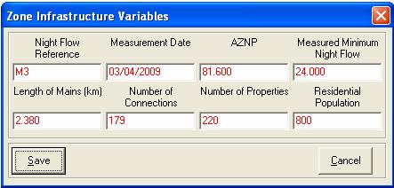
118 Jessy Alida Chipwaila 106

119 Appendix VI-c: Sadzi MNF Analysis Jessy Alida Chipwaila 107

120 Appendix VII: Bucket tests results and pipe network installed in 2001 (a) Bucket tests results Bucket size (litre) Airwing Sadzi Mtiya Average Average Bucket filling Bucket filling time size time size (mm:ss) (litre) (mm:ss) (litre) Average filling time (mm:ss) 20 1: : : : : : : : : : : : : : : : : : : : : : : : : : : : : : : : : : : : : : : : : : : :30 (b) Pipe network installed in 2001 Pipe Type Size (mm) Length (m) % type of Total GI , ,355 DI 200 1, , , PVC , , , ,750 Total Jessy Alida Chipwaila 108

121 Appendix VIII: Summary of pipe burst records for 2007 and 2008 Zone Area 2008 Jan Feb Mar Apr Jan Feb Mar Apr Type Sizes (mm) Notes Airwing Airwing PVC, AC Mtiya Mtiya PVC Sadzi Malonje Sadzi PVC, GI 32, , 25, 50, 63,90 Chizalo PVC 20, 25, 50 Thundu PVC, GI Mpunga PVC, GI 25, 50, , 75, Malonje PVC 20, 25, 63, 90 Habitat PVC, AC China mwali 20, 25, 50, PVC 50, 63 April 100mm AC 20, 25, 50 common. 160 mm X2 April , 150 mm GI bursts 90 mm burst in April 50 mm AC burst Mar08 90% bursts - 63mm Jessy Alida Chipwaila 109

122 Appendix IX: Some high bills between 2007 and Query cause Description Resolution No. 1 Wrong meter readings instead of Credit adjustment 2 Wrong meter readings instead of Credit adjustment 3 Wrong meter readings instead of Credit adjustment 4 45 m 3 instead of 28 m 3 Credit adjustment 5 Meter leakage SRWB not attend to problem after complaint 6 Broken valve SRWB not attend to problem after complaint 7 Computer feeding error 8 Computer feeding error 9 Computer feeding error 10 Error on posting of readings 11 Error on posting of readings Missed the actual meter readings Missed the actual meter readings instead of (50 m 3 error) instead of (45m 3 error) 54m 3 instead of 12 m3 Credit adjustment Credit adjustment of MK4872 Credit adjustment Credit adjustment Credit adjustment of MK3477 was made Credit adjustment of MK3127 Credit adjustment of Mk error at the recording instead of Credit adjustment of readings 13 Error at the collection of meter readings credit of MK Error at the collection instead of Credit adjustment of meter readings 15 Error at the collection instead of average 6-0 Credit adjustment of meter readings 16 Average charge Due to inaccessibility of meter. Average charge was high Credit adjustment of MK Wrong billing Billing a disconnected account Credit adjustment of MK444, error at the posting of readings instead of credit adjustment of MK153,000 Jessy Alida Chipwaila 110

123 Appendix X-a: Airwing Meter Inaccuracy Tests Meter Type Age Pressure (m) Volume tested(l) Flow rate (l/hr) Error% Kent Kent Kent Aquadis Kent Kent PSM Kent Kent PSM Kent Jessy Alida Chipwaila 111

124 Appendix X-b: Malonje Meter Inaccuracy Tests Meter Type Age Pressure (m) Volume tested(l) Flow rate (l/hr) Error% Kent Kent Kent PSM Kent Kent Kent Aquadis Kent Kent Kent Kent Kent Aquadis Kent Jessy Alida Chipwaila 112

125 Meter Type Age Pressure (m) Volume tested(l) Flow rate (l/hr) Error% Kent Jessy Alida Chipwaila 113

126 Appendix X-c: Sadzi Meter Inaccuracy Tests Meter Type Age Pressure (m) Volume tested(l) Flow rate (l/hr) Error% PSM Kent Kent PSM Kent Aquadis DN Kent Kent PSM Kent Kent PSM Kent Aquadis Kent Kent PSM Kent Kent Jessy Alida Chipwaila 114

127 Meter Type Age Pressure (m) Volume tested(l) Flow rate (l/hr) Error% Kent Kent Kent Kent PSM Kent Kent PSM Kent DN KentPSM Jessy Alida Chipwaila 115

128 Appendix X-d: Mtiya Meter Inaccuracy Tests Meter Type Age Pressure (m) Volume tested(l) Flow rate (l/hr) Error% Kent M Aquadis DN D08LA Kent A Kent below 600 meter not moving PSM Kent Kent PSM A Jessy Alida Chipwaila 116

129 Appendix XI: Map of Zomba Zomba km Jessy Alida Chipwaila 117

130 Appendix XII Zomba City water supply pressure zones Jessy Alida Chipwaila 118

131 Appendix XIII Research Pictures (a) (b) (c) (d) (e) (f) (g) (h) (a): Flow logger installed on a bulk meter (b): Pressure logger installed on a customer tap with a Tee (c): Pressure logger installed without Tee. (d): Manual pressure gauge inserted on customer tap (e): Plumber closing tank inlet valve to control overflow (f) Meter inaccuracy testing bench installed in series with customer meter under test. (g) Properly working tank meter (h) Vandalised tank meter. Jessy Alida Chipwaila 119