Air quality measurements and modelling

Transcription

1 Air quality measurements and modelling Massimo Stafoggia Dep. Epidemiology, Lazio Region Health Service, Rome, Italy

2 Air pollution The presence of toxic chemicals or compounds (including those of biological origin) in the air, at levels that pose a health risk. In a broader sense, air pollution means the presence of chemicals or compounds in the air which are usually not present and which lower the quality of the air or cause detrimental changes to the quality of life (such as the damaging of the ozone layer or causing global warming).

3 pollutants: any substance being present in the ambient air which might cause adverse effects on human health or on the environment in general. The ones included in the EU legislation are: - Sulphur dioxide (SO 2 ) - Nitrogen dioxide (NO 2 ) / Nitrogen oxides (NO x ) - Particulate matter (PM), inhalable (PM 10 ) and fine (PM 2.5 ) - Lead (Pb) - Ozone (O 3 ) - Benzene (C6H6) - Carbon monoxide (CO) - Polycyclic aromatic hydrocarbons (PAH) - Cadmium (Cd) - Arsenic (As) - Nichel (Ni) - Mercury (Hg) - Benzo(α)pyrene (B[α]p)

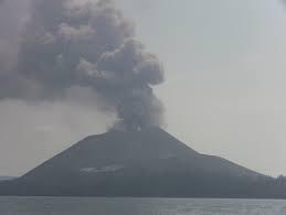
4 Agriculture (ammonia and methane) Air pollution: the sources Industrial activities (Sulphure oxides) Natural events (volcanic eruptions, erosion, pollen, desert dust ) Riscaldamento domestico Waste disposal (landfills, incinerators ) Transports (PM, nitrogen oxides)

5 Primary pollutants Substances emitted directly near the ground: SO 2 NO, NO 2 CO Benzene PAH Lead, heavy metals PM

6 Secondary pollutants Organic and inorganic substances: Not directly emitted by the sources near the ground Derive from chemical reactions which occur in the low atmosphere (in both gaseous and liquid phases) of pollutant substances otherwise not present in the air: Ozone NO 2 PM..

7 Technical Box 1 Level: concentration of a substance in the ambient air in a given time unit Concept of level (concentration) of a pollutant Es. let s consider NO 2 on the ground level 1) Isolate a volume V of air near the ground on a specific time unit t i and consider the mass M of NO 2 present there. The instantaneous concentration at t i is: C i = (M/V) i (µg/m 3 )

8 2) Repeat the instantaneous measure in following time units (ex. every minute for one hour), getting 60 measurements. If I am interested in the average hourly NO 2 concentrations, such level will be the hourly mean concentration of NO 2, i.e.: Hourly value = Hourly mean concentration = Sum (C i ) / N When we study the health effects of air pollutants, we are never interested in instantaneous values, but rather in average values, where the averaging time depends on the pollutant and the objective of the study (hourly, daily, annual, etc.)

9 Measurement methods Referent methods are defined, for each pollutant, by law For gaseous pollutants (SO 2, NO 2, O 3, CO, benzene) there are automated methods. For PM, the reference method would entail the weighting of a filter, therefore it would not be automated. However, law foresees equivalent methods which provide automatic measurements For other pollutants (PAH, Pb, ecc.) there are methods based on laboratory testing Figura Figura 4.2 Stazioni 4.3 Stazioni dell'agglomerato di misura nella di Roma Valle del Sacco

10 PARTICULATE MATTER v Complex heterogeneous mixture of solid and liquid components v Sources: Power plants and industry Motor vehicles Domestic coal burning Natural sources (volcanoes, dust storms) Secondary small particles from gases (nitrates and sulfates) 10

11 PARTICULATE MATTER: definitions A complex mixture of airborne solid and liquid particles, including soot, organic material, sulfates, nitrates, other salts, metals, biological materials. PM inhalable particles PM fine particles PM 10 -PM coarse particles PM ultrafine particles 11

12 Particulate matter

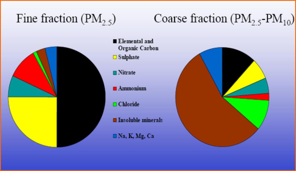
13 PARTICULATE MATTER: composition 13

14 Primary and secondary PM Fonte: Dati ambientali La qualità dell ambiente in Emilia-Romagna

15 Technical Box 2 Main cause for the presence of air pollutants in the air Emissions = any substance (solid, liquid or gaseous) introduced in the atmosphere which might cause air pollution Therefore, by definition, emissions are made solely by primary pollutants (ex. ozone is NOT emitted)

16 Transport and diffusion of pollutants emitted in the atmosphere Ground-level concentrations (Immissions) emissions

17

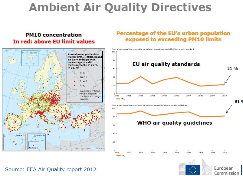
18 Law limits (D. UE 2008/50/CE)

19 PM 10 monitoring network in Italy

20 WHO AQG Summary (2005) Pollutant Averaging time AQG value EU standard (target or limit value) Particulate matter PM year 24 hour (99 th percentile) 10 µg/m 3 25 µg/m 3 25 µg/m 3 -- PM 10 1 year 24 hour (99 th percentile) 20 µg/m 3 50 µg/m 3 40 µg/m 3 50 µg/m 3 *** Ozone, O 3 8 hour, daily maximum 100 µg/m µg/m 3 *** Nitrogen dioxide, NO 2 1 year 1 hour 40 µg/m µg/m 3 40 µg/m µg/m 3 *** Sulfur dioxide, SO 2 24 hour 10 minute 20 µg/m µg/m µg/m 3 *** 350 µg/m 3 *** (1 hr) WHO levels are recommended to be achieved everywhere in order to significantly reduce the adverse health effects of pollution ***Permitted exceedances each year

21

22 Dispersion models Simulate, using fluidodynamic laws, emission, transport, dispersion and deposition of airborne pollutants, and also their chemical reactions They can be of different degrees of complexity depending on the sources they include, characteristics of the territory, source types and meteorological conditions. In general, they need as input: Quantities of emitted pollutants, their localization and how they are emitted Figura Figura 4.2 Stazioni 4.3 Stazioni dell'agglomerato di misura nella di Roma Valle del Sacco The structure (often 3D) of relevant meteorological parameters Characteristics of the territory (orografy, presence of lakes, land use, ecc.) sea/

23 Example. The modelling chain in Lazio Region Previsioni Meteorologiche Sinottiche (NCEP) Input Meteorologico Dati Geografici RAMS Gap SurfPRO Input Emissivo DATI EMISSIVI EMMA FARM Previsioni Inquinamento a scala nazionale (QualeAria) Campi di concentrazione Source: ARPA lazio

24 Air pollutants concentration maps Regional domain Metropolitan area of Rome

25 Land-use regression models They are aimed to predict pollutant concentrations in different spatial location by taking advantage of the spatial relationship between observations and land use characteristics They can be of different degrees of complexity depending on the data they include: road/traffic networks, population density, land cover, orography, etc. In general, they need as input: Observed measurements of the pollutant from one or more monitoring campaigns, with coordinates of the sites Figura Figura 4.2 Stazioni 4.3 Stazioni dell'agglomerato di misura nella di Roma Valle del Sacco Data on land use characteristics (and GIS expertise) Statistical expertise to develop a flexible model which relates land use data to the monitored pollutant(s)

26 1x1-KM FIXED GRID 307,635 cells

27 DATA OVERVIEW Daily PM concentrations Daily Aerosol Optical Depth (AOD) at 1x1-km Spatial parameters Population density Emissions from main inustrial plants Land-use characteristics Road network (distance from/meters of highways/main/minor roads) Others (elevation, impervious surfaces, geoclimatic zones, administrative layers, etc.) Spatiotemporal parameters Daily meteorology Monthly Normalized Difference Vegetaion Index (NDVI) at 1x1-km resolution Daily Planetary Boundary Layer (PBL) estimates at 10x10-km resolution Saharan dust

28 PM MONITORS 686 monitors PM 10 and PM 2.5

29 SATELLITE DATA: AOD and NDVI Annual average AOD, Italy 2010

30 POPULATION DENSITY

31 INDUSTRIAL EMISSION POINTS ~ 700 industrial sites

32 LAND-USE CHARACTERISTICS

33 ROAD NETWORK For each grid cell, and each of the three types of roads, two indicators: DISTANCE of the cell centroid from the closest road 2. DENSITY, as number of meters of roads in the cell

34 OTHER SPATIAL PARAMETERS Administrative layers Water bodies Geoclimatic zones Elevation Impervious surfaces

35 SAHARAN DUST Surface dust concentration maps - DREAM-BSC Surface dust, sulfate and smoke concentration maps NAAPS-NRL Back-trajectories - HYSPLIT Integrated dust load maps SKIRON simulations

36 PLANETARY BOUNDARY LAYER (PBL) Planetary boundary layer (PBL) is the lowest part of the atmosphere, extending from ground to the bottom of where cumulus clouds form. ECMWF provides hourly estimates of the PBL height at different times of the day (0.00, 6.00, 12.00, 18.00) and different spatial scales (0.125 x0.125, ~ 10x10-km for the purposes of this project). PBL data are provided at ~ 10km resolution. We attributed to each cell daily values at 0.00 and 12.00, based on proximity

37 METEOROLOGICAL DATA 630 stations: 140 airport stations 200 ARPA Lombardia, 200 ARPA-E, 33 ARPA Lazio, 24 Toscana, 33 Wunderground (2006 -)

38 METHODS 4-stage approach Mixed models Fit daily calibrations using data from pixels with co-located PM and AOD PM 10 ~ AOD + other spatio-temporal pars. (with mixed models) Use the calibration model fit to predict PM 10 in grid cells and days with AOD but without monitors Estimate PM 10 in cells with no available AOD data using spatial smoothing of nearby AOD and bimonthly regional patterns Stage 4 Improve Stage 1 PM 10 predictions by capturing additional sources of PM variation within grid cell due to very local sources. We collected data on small-scale spatial predictors defined around each monitoring station, and regressing them on the residuals of the CV stage 1 model

39 RESULTS: Italy map Fine spatial detail Mean predicted PM 10 from 5 µg/m 3 to 44 µg/m 3 Predicted PM 10 concentrations higher in the Po river valley, in major urban areas such as Rome and Naples, and close to the main industrial sites Lower on the Alpine and Apennine ridges

40 RESULTS: annual time trends

41 RESULTS: day-to-day variability Observed Stage 4 Stage 3 Daily PM 10 (µg/m 3 )