A comparison between Swat and a distributed hydrologic and water quality model for the Camastra basin (Southern Italy).

Transcription

1 University of Basilicata (Potenza) Dept. of Environmental Engineering and Physics (DIFA) A comparison between Swat and a distributed hydrologic and water quality model for the Camastra basin (Southern Italy). Aurelia Sole Donatella Caniani Ignazio Mancini

2 Objectives Use a distributed hydrologic model to improve understanding of the hydrology, water balance and water quality in the Camastra river basin (southern Italy). Make a comparison between Swat and the distributed hydrologic model results Test and validate model results. 2

3 Overview THE DISTRIBUTED MODEL Input data Theory SWAT MODEL Input data RESULTS AND DISCUSSION Comparison among SWAT, distributed model and observed daily discharge for 4 years of simulation 3

4 d d d d # Distributed model BASENTO RIVER Basilicata Potenza d 4 d 5 6 d d 4 7

5 Input data 5

6 Input data Input data for hydrologic distributed model DEM Flow direction grid Flow accumulation grid Streams Basin Burning in procedure Land use map 6

7 Digital Elevation Model Basin Area: 350 km 2 94 rows 102 columns 240 m grid Elevation (m) Quote (m) No Data Bacino del torrente Camastra Camastra river basin DEM 240 x 240 m 7

8 Dem recoditioning Digitized Stream network 8

9 Stream network extraction and basin delineation Bacino Camastra del torrente river basin Camastra Flow direction Flow Direction No Data Modello Flow accumulation Flow direction delle otto direzioni

10 Slope Pendenze Bacino Camastra del torrente river basin Camastra Slope map Carta delle pendenze 10

11 Land use and soils maps 11

12 ET R Distributed model The hydrologic and water quality distributed model, based upon a spatial discretization of the territory into elementary Q S Surfacesquare flow cells, schematises the main hydrological processes of degradation and transport of nutrients, performed on a control volume build on the t single cell. Q S = CP Q IN Subsurface flow Runoff ( θt θ0 ) ( θ θ ) De Smedt (2000) s 0 P Control Volume groundwater recharge Q OUT Subsurface flow C runoff coefficient P net precipitation (mm( mm) θ t soil moisture content at time t (mm) θ S saturated soil moisture content (mm) θ 0 residual soil moisture (mm) 12

13 Distributed model Runoff coefficient, C Q S = CP Runoff ( θt θ0 ) ( θ θ ) De Smedt (2000) s 0 13

14 Distributed model Default runoff coefficient Mallant e Feyen (1990) Land Use Slope Sand Loamy Sandy Silty Silt Loam Sandy Silty Clay Clay Sandy Silty Clay Clay (%) sand Loam Loam Clay Loam Loam Clay Loam Forest <0.5 0,03 0,07 0,10 0,13 0,17 0,20 0,23 0,27 0,30 0,33 0,37 0, ,12 0,13 0,15 0,17 0,19 0,22 0,25 0,28 0,32 0,36 0,40 0, ,17 0,19 0,21 0,23 0,25 0,27 0,29 0,32 0,35 0,39 0,44 0,50 >10 0,23 0,27 0,30 0,33 0,37 0,40 0,43 0,47 0,50 0,53 0,57 0,60 Grass <0.5 0,03 0,07 0,10 0,13 0,17 0,20 0,23 0,27 0,30 0,33 0,37 0, ,07 0,09 0,12 0,15 0,18 0,21 0,24 0,28 0,32 0,36 0,40 0, ,15 0,15 0,16 0,18 0,20 0,23 0,27 0,31 0,36 0,42 0,48 0,55 >10 0,20 0,21 0,22 0,24 0,26 0,29 0,33 0,37 0,42 0,47 0,53 0,60 Crop <0.5 0,23 0,27 0,30 0,33 0,37 0,40 0,43 0,47 0,50 0,53 0,57 0, ,27 0,31 0,34 0,37 0,41 0,44 0,47 0,51 0,54 0,57 0,61 0, ,33 0,37 0,40 0,43 0,47 0,50 0,53 0,57 0,60 0,63 0,67 0,70 >10 0,45 0,49 0,52 0,55 0,59 0,62 0,65 0,69 0,72 0,75 0,79 0,82 Bare Soil <0.5 0,33 0,37 0,40 0,43 0,47 0,50 0,53 0,57 0,60 0,63 0,67 0, ,37 0,41 0,44 0,47 0,51 0,54 0,57 0,61 0,64 0,67 0,71 0, ,43 0,47 0,50 0,53 0,57 0,60 0,63 0,67 0,70 0,73 0,77 0,80 >10 0,55 0,59 0,62 0,65 0,69 0,72 0,75 0,79 0,82 0,85 0,89 0,92 Impervius Area <0.5 0,32 0,35 0,37 0,39 0,42 0,44 0,46 0,49 0,51 0,53 0,56 0, ,35 0,37 0,38 0,40 0,42 0,45 0,47 0,50 0,52 0,55 0,58 0, ,40 0,41 0,41 0,42 0,44 0,46 0,49 0,52 0,55 0,59 0,64 0,69 >10 0,44 0,44 0,45 0,47 0,48 0,51 0,53 0,56 0,59 0,63 0,67 0,72 14

15 Distributed model ET R P RS Surface flow Q IN Subsurface flow Control Volume Q OUT Subsurface flow Soil moisture storage S t+ t = S t + F t E t RI t RG t dove S t+ = water content in the soil profile at time t+ t (mm), S t = total soil water content at time t (mm), F t = infiltration amount into the soil during the time t (Qin+P( Qin+P-RS) E t = actual evapotranspiration from the soil during the time t (mm), RI t RG t Percolazione = lateral in and out subsurface flow of the soil during time t (mm)( = groundwater recharge during time t (mm). 15

16 The subsurface flow starts when the soil water content exceeds the t field capacity. Subsurface lateral flow where R It = subsurface flow during time t (mm), S t = total soil water content at t time (mm), RI = max ( 0, c t i (S t -S ) ) C S c = soil water content at field capacity at t time (mm), c i = subsurface flow coefficient. The percentage of water that comes into the saturated zone can be b derived by the use of the Darcy law: where RG= groundwater recharge (mm/h), K= hydraulic conductivity (mm/h), grad(h)= hydraulic gradient RG = K grad(h) Distributed model 16

17 Distributed model The Irmay equation has been used in this study to calculate the groundwater recharge flow of the single cell: RG t = K t t = K s θ t θ n θ 0 0 α t = K s S S t S α t where: RG t K t K s = groundwater recharge at time t (mm), = hydraulic soil conductivity at t time (mm/h), = saturated hydraulic conductivity (mm/h), n = porosity α = index characterizing dimension and distribution of soil porosity θ t θ 0 soil moisture content at time t (mm) residual soil moisture (mm) 17

18 where: Potential evapotranspiration ET0 = kc p(0.46t + 8) k C = crop coefficient, T = average temperature of the last 10 days Actual evapotranspiration Distributed model (Blaney-Criddle equation) where: ET t = actual evapotranspiration (mm), ET 0 = potential evapotranspiration at time t (mm), b = empiric value, ET t = (1-e-b (qt θ t = soil moisture content at time t (mm), θ 0 = residual soil moisture (mm), b (qt-qo)/(qc qo)/(qc-qo θ C = soil moisture content at field capacity (mm). qo) ) ET 0 (Davies ed Allen, 1973) 18

19 SWAT data: soils layer 19

20 SWAT data: land use layer 20

21 SWAT data: DEM 1160 rows 1297 columns 20 m grid 21

22 SWAT: meteorological data Daily data of temperature, wind velocity, humidity and solar radiation) for eleven years (1990/2000) at 6 agro-meteorological stations have been collected from the Agro-meteorological Service of ALSIA (Development and Innovation in agriculture Agency of the Basilicata Region). Gage location Name LATITUDE LONGITUDE Elev. (m s.l.m.) Abetina Laurenzana Bosco Galdo Villa D'Agri Montecrispo Campo Maggiore Lupara Guardia Perticara S. Lucia Brindisi di Serra del Ponte Montagna Satriano

23 SWAT: meteorological data 23

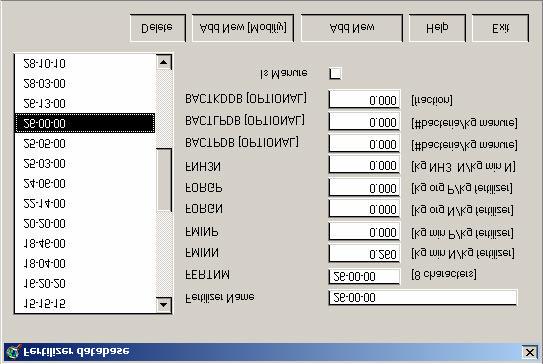
24 SWAT databases 24

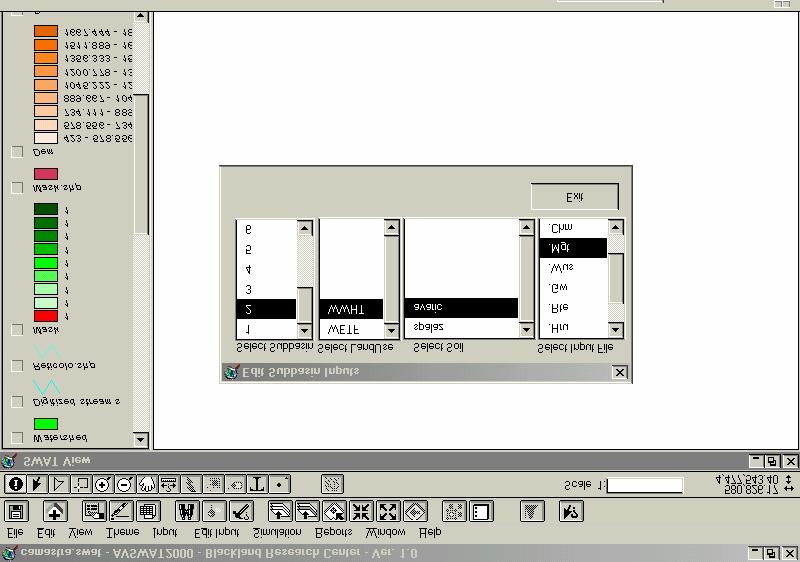
25 SWAT: management input data 25

26 Distributed model results Observed and simulated daily discharge Observed daily discharge Simulated daily discharge Q (m 3 /s) time (days) Correlation coefficient 0,77 Mean square error 2,91 26

27 Distributed model results 50 Observed and simulated daily discharge Observed daily discharge (m 3 /s) Simulated daily discharge (m 3 /s) Correlation coefficient 0,77 Mean square error 2,91 27

28 SWAT model results Observed and simulated daily discharge Observed daily discharge Simulated daily discharge Q (m 3 /s) time (days) Correlation coefficient 0,53 Mean square error 13,00 28

29 Distributed model results Observed and simulated daily discharge Observed daily discharge Simulated daily discharge Q (m 3 /s) time (days) Correlation coefficient 0,75 Mean square error 4,72 29

30 SWAT model results Observed and simulated daily discharge Observed daily discharge Simulated daily discharge Q (m 3 /s) time (days) Correlation coefficient 0,62 Mean square error 39,04 30

31 Distributed model results Observed and simulated daily discharge Observed daily discharge Simulated daily discharge Q (m 3 /s) time (days) Correlation coefficient 0,80 Mean square error 20,78 31

32 SWAT model results Observed and simulated daily discharge Observed daily discharge Simulated daily discharge Q (m 3 /s) time (days) Correlation coefficient 0,55 Mean square error 15,50 32

33 Distributed model results Observed and simulated daily discharge Observed daily discharge Simulated daily discharge Q (m3/s) time (days) Correlation coefficient 0,60 Mean square error 2,53 33

34 SWAT model results Observed and simulated daily discharge Observed daily discharge Simulated daily discharge Q (m 3 /s) time (days) Correlation coefficient 0,42 Mean square error 22,12 34

35 Conclusions and Discussion Results provide daily simulations of streamflow over the entire watershed, obtained with both models. Better results by using the distributed model even by using less accurate input data Difficulties: data availability and calibration of SWAT model Lack of soils parameters, potential evapotranspiration, solar radiation wind speed and relative humidity data. 35

36 University of Basilicata (Potenza) Dept. of Environmental Engineering and Physics (DIFA) A comparison between Swat and a distributed hydrologic and water quality model for the Camastra basin (Southern Italy). Aurelia Sole Donatella Caniani Ignazio Mancini

37 Simulation results Confronto Confronto tra tra i valori tra di idrogramma concentrazioni concentrazione simulato di azoto misurati e registrato nitrico e misurate determinati e attraverso l applicazione l del modello simulate proposto Concentrazione di Azoto (mg/l) Valori simulati Q (mc/s) (mg/l) 1,860 1,6 Portate Registrate Valori Sperimentali 50 1,8 Portate Simulate Risultato Elaborazione 1,4 1,6 1,2 40 1, ,2 0,8 1 0,6 20 0,8 0,4 0,6 0,2 10 0,4 0 0,2 0 01/12/ /03/ /06/ /09/ /01/ giorni giorni 0 0,5 1 1,5 Valori osservati sperimentalmente (mg/l) 37