Integrated Hydrology Model (InHM( HM): Development, Testing, and Applications

Transcription

1 Integrated Hydrology Model (InHM( HM): Development, Testing, and Applications DYNAS Workshop ``Numerical Modeling for Hillslope Hydrology'' INRIA Rocquencourt -- 6 to 8 December 24 Joel VanderKwaak 1,2 Keith Loague 2, Christopher Heppner 2, Adrianne Carr 2, Qihua Ran 2, Brian Ebel 2, Benjamin Mirus 2 1 ARCADIS G&M, San Francisco, California 2 Stanford University, Stanford, California

2 The Real World

3 Outline Motivation Numerical Model Laboratory scale eample Field scale eample Sub-catchment scale eample

4 Motivation Hydrology Spatial/temporal distribution of recharge and seepage Dynamics of variable source areas for stream flow generation Solute Transport subsurface vs overland pathways (mining, agriculture, urban runoff, atmospheric deposition, etc) chemically-based hydrograph separation Landscape evolution Erosion/deposition Dam removal Hillslope stability, pore pressures High conductivity features (fractures, macropores) Have to get the hydrology right in order to simulate transport processes

5 Research Philosophy Apply code to real problems Use real data, avoid calibration Honestly evaluate results Learn what doesn t t work (and why) Eperiment with alternative conceptualizations Open source the code so others can test, learn and contribute (see

6 InHM - Integrated Hydrology Model (insert name here model) Numerical model of flow and transport in multiple interacting continua Richards equation in subsurface (1d/2d/3d) Optional dual continua to represent fractures/macropores Optionally includes water/matri compressibility Leverett scaling of characteristic relationships Diffusion wave equation on land surface (1d/2d) Include depression storage (immobile water) Advection-dispersion dispersion equations (multiple species) Sorption Chain decay Air phase partitioning and diffusion Robust, general and efficient solution methods Control volume finite element with mied element types Optionally drop diagonal terms in finite elements Nodal properties (can be time variable) Primary variable switching for flow Nonlinear flu limiters for transport Implicit flow, Implicit/central transport, Optional adaptive implicit/eplicit solution Dynamically partition equations, solve reduced system Aggressive adaptive time stepping Node based assembly Full Newton solution using numerical derivatives Efficient iterative matri solver First-order coupling relationships Each system of coupled nonlinear discrete equations solved simultaneously

7 Coupled Continua Porous Medium Source/Sink Surface Source/Sink Porous Medium Storage Surface Storage Water and Solute Echange Flow and Transport within Porous Medium Macropore Storage Flow and Transport on Land Surface Macropore Source/Sink Flow and Transport within Macropores

8 Eample Coupled Matri Eample Coupled Matri Surface Element Porous Medium Element q9 d3 X 9 q8 d2 X 8 q7 d1 X 7 q6 h6 6 q5 = h5 5 q4 h4 4 q3 h3 X 3 q2 h2 X 2 q1 h1 X

9 Discrete Echange Relationships Flow: ( ) e e e Qs = Γ p sp ψs ψ p = Qp s e e ρwg zz As Γ sp = krw kp A µ a s : interface area w s 2D surface continuum (depth integrated) a s :characteristic interaction distance 3D porous medium continuum Transport: p ( ) Q = Λ C C = Q e e e s sp s p p D D D Q Λ = + e e sp * D e e As sp α ( φswτw ) D s w p A s as s

10 First Order Coupling Reqires definition of interface flu functions. 1D Darcy equation 1D advection-dispersion dispersion equation Coupling coefficients Consistent with coupling used in dual subsurface continua Large values make pressure head at land surface equal water depth Upstream weight interface relative permeability Harmonic weight interface saturation Coupling coefficients go to zero when there is no ponded water Our coupling coefficients functions of: interface geometry (e.g. thickness and area) system state (e.g. saturation) physical properties (e.g. permeability) Eliminates iteration between separate model components. Interface flues determined as part of solution Need to back-calculate calculate to get value Not defined a priori Evolve with spatially and temporally variable hydrodynamics

11 Eperimental Surface Functions Relative Water Depth: Pseudo-Saturation: Pseudo-Relative Permeability: ψ k = min 1, ma, ψ h 21 ( rel = ψ ψ ) rel s s S w rel rw S w Surface Saturation ψ s h s.2.1 linear functional Relative Water Depth

12 Flow Boundary Conditions Temporally and spatially variable Implemented as generic source/sink term Multiple boundary conditions can be simultaneously active All continua Specified flu (both rainfall and evaporation) Specified head or water depth Subsurface continua Drainage Specified gradient Etrapolated gradient Seepage Surface Continua Critical depth Tabulated depth-discharge discharge

13 Implementation Modular, structured, etensible Fortran95 Derived data types Dynamic memory management Modules defined by function Physics isolated from numerical methods Original development on Uni (SGi( SGi,, HP, IBM) Development currently on Windows and Linu Etending code to utilize potential of Linu clusters

14 Input InHM Components Finite element grid (internally or eternally generated) Physical constants and properties (can vary in time) Boundary conditions (variable in time and space) Solution parameters Generates an HDF5 input file Model Reads HDF5 input file Solves specified steady state or transient problem Writes results to HDF5 data file Output Reads HDF5 input and data files Performs statistical analyses Converts and normalizes units Writes visualization files (TecPlot( TecPlot,, GMS, etc)

15 HDF5 General purpose library and file format for storing and sharing scientific data C/C++/F95/Java interfaces Efficient storage and I/O Cross platform compatible Structured and self describing Large and varied user community Open source (free!)

16 Illustrative Eamples (Testing) Flow and transport at increasing spatial and temporal scales Laboratory ( Gillham( Gillham bo ) Small field site (Borden) Shallow slope 1 st -order catchment (R5)

17 Laboratory Scale Testing Pressure Head (cm) Saturation (cm) ' Rainfall' for 2 min across land surface (4.3 cm/hour) Bromide Tracer Monitoring Location 2 Discharge (cm 3 /min) Discharge C/C C/C (cm) 1 2 Time (min)

18 Finite Element Meshes Base Case Grid Fine Grid 1 Nodes: 3621 Subsurface Elements: 7 Surface Elements: 7 1 Nodes: Subsurface Elements: 28 Surface Elements: Elevation (cm) 6 4 Elevation (cm) Distance (cm) Distance (cm) Coarse Grid 1 Nodes: 936 Subsurface Elements: 175 Surface Elements: 35 8 Elevation (cm) Distance (cm)

19 1 9 8 Hydrographs Measured Refined Grid Base Case Coarse Grid Discharge (cm 3 /min) Time (minutes)

20 96 94 Hydraulic Heads Hydraulic Heads 12 1 Seconds Minutes 25 Minutes Seconds (cm) (cm) (cm) (cm)

21 Surface Water D(log 1 ) seconds 1.5 S -3 D(log 1 ) seconds 1.5 S -3 D(log 1 ) D(log 1 ) D(log 1 ) S 2 minutes 25 minutes (cm) S S

22 Tracer Concentrations Measured Refined Grid Base Case Coarse Grid C/C Time (minutes)

23 Lab Scale Conclusions Simulation of coupled surface-subsurface subsurface hydrologic response relatively easy. Simulation of conservative tracers relatively difficult. Surface tracer concentrations sensitive to 1 st order coupling relationship Discrete subsurface miing volume. Likely more. Futher work: Analysis of coupling sensitivity to form of 1 st -order coupling. Epansion of spatial scale and the physical meaning of parameters.

24 Borden Field Eperiment Distance (m) Elevation (m) Distance (m) Rainfall containing a conservative tracer applied for 5 minutes at 2 cm/hr Hydrologic response observed and measured Capillary fringe intersects land surface along stream ais (initial head about 22 cm below stream)

25 Field-Scale Testing Borden Field Eperiment (Abdul, 1985) Lab Eperiment (Abdul, 1985) 2 (m) (m) (m)

26 Field-Scale Testing Simulate field eperiment with two different finite element meshes: dz == 2 cm (lab scale) for 1 st 5 cm d, dy >> lab scale 1 st mesh == [2 5 cm] 2 nd mesh == [5 12 cm] All other parameters available measured or derived from lab eperiment.

27 Finite Element Meshes Nodes :21952 Subsurface Elements: Surface Elements: 2651 Nodes : Subsurface Elements: Surface Elements: X Y X 4 Z Y Z

28 Hydrographs Measured Simulated (coarse) Simulated (fine) Discharge (L/min) Time (min)

29 Tracer Concentrations Measured Simulated (coarse) Simulated (fine).7.6 C/C Time (min)

30 Tracer Mass Flu Measured Simulated (coarse) Simulated (fine) 6 C/C Time (min)

31 Field Scale Conclusions Highly nonlinear hydrologic response (another presentation) Surface discharge fairly easy to simulate. Tracer concentrations in discharge water fairly difficult to simulate. Concentration discrepancy appears to be greatest at low surface flows. Mass flu (Q*C) is simulated reasonably well. Horizontal spatial discretization relevant, but coarse mesh captured the essential physics.

32 Sub-Catchment Scale testing R5 Catchment Borden Field Site 4 3 (m) (m) (m) 3 4

33 R5 in the 8s

34 R5 Today

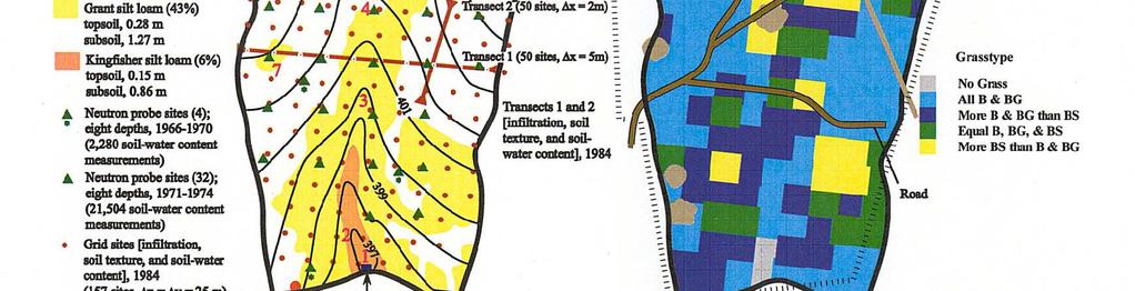
35 Data

36 Runoff

37 Event 68: Initial Conditions 41 Elevation (m) Distance (m) Distance (m) 45 Total Head

38 Rainfall Intensity (mm/hr) R5 Hydrographs 25 Streamflow (L/s) Observed VL LV Phase I Phase II Phase III Time (hours)

39 Event 68: Conditions at Peak Discharge 41 Elevation (m) Distance (m) Distance (m) 45 Total Head

40 Eample Coupled Response (animation)

41 Surface Saturation through Time 16 (d) e 14 Streamflow (L/s) (c) (b) (a) 12 d f 1 8 g c 6 h b Time (hours) (e) Saturation (f) (g) (h)

42 Runoff Generation (a) (b) 2 (c) 12 e Permeability (m 1 ) b Echange Rate (q ) / Rainfall Rate (q )

43 R5 Conclusions Used all measured data Guessed at initial water table location Active rainfall-runoff runoff mechanisms form a continua between infiltration-ecess (Dunne) and rainfall-ecess (Horton) Contributing area is a hysteretic function of rainfall- runoff history Hydrograph not perfect, but pretty good Low flow simulated less accurately Hydrologic response sensitive to representation of topography initial conditions

44 Continuous Simulations 5 Discharge (L/s) Event Time (days)

45 Catchment Scale Testing Mystery Catchment R5 Catchment (m) (m) (m) 5 4

46 Sediment Transport Multiple suspended species on land surface Solves reduced system of transport equations utilizing solution to fully coupled flow problem

47 Sediment Transport Component Test InHM Water Discharge (m 3 /s) Sediment Discharge (kg/s) Rate (.25 mm) Rate (.5 mm) Rate (.5 mm) 1 9 Discharge (m 3 /s).6.4 Kineros Water Discharge (m 3 /s) Sediment Discharge (kg / s) Rate (.25 mm) Rate (.5 mm) Rate (.5 mm) Sediment Discharge Rate (kg/s) Time (seconds)

48

49 Questions? Joel VanderKwaak Get the code -> Keith Loague