Hydrological analysis of the Evrotas basin, Greece

Transcription

1 Alterra is part of the international expertise organisation Wageningen UR (University & Research centre). Our mission is To explore the potential of nature to improve the quality of life. Within Wageningen UR, nine research institutes both specialised and applied have joined forces with Wageningen University and Van Hall Larenstein University of Applied Sciences to help answer the most important questions in the domain of healthy food and living environment. With approximately 40 locations (in the Netherlands, Brazil and China), 6,500 members of staff and 10,000 students, Wageningen UR is one of the leading organisations in its domain worldwide. The integral approach to problems and the cooperation between the exact sciences and the technological and social disciplines are at the heart of the Wageningen Approach. Alterra is the research institute for our green living environment. We offer a combination of practical and scientific research in a multitude of disciplines related to the green world around us and the sustainable use of our living environment, such as flora and fauna, soil, water, the environment, geo-information and remote sensing, landscape and spatial planning, man and society. Hydrological analysis of the Evrotas basin, Greece Low flow characterization and scenario analysis Alterra Report 2249 ISSN More information: M.M. Cazemier, E.P. Querner, H.A.J. van Lanen, F. Gallart, N. Prat, O. Tzoraki and J. Froebrich

2

3 Hydrological analysis of the Evrotas basin, Greece

4 This study has been carried out with support from the Dutch Ministry of Economic Affairs, Agriculture and Innovation. This research was also supported by the MIRAGE project, EC Priority Area 'Environment (including Climate Change)', contract number KB-code: Projectcode:

5 Hydrological analysis of the Evrotas basin, Greece Low flow characterization and scenario analysis M.M. Cazemier 1, E.P. Querner 1, H.A.J. van Lanen 2, F. Gallart 3, N. Prat 4, O. Tzoraki 5, J. Froebrich 1 1 Alterra 2 Wageningen University 3 Institute of Environmental Assessment and Water Research, Barcelona, Spain 4 Department of Ecology, Barcelona, Spain 5 Technical University of Crete, Greece Alterra-report 2249 Alterra Wageningen UR Wageningen, 2011

6 Abstract Cazemier, M.M., E.P. Querner, H.A.J. van Lanen, F. Gallart, N. Prat, R. Tzoraki & J. Froebrich, Hydrological analysis of the Evrotas basin, Greece; Low flow characterization and scenario analysis. Wageningen, Alterra, Alterra-report 2249, 90 p.; 57 Fig.; 22 Tables.; 40 Ref.; 8 Annexes This research increases knowledge of the hydrological processes acting in the Evrotas river basin (Greece) and performs a hydrological analysis and low flow characterization. The hydrological processes in the basin are modelled with SIMGRO (SIMulation of GROundwater and surface water levels). Flow status frequencies have been determined for every reach of the main stream network, i.e. dry, pools, connected, riffles or flood. Results show that approximately 60% of the stream network in spring and 50% of the stream network in summer is too dry to support a viable aquatic ecological community. A scenario analysis shows that the flow in the stream network has ceased considerably since the The perspective for 2050 is that the flow will cease further. Keywords: aquatic states, Evrotas, flow, Greece, seasonality, SIMGRO, temporary streams ISSN The pdf file is free of charge and can be downloaded via the website (go to Alterra reports). Alterra does not deliver printed versions of the Alterra reports. Printed versions can be ordered via the external distributor. For ordering have a look at Alterra Wageningen UR, P.O. Box 47; 6700 AA Wageningen; The Netherlands Phone: ; fax: ; info.alterra@wur.nl No part of this publication may be reproduced or published in any form or by any means, or stored in a database or retrieval system without the written permission of Alterra. Alterra assumes no liability for any losses resulting from the use of the research results or recommendations in this report. Alterra-report 2249 Wageningen, November 2011

7 Contents Preface 7 Summary 9 1 Introduction Aim and research questions Structure of the report 12 2 Research area description 13 3 SIMGRO preliminary model and low flow characterization SIMGRO model description SIMGRO application for the Evrotas river basin Schematisation Input data Groundwater Surface water Evapotranspiration Low flow characterization Temporary streams Aquatic states Discharge thresholds for the aquatic states Ecological status Seasonality and flow occurrence Fish communities present in the Evrotas river basin 27 4 Improvements of input data and model performance Reference scenario Transmissivity Irrigation Evapotranspiration Performance of the reference model Discharges Groundwater Determination of discharge thresholds Aquatic states frequencies for the stream network Sensitivity analysis Sensitivity of input data Sensitivity of discharge thresholds 51 5 Scenario analysis Historical scenarios Analysis historical scenarios 55

8 5.2 Future scenarios Scenario 2050 A en 2050 B Analysis future scenarios Discussion 65 6 Water Framework Directive 67 7 Conclusions and recommendations 69 Literature 71 Appendices 1 Main rivers 75 2 Upper, middle and lower reaches 77 3 Transmissivity 79 4 Geological map 81 5 Local instability 83 6 TRP s for spring dry periods 85 7 TRP s for all year dry periods 87 8 TRP s historical scenarios 89

9 Preface This report is the result of a thesis of the first author: a requirement for the MSc course Hydrology and Quantitative Water Management at Wageningen University. The research was carried out in the framework of the EU project MIRAGE. We received valuable information from experts in Greece and Spain and would like to thank Vasillis Papadoulakis and Nikolaos Nikolaidis for their help in this project. We could not have performed the climate change scenario analysis without the information provided by Iwan Supit of Alterra and thank him for provision of the climate data expected for Alterra-report

10 8 Alterra-report 2249

11 Summary The EU Water Framework Directive (WFD) pays very little attention to temporary rivers, because water quantity aspects (e.g. discharge) are not directly considered. However, water quantity has great impact on the ecological status of temporary rivers. The discharge of temporary rivers determines whether aquatic species will die out or can survive and recolonize river branches after a dry period. This situation depends on whether the river bed dries out completely or that pools remain, and how long these dry periods last. In this research the characteristics of temporary rivers has been investigated for the Evrotas river basin in Greece. The objective of the research is to increase knowledge of hydrological processes acting in the Evrotas river basin and to perform a hydrological analysis and low flow characterization in the context of the implementation of the Water Framework Directive. The Evrotas river basin is situated Greece, in the south of the Peloponnese. The basin consists of a valley between two mountain ranges and has an area of 2410 km 2. The hydrological processes in the basin are modelled with SIMGRO (SIMulation of GROundwater and surface water levels). The model is distributed and simulates regional transient saturated groundwater flow, unsaturated flow, actual evapotranspiration, irrigation, stream flow, groundwater and surface water levels as a response to rainfall, reference evapotranspiration, and groundwater abstraction. In this study, the performance of a preliminary model has been improved. This resulted in a better fit of the simulations against the measurements. Thresholds in the discharge have been identified to perform a low flow characterization: flow status frequencies have been determined for every reach of the main stream network, to define the possible states, i.e. dry, pools, connected, riffles or flood. The length and timing of the periods that the river reach is in the driest states (dry or pools) is critical for the development of aquatic ecological communities. Results show that approximately 60% of the stream network in spring and 50% of the stream network in summer is too dry to support a viable aquatic ecological community. A scenario analysis has been performed for the period 1900 to Three historical and two future scenarios were considered to assess the changes in the flow regime. The historical scenarios are based on changes in land use and irrigation. The future scenarios give an indication on the effects of climate change. The analysis shows that the flow in the stream network has ceased considerably since the 1980ties, mainly because from that period onwards, olives are irrigated. The perspective for 2050 is that the flow will reduce further, but the additional effects for the ecology are limited, and are especially in the spring period. Alterra-report

12 10 Alterra-report 2249

13 1 Introduction The Water Framework Directive (WFD) was implemented by the European Council in 2000 (WFD, 2000). The term ecological status was introduced in the WFD, defined as the ecological condition of an aquatic ecosystem based on biological, hydro-morphological and physicochemical elements (Vardakas et al., 2010). There are five categories classified by the WFD: high, good, moderate, poor and bad ecological status. The main objective of the WFD is to achieve good quality status for all water bodies by 2015 (Skoulikidis et al., 2010). The WFD pays very little attention to temporary rivers, because water quantity aspects (e.g. discharge regime) are not directly considered (Vardakas et al., 2010). However, water flow has great impact on the ecological status of temporal rivers. The discharge of temporary rivers determines whether aquatic species will die out or can survive and recolonize river branches after a dry period (Skoulikidis et al., 2010). This depends on whether the river bed dries out completely or that pools remain, and how long these dry periods last. Characteristics of a temporary river such as pools, connectivity and low discharge will be hereafter called low flow characteristics. Temporary rivers are common in Mediterranean countries (Skoulikidis et al., 2010). These waters are extremely sensitive to hydrological pressures (Vardakas et al., 2010). Management of Mediterranean river basins is a challenge, because there is little information on periods with low discharges. Basins are often prone to extreme conditions such as droughts, flash floods, desertification and forest fires (Andreadakis et al., 2008). Increasing amounts of ground and surface water are extracted for irrigation and further water scarcity is expected to increase due to climate change (Gasith, 1999; Vardakas et al., 2010) until A hydrological characterization, which can be used for systematic differentiation of the ecological stream types and reference conditions, was not available (Froebrich et al., 2010). However, during the past few years research is being conducted in the framework of different projects (Mariolakos et al., 2007, Gallart et al., 2008, Skoulikidis et al., 2010) to advance this knowledge. The MIRAGE EU project tries to improve the implementation of the WFD and the development of river basin management plans for Mediterranean catchments. The project will develop a framework to characterize the hydrological and ecological dynamics as well as to describe the measured impacts for the specific conditions of temporary streams (Froebrich et al., 2010). MIRAGE focuses on several river basins in the Mediterranean, and will test results and scenarios. One of these river basins is the Evrotas catchment in Greece, located in the south of the Peloponnese. The main environmental problem in the Evrotas river basin is the overexploitation of the water resources and therefore the dry circumstances in the river basin (Vardakas et al., 2010). As a result, fish populations are under stress and the Evrotas river changed from permanent to temporary during the past few decades. Assessment of the hydrological states in the basin and the consequences for the aquatic ecology is needed for a successful implementation of the WFD. 1.1 Aim and research questions The aim of the research is to increase knowledge of hydrological processes acting on the Evrotas river basin and to perform a hydrological analysis and low flow characterization in the context of the implementation of the Water Framework Directive. Alterra-report

14 This led to the following research questions: How can the existing SIMGRO (SIMulation of GROundwater and surface water levels) model of the Evrotas basin be improved to approach reality as closely as possible? What are the current flow and low flow conditions in the Evrotas basin? How is the WFD implemented in the Evrotas basin? What is the sustainable water use in the Evrotas basin? 1.2 Structure of the report In Figure 1.1, an outline is given of the steps carried out in this study. In the second Chapter, the research area is described. The main characteristics are given, along with information on the river flow and the aquatic organisms. In Chapter 3, the preliminary model developed by Vernooij et al. (2011) and the relevant input data are explained, as well as the methods for the low flow characterisation. This chapter includes information on temporary rivers, aquatic states and the fish communities in the river basin. In Chapter 4, the changes made to the input data and model performance are described. Furthermore, the model performance is shown and a low flow characterization is performed after identifying threshold values for different aquatic states. The consequences for the aquatic ecology are given. The last part of Chapter 4 consists of a sensitivity analysis. Chapter 5 includes a scenario analysis. The model results and low flow characterization were compared for historical and future scenarios. With available climate projections, future climate change in the Evrotas river basin is simulated in two scenarios for the year With historical data collected by Vernooij et al. (2011) an analysis of the changes in the hydrological regime during the past century is made through historical scenarios. Subsequently in the final chapter the consequences for the Water Framework Directive will be discussed followed by the conclusions and recommendations. Figure 1.1 Flow chart representing the activities carried out in this research 12 Alterra-report 2249

15 2 Research area description The Evrotas river basin is situated Greece, in the south of the Peloponnese (Figure 2.1). The basin consists of a valley between two mountain ranges. The total height difference is 2400 m, with the sea level as the lowest point. The basin has an area of 2410 km 2. The climate in the area is Mediterranean, which is characterised by dry, hot summers and wet, cool winters (Andreadakis et al., 2008). The average annual temperature in the basin is 16 C and the average precipitation is 803 mm per year, both for the period (Vardakas et al., 2010). The subsurface of the area consists of limestone (49%) and schist (29%) (Vernooij et al., 2011). The valley is filled with fluvial sediments of different age. In Figure 2.2 the rock types at the surface of the river basin are shown. The alluvial deposits are present in the valley, where the main river flows (Figure 2.2). Figure 2.1 Location of the Evrotas river basin (Vernooij et al., 2011). Alterra-report

16 Figure 2.2 Rock types at the surface of the river basin The land use in the basin consists for 61% of natural and semi-natural terrain. A further 38% is cultivated land, where predominantly oranges and olives are grown (Figure 2.3). The remaining land surface is occupied by urban areas (1% of the river basin). Figure 2.3 Current land use in the Evrotas river basin 14 Alterra-report 2249

17 The largest city in the river basin is Sparta, with approximately inhabitants. The location is shown in Figure 2.4. Close to this city the only waste water treatment plant in the river basin is located. The effluent is discharged into the Evrotas river (Vernooij et al., 2011). Figure 2.4 A few important points in the Evrotas river basin The Evrotas is the main river, with a total length of 90 km. Because the river basin partly has a karstic subsurface (limestone), there are many springs that give water throughout the year (Vardakas et al., 2010). These are mainly found in the north and north western part of the basin (Andreadakis et al., 2008). There are different surface water abstraction points in the Evrotas river basin and numerous municipal and private groundwater abstractions (an estimated 3500) for irrigation purposes (Skoulikidis et al., 2011). Overexploitation of the available groundwater has caused groundwater levels to drop during the past decades. There are permanent weirs in the basin redirecting water to areas under irrigation, while during the late spring and summer many more temporary weirs exist, diverting even more water from the river (Skoulikidis et al., 2011). Groundwater and surface water abstraction is illegal in the area from the bridge in Sentenikos (Figure 2.4) to the mouth of the Evrotas river up to 300 m from the river banks. However, this is done illegally and is not enforced by the local authorities (Skoulikidis et al., 2008). The basin currently represents a typical Mediterranean stream system despite its karstic features (Vardakas et al., 2010). One of the main characteristics of such a system is that the rivers experience high (peak) flows in winter and low flows during summer. Part of the stream network in the Evrotas basin does not have surface water flow during the summer period since only a small part of the precipitation (6%) occurs in summer, which mostly evaporates. The no-flow periods in the Evrotas river basin have increased in stream length and duration during the past half century. This is mainly caused by the expansion of agricultural areas and irrigation practices. Also, there has been influence of climate change leading to drier conditions and more extreme weather (Skoulikidis et al., 2010). The drying of the river affects also the surrounding areas. The number of wildfires increases (Andreadakis et al., 2008). Surface runoff generally increases after a wildfire, because evaporation and infiltration decreases (Andreadakis et al., 2008). Also, desertification is intensified after a wildfire (Blake et al., 2008). Alterra-report

18 The river basin also regularly experiences events with high rainfall intensities after a dry period. Due to the dry crusted conditions the system responds very fast. This leads to flash floods with high discharges carrying large amounts of debris and sediments (Moraetis et al., 2010). Despite the dry conditions in the Evrotas river basin, the streams still have a high and unique biodiversity. There is a large variety of flora and fauna present, of which many endemic species (Vardakas et al., 2010). The river hosts five native fish species, of which two cannot be found in any other river basin. An ecological status assessment has been conducted by Vardakas et al. (2010). They concluded that the physicochemical status and the biological status for macro invertebrate fauna was good. However, for ichthyofauna 53% of the sample sites had a poor biological status. They also concluded that fish-based ecological assessments can reveal remaining effects of hydro-morphological disturbances. The hydro-morphological status varied greatly through the river basin (Vardakas et al., 2010). This is explained by anthropogenic alterations to the river bed in parts of the river basin, like extended farmlands, flood works, extraction of gravel and straightening of river courses (Vardakas et al., 2010). 16 Alterra-report 2249

19 3 SIMGRO preliminary model and low flow characterization In this chapter the SIMGRO model is described. Thereafter the application of SIMGRO for the Evrotas river basin will be discussed along with the major input data. Furthermore, the methods used for the low flow characterisation will be elaborated. 3.1 SIMGRO model description To predict the effect of measures on a complex river basin like the Evrotas, it is necessary to use a combined groundwater and surface water model. SIMGRO (SIMulation of GROundwater and surface water levels) is a distributed parameter model that simulates regional transient saturated groundwater flow, unsaturated flow, actual evapotranspiration, sprinkler irrigation, stream flow, groundwater and surface water levels as a response to rainfall, reference evapotranspiration, and groundwater abstraction (Figure 3.1). To model regional groundwater flow, as in SIMGRO, the system has to be schematized geographically, both horizontally and vertically. The horizontal schematization allows different land uses and soils to be input per node, to make it possible to model spatial differences in evapotranspiration and moisture content in the unsaturated zone. For the saturated zone, various spatially-distributed subsurface layers are considered; for the surface water, the streams are simplified into one reservoir per subcatchment (Figure 3.1). For a comprehensive description of SIMGRO, including all model parameters, see Querner (1997) or Povilaitis and Querner (2006). Figure 3.1 Schematization of the hydrological system modeled with SIMGRO (Querner and Van Bakel, 1989) The model is used within the GIS environment ArcView. A user interface, AlterrAqua, serves to convert digital geographical information (soil map, land use, watercourses, etc.) into input data for the model. The results of Alterra-report

20 the modelling are visualised and analysed together with specific input parameters. AlterrAqua was built according to Dutch environmental conditions, which have to be adjusted when modelling a catchment with a different climate, land use and subsurface. In SIMGRO the finite element procedure is applied to approach the flow equation which describes transient groundwater flow in the saturated zone. A transmissivity is allocated to each nodal point and aquifer to account for the regional hydrogeology. The unsaturated zone is represented by means of two reservoirs, one for the root zone and one for the subsoil (Figure 3.1). The calculation procedure is based on a pseudo-steady state approach. If the equilibrium moisture storage for the root zone is exceeded, the excess water will percolate towards the saturated zone. If the moisture storage is less than the equilibrium moisture storage, then water will flow upwards from the saturated zone (capillary rise). The height of the phreatic surface is calculated from the water balance of the subsoil below the root zone and the saturated flow equation, using a storage coefficient. The equilibrium moisture storage, capillary rise and storage coefficient are required as input data and are given for different depths to the groundwater. Actual evapotranspiration is a function of the reference evaporation, the crop and moisture content in the root zone. To calculate the actual evapotranspiration, it is necessary to input the measured values for net precipitation, and the potential evapotranspiration for a reference crop (grass) and woodland. The model derives the potential evapotranspiration for other crops or vegetation types from the values for the reference crop, by converting it with known crop factors. The surface water system usually consists of a natural river and a network of small watercourses, lakes and pools. It is not feasible to explicitly account for all these watercourses in a regional simulation model, yet the water levels in the smaller watercourses are important for estimating the amount of drainage and the water flow in the major watercourses is important for the flow routing. The solution chosen in SIMGRO is to model the surface water system as a network of reservoirs. The inflow into one reservoir may be the discharge from the various watercourses, ditches and surface runoff. The outflow from one reservoir is the inflow to the next reservoir. For each reservoir, input data are required on two relationships: 'stage versus storage' and 'stage versus discharge'. For the interaction between surface water and groundwater, there are four different categories of water courses (related to its size) to simulate the drainage. It is assumed that three of the subsystems - ditches, tertiary watercourses and secondary watercourses - are primarily involved in the interaction between surface water and groundwater. A fourth system includes surface drainage to local depressions. Snow accumulation has been accounted for in the model: it is assumed that snow accumulation and snow melt are related to the daily average temperature (degree-day approach). When the temperature is below 0 C, precipitation falls as snow and accumulates. At temperatures between 0 C and 1 C, both precipitation and snow melt occur: it is assumed that during daylight hours the precipitation falls as rain, whereas precipitation falling during the night accumulates as snow (and the melt rate is 1.5 mm water per day). When the temperature is above 1 C, the snow melts at a rate of 3 mm/day per degree Celsius. 3.2 SIMGRO application for the Evrotas river basin The preliminary SIMGRO model was developed for the Evrotas river basin by Vernooij et al. (2011). This chapter gives a short description of the SIMGRO model developed for the Evrotas basin. For a detailed explanation of the setup of the model readers are referred to (Vernooij et al., 2011). 18 Alterra-report 2249

21 3.2.1 Schematisation The modelled area of the Evrotas river is given in Figure 3.2. The area is approximately km 2. The basin is covered by a network of more than nodes in which each node represents a part of the groundwater system. Nodes are spaced about 400 to 600 m apart. As is shown in Figure 3.2 there is a denser network of nodes, spaced 100 m apart, in an area in the northern part of the catchment. This is a relic of the original purpose of the model, which focussed on this area. Also a number of extra piezometers have been placed there in Figure 3.2 Schematization of the modeled area The time step of the groundwater model is one day. However, the surface water sub model performs several computational time steps during one time step of the groundwater sub model. The dynamics of surface water movement are much faster than those of groundwater movement. Therefore both sub models have their own time step. The time step of the surface water sub model is 0.05 days, and the time step of the groundwater sub model is one day. Groundwater levels remain constant during the time steps of the surface water sub model. After one day the groundwater sub model updates the groundwater levels using the state of the unsaturated zone and the surface water zone at that point in time. Alterra-report

22 3.3 Input data In this Chapter, the main input data used for the preliminary model are discussed. The main input data concern groundwater, surface water and evapotranspiration. For further details readers are referred to Vernooij et al. (2011) Groundwater The subsurface in the basin is built up with different schist and limestone layers. The layers were folded during orogenies. At places, these are covered by several alluvial layers. To schematize these layers every node has three layers in the saturated zone: the phreatic aquifer (layer 1), an aquitard (layer 2) and a deep aquifer (layer 3). For every node, layers 1 and 3 have a thickness and a conductivity determining the transmissivity. Layer 2 has a fixed thickness and a hydraulic resistance. Further details are given in Chapter The phreatic aquifer receives water from the unsaturated zone through percolation and loses water to the unsaturated zone through capillary rise. This aquifer also drains to the surface water and might receive infiltration water. The aquitard is not incorporated in the model based on hydrogeology, but is necessary for the numerical stability of the model. In the aquitard there is vertical flow between the two aquifers. It is assumed that the third layer, the deep aquifer, is overlying the hydrological base and that there is no exchange of water between that layer and underlying layers. There are a number of groundwater wells of which there are groundwater level measurements available. The locations of the wells are shown in Figure 3.3. These groundwater wells are often also used for irrigation purposes. Figure 3.3 The main rivers on the Evrotas river basin with the locations of the groundwater wells. With the names the layer numbers are given. Layer 1 is the phreatic aquifer; layer 3 is the lower aquifer 20 Alterra-report 2249

23 3.3.2 Surface water Based on the main streams considered for the surface water modelling, the basin was divided into 544 subcatchments. These subcatchments consist of the reservoirs mentioned in Chapter 3-1. The size of the subcatchments, they are shown in Figure 3.4. Due to lack of information but based on a limited number of photos, the width of the river of the headwaters is set to 3 m, the width of the middle reaches is 10 m and the main river is assumed to be 30 m wide (Vernooij et al., 2011). The spatial distribution of the sizes can be found in Appendix 1. Figure 3.4 Subcatchments identified in the Evrotas river basin The network of rivers, streams, channels and ditches is dense, as is shown in Figure 3.5. All these water courses are used to simulate the interaction between surface water and groundwater. For each node a drainage resistance and the difference in level between the simulated groundwater and pre-defined surface water are used to calculate the water flow (either drainage or infiltration). In Figure 3.6 the locations of the gauging stations in the river basin are shown. The discharge data from these stations are used to compare against model output. There are no measurements of surface water levels. Alterra-report

24 Figure 3.5 Network of watercourses in de Evrotas basin Figure 3.6 Main rivers in the basin with the locations of the gauging stations 22 Alterra-report 2249

25 3.3.3 Evapotranspiration In the Evrotas river basin, the evaporation has been measured using a 'Class A evaporation pan' (Vernooij et al., 2011). This technique combines the effects of temperature, humidity, wind and heat (Allen et al., 1998). The measurements have been converted to reference crop evapotranspiration (ET0) by the Greek Meteorological Service through multiplying the values with a pan coefficient. The pan coefficient varies from 0.35 to 0.85 for Class A evaporation pans (Allen et al., 1998). SIMGRO uses the ET0 to calculate the actual evapotranspiration through the following steps. First, the potential evapotranspiration is derived from the reference crop evapotranspiration using crop factors. A crop factor is a correction factor containing all variation of evapotranspiration with crop type, growth stage or management practice. Secondly, the actual evapotranspiration of each crop is determined in the model depending on the moisture content in the root zone. 3.4 Low flow characterization In this Chapter, temporary stream classification and aquatic states are described. Furthermore, an elaboration will be made on the methods used for the low flow characterization. Finally, additional information on the fish communities will be given, since they are important for the low flow characterization Temporary streams The term temporary rivers is generally used as the term for all non-permanent, intermittent, ephemeral and episodic streams (Moraetis et al., 2010). Several classifications for the degree of non-permanence have been made to assess the hydrological regime. A few examples are given here. Poff (1996) has defined three major classes of non-permanent flow: more than 90 days per year no flow is called harsh intermittent (HI), more than ten days per year no flow is intermittent flashy (IF) or intermittent runoff (IR), depending on the variation in daily discharge and frequency of floods and periods of low discharge. Streams with less than ten days per year no flow are considered permanent. Kennard et al. (2010) have made a more specific classification. They divided the flow regime into twelve classes. Class 1 through 4 are permanent rivers of varying degrees and class 4 through 12 are temporary streams and rivers. The last group is further subdivided into rivers that have short no-flow periods (class 5-8) and rivers often have no discharge (more than six months per year, class 9-11). However, for most of these classifications ecological effects are not taken into account: there is only a hydrological basis (Gallart et al., 2011). The length of the no-discharge period is critical to aquatic life and the presence, size, durability and physicochemical conditions of individual pools remaining are equally important. Therefore, Gallart et al. (2011) have developed a classification for flow regimes based on the consequences for the ecology. The states they propose are: Permanent (P): there is no influence of the hydrological regime on the ecology with respect to low flows. Intermittent-pools (IP): there is enough flow for the development of aquatic communities, but in summer the flow ceases and pools remain. The communities are impoverished but are able to recover. Intermittent-dry (ID): streams dry out completely in summer. However, in spring there is development of some communities and therefore ecological quality assessment may remain possible in some cases. Episodic-ephemeral (E): water flow is occasional and pools are short lived. There are some resilient organisms found but community development is impossible. Ecological quality assessment is not possible with regular methods. However, further specifications are needed to quantify the states mentioned above. These will be elaborated in the following paragraph. Alterra-report

26 3.4.2 Aquatic states The analysis of complex temporal patterns of occurrence of dry periods is simplified by introduction of the Aquatic States (Gallart et al., 2011). The aquatic states consist of a number of aquatic habitats available on a particular stretch of river in a certain time of year depending on the amount of flow. Such analyses can be done using daily discharges or monthly averages. The analysis determines in what state every river reach is. The different aquatic states are (Gallart et al., 2011): Flood: high discharges causing stream bed movement and drifting away of macro fauna. This is not the main focus of this research and will therefore not be elaborated upon. However it is worth mentioning that flash floods do occur in the basin creating a short but strong disturbance of the aquatic communities. These flash floods are of a too short time scale to be visible in the monthly summaries of aquatic states. Riffles: stream reaches in the Evrotas basin have a rocky subsurface because of which the bed of the river is not smooth but varies between deeper parts followed by shallower parts with small rapids. The shallow parts with relatively high flow velocities are called riffles and this state is thus apparent if the discharge is sufficient to create these riffles. This state is the predominant state of permanent rivers. Connected: if the flow velocity is not sufficient to create riffles in the shallow parts of the stream bed, the aquatic state is called connected. The pools in the river are still connected but there is no significant flow visible. Pools: if discharge ceases, the different pools or deeper parts of the river are not connected anymore. However, there may be some subsurface flow that connects the pools. The pools are important for the aquatic fauna but the quality of the habitat deteriorates fast with time. Large temperature fluctuations and depletion of oxygen create harsh conditions in which not many organisms can survive (Lake, 2003). Dry: the pools dry out and most of the streambed falls dry. The remaining wet parts in the alluvium are the remaining places for aquatic organisms to seek refuge. The flow is averaged per month to create an Aquatic States Frequency Graph (ASFG). This time scale gives an average image of the daily fluctuations in river discharge (Gallart et al., 2011). An example of an ASFG is shown in Figure 3.7. It shows, for a reach in the river basin, which percentages of the aquatic states are present per month. This sample ASFG shows that, from July until December, the stream bed can be dry. For October, this is the case in 30% of the time. Figure 3.7 Example of an aquatic states frequency graph 24 Alterra-report 2249

27 3.4.3 Discharge thresholds for the aquatic states Threshold values are needed to construct the Aquatic States Frequency Graphs (ASFG's). These are fixed discharge values, which determine the boundaries between the dry state, if there are pools, when the river is connected, when there are riffles and when there is flood. It is important, in establishing these thresholds, to ensure that the boundaries between the aquatic states are well based. Only then the ASFG s can be used for analysis and to derive consequences for the aquatic ecology. The water depth at low flows is also important, because especially fish need a minimum water depth to be able to survive. The river width is highly variable and can vary extremely from low flow to flood events. In this hydraulic flow analysis, focussing on the lower flow states, the width of the actual flow section is varied according to the assumed sizes of the rivers (3, 10 or 30 m as shown in Appendix 1). Table 3.1 gives the assumed river widths for the different aquatic states. In this way, threshold values are set for the water depth, which are limits for the development of aquatic ecology in the river. These thresholds in water depth are then converted to discharges by the model, allowing the discharge regime to be divided into the various aquatic states as discussed in Chapter Table 3.1 Widths considered for the low flow conditions and based on the assumed sizes of the rivers (3, 10 or 30 m, Appendix 1) Aquatic state Wetted width (stream 30 m) Wetted width (stream 10 m) Wetted width (stream 3 m) Dry 2 m 2 m 2 m Pools 2 m 2 m 2 m Connected 2 m 2 m 2 m Riffles Flood 5 m 20 m 3 m 5 m 2 m 3 m The threshold values in terms of water depth are selected using information about the fish sizes (Chapter 3.4.6) and are calibrated later on (Chapter 4.3). Fish are used here because they can relatively easy be used to indicate minimal, but sufficient water depths. The corresponding discharge values are calculated using the Manning formula (Chow, 1959). With this formula, a water depth can be determined, which matches the discharges calculated by the model for all rivers in the basin. The formula used is shown in Equation 3-1. It is assumed that the river has a rectangular cross section. Q 1. d. b. R n 2 3. S 1 2 = Equation 3-1 Where: Q = discharge (m 3.s -1 ) n = Manning coefficient (s.m 1/3 ) d = water depth (m) b = stream width (m) R = hydraulic radius (m) S = slope (m/m) The height of the peak discharges varies strongly between the main river and the headwaters. Therefore there are additional conditions built in for the flood threshold. First, this threshold value has to be exceeded by at least 2% of the discharges. In addition, the model checks whether the threshold for flood is larger than the threshold for riffles. The value cannot be smaller, because then the aquatic state flood will be reached with Alterra-report

28 lower discharges than the aquatic state riffles. If so, the threshold for flood is put to the maximum water depth that the model has calculated. The stretches of river where this occurs are in fact very dry so the thresholds will be rarely exceeded at all. The aquatic state with riffles is then the state with the highest water levels and flood does not occur Ecological status For the viability of an aquatic ecosystem in an intermittent river there are two issues important: how long a river falls dry each year and whether the occurrence is seasonal (Lytle and Poff, 2004). On these two quantities the potential for a viable aquatic community is based (Gallart et al. 2011). If a dry period in a river is predictable for an aquatic community, it allows the community to adapt and therefore increase their survival chances during a dry spell. The longer the dry period is, the less species can survive, and only resilient species remain that have adapted to the circumstances (Lake, 2003). If the dry periods occur in the same period each year, the aquatic community can adapt more easily and survival chances increase (Magalhaes et al., 2007). Prat (pers. comm.) states that in the spring period from March 21 until June 21, a river reach has to flow for more than 61 days. Therefore, a dry stream bed with pools periods may not last longer than 31 days in this period. The low flow conditions are important for the ecosystem in the river because most species reproduce in this period to survive the summer as an egg or larva. It is disastrous for the ecology if in this period the river is dry this long. In these conditions the ecological status cannot be assessed, because the aquatic community cannot be organized at the adequate level, the species richness will be low and only tolerant species will be present. If the situation is deteriorated by human influence and the river previously did have flow for more than two months in the past the ecological status is poor. Furthermore it is necessary to set an ecological limit to the duration a river reach experiences a dry stream bed during the dry period in summer. If a reach is dry for longer than 92 days or three months, if this is caused by a natural regime, the ecological status can only be measured using terrestrial invertebrates. However, if this regime is human induced the hydrological status is poor and consequently the ecological status is as well Seasonality and flow occurrence In addition to the analysis with the ASFG (section 3.4.2), Gallart et al. (2011) propose two other indicators which can be used to assess impacts on ecology. These are the Flow occurrence (Mf) and the Seasonal predictability (Sd 6 ) (Gallart et al., 2011). The flow occurrence, Mf, is the method used to describe the degree of drying up. This is a measure for the flow permanence given as the average percentage per year there is flow. The seasonal predictability indicator, Sd 6, is a measure developed by Gallart et al. (2011) to be able to give a characterization of the dry periods. The equation for the Seasonal predictability is shown in Equation = - Fd i Fd / j Sd Equation 3-2 Where: Sd 6 = seasonal predictability Fd i = multi-annual frequencies of no-flow for six contiguous months Fd j = multi-annual frequencies of no-flow for the next six contiguous months 26 Alterra-report 2249

29 This method uses the probability for the river to fall dry for each month and always divides the average of six months by the average of the following six months. This is performed for all combinations of the consecutive months: 1 through 6 divided by 7 through 12 followed by 2 through 7 divided by 8 through 1, and so on. The smallest value is chosen as the largest difference between the sets of six months. If there is always flow, the seasonal predictability Sd 6 cannot be calculated. In these cases, the Sd 6 is arbitrarily set to one, because the predictability of a non-dry period is obviously 100%. The seasonality and flow occurrence are plotted in one graph, called a Temporal Regime Plot (TRP). For an example, see Figure In a TRP, the relationship between the predictability of dry state periods and the occurrence can be visualized Fish communities present in the Evrotas river basin In rivers where the flow frequently diminishes to pools or less, invertebrate and fish species are adapted accordingly, especially if the seasonal dry periods occur at fixed times in the year (Capone et al., 1991). Invertebrates can get through dry periods as egg or larva. Fish often seek permanent springs, lakes or the sea to get through dry periods. This also occurs in the Evrotas basin (Skoulikidis et al., 2011). For fish the most important part of their habitat is the wet surface. The conditions for the size of this surface vary per species (Clausen, 2004). Often a certain water depth is needed for residence and a minimum water depth for passage. At low flows, the wetted perimeter decreases, causing the habitat for aquatic life to decrease. The river can dry out so that the connection between the pools disappears. This environment may be inappropriate for some species. In addition, the temperature, oxygen and ph will fluctuate more in the pools so that the environment in the pools becomes a harsh environment to survive in and one species is better adapted to these conditions than the other (Clausen, 2004). Therefore it is necessary to know which fish species live in the basin of the Evrotas. The Evrotas river basin hosts a number of fish species, of which three are unique and occur nowhere else (Vardakas et al., 2010). These are Squalius keadicus, Pelasgus laconicus and Tropidophoxinellus spartiaticus. The other species, Anguilla anguilla, Gambusia holbrooki and Salaria fluviatilis, are also found in other Mediterranean catchments. The specifics of these six species are given in Table 3.1 to give an indication of the habitats the different species need. In the first half of the 20 th century, the native fish species occurred in most of the stream network. However, they have gone extinct in the majority of the tributaries (Skoulikidis et al., 2010). Because of the habitat specifications (Table 3.1), the fish populations in the basin are affected in different ways by the low flows in summer. Skoulikidis et al. (2011) have kept track of the fish stocks in the dry year 2007, 2008, and This showed that the minimal discharges in summer create conditions that are favourable for stagnophilic species (preferring stagnant water) and unfavourable for rheophilic species (preferring fast flowing waters), because low water levels cause a decrease in their favoured habitats. During the dry year of 2007 the numbers of the rheophilic S. keadicus and T. spartiaticus reduced dramatically, while population of the stagnophilic species P. laconicus increased. The latter became the dominant species in 2008 (Skoulikidis et al., 2011). The population of S. keadicus had the most difficulty to recover, probably because populations of this species are most sensitive to low flow, low oxygen concentrations and high temperatures (Skoulikidis et al., 2011). The relationships between the species were restored in 2009 to the numbers of before Literature indicates that for invertebrate fauna communities the effects of seasonal dry periods are too large to find any inter-annual variability (Acuña et al., 2005). Alterra-report

30 Table 3.2 Specifications of the fish species present in the Evrotas river basin (Kottelat and Freyhof, 2007; Skoulikidis et al., 2011, Fish species Length Abundancy Habitat Drought survival Threats Squalius keadicus 12 cm mainly occurring in the northern half of the basin Pelasgus laconicus 6 cm main stream and headwaters Tropidophoxinellus spartiaticus smaller than 10 cm Anguilla anguilla cm Salaria fluviatilis Gambusia holbrooki smaller than 15 cm smaller than 4 cm throughout the river basin with an increasing density downstream previously abundant throughout the main rivers in the basin, but nowadays it is no longer possible for the eel to come this far upstream previously common throughout the middle and downstream part of the river system, nowadays only in the lower reaches of the main river the lower reaches of the main river and the estuary fast flowing and relatively cool water springs, small streams and shallow ditches along the edges of streams with slow flow and vegetation reproduce in the Sargasso Sea and swim back to the Mediterranean where they make their way up the river prefers fastflowing water and spends most of its time in crevasses, under stones and among plants warm, slow flowing and clear water, without floating plants or algae, and seeks shelter between rooted plants survives dry periods in permanent springs survives dry periods in pools, wells and springs and can survive strong temperature and oxygen fluctuations seeks refuge in perennial sites retreats to the sea if possible remains in downstream parts with significant flow able to survive in pools because of resistance to ph and temperature fluctuations this species is endangered because of decreasing habitat availability this species is critically endangered by habitat fragmentation despite adaptations to dry conditions vulnerable to habitat loss because they mainly live in small streams critically endangered species probably due to overfishing, blocking of migration routes and parasites not considered threatened but suffers from river fragmentation not under threat: short-lived invasive species that can reproduce rapidly 28 Alterra-report 2249

31 4 Improvements of input data and model performance In this Chapter, the changes made to the input data of the preliminary model (Chapter 3) and the resulting model performance will be discussed. The final version of the model (reference scenario) and the corresponding input data are described. Furthermore, some results of the model are shown and discussed. This chapter also includes the low flow characterization and the determination of the threshold values. Finally, a sensitivity analysis on part of the input data has been included. 4.1 Reference scenario The preliminary model by Vernooij et al. (2011) has been improved focussing on the important input data, being transmissivity, irrigation and evapotranspiration. Since an automatic full calibration was beyond the scope of this study, the model has been improved through trial and error. The reference scenario is the final version of the model and it is assumed that it gives the best possible fit of the results against the measurements Transmissivity Very little is known about the subsurface of the Evrotas basin. For example, no information on pumping tests was available to assess the conductivity. There is also uncertainty about the occurrence and thickness of the layers in the model. However, with a few geological maps it was possible to deduct some additional information on the geology of the area. The map with the rock types at the surface in the river basin is shown in Figure 2.2. This map was used as the basis for the differentiation across the basin. Furthermore there was a more detailed map of the area around Sparta showing the deeper layers, and a cross section (Appendix 4). After translating Greek information to English it appeared that improvements could be made to the existing model. A layer previously indicated as alluvium was actually flysch. Flysch develops during orogeny by weathering and eroding of rocks that accumulate in shallow water environments of rivers. This rock type exists of layers of limestone, shale and sandstone and is vertically very poorly permeable. Therefore the conductivity of this layer has been lowered. The geological map of the Sparta area also gave information about the layer that consists of alluvial deposits. The lower layer consists of a poorly sorted material with a high conductivity. The upper layer is compacted, with a low conductivity. The bedrock of the area is built up by a complex configuration of limestone and schist because the layers are folded and have moved over each other during the collision of the African and Eurasian plates. The layers are quite thick (several hundreds of meters) but only the upper part has active groundwater flow. Therefore, it is assumed that only the top 100 m is relevant and is incorporated in the model. The upper layer of the model, layer 1, consists of the rock types at the surface such as the alluvium and the flysch but also limestone and schist. The second layer in SIMGRO is an aquitard of 2 m thickness (Section 3.2.1). The third layer is given the conductivity of the presumed bedrock at that location. Because of the uncertainty in the thickness and conductivity, the values have been varied to assess what would give the best model results. The variations in conductivity (k) and thickness (D) used are shown in Table 4.1. The values for k have been lowered slightly and increased considerably, according to the ranges in Alterra-report

32 conductivities possible for the rock types. The thickness of the layers has only been decreased, since increasing the layer thickness would be not realistic. Furthermore, the geographical information given in the geological map (Figure 2.2, Appendix 4) has been assumed to be valid. The final geological layering with the used conductivity and thickness is shown in Table 4.1. The lowest values for the conductivity and thickness are used for the reference model (Table 4.1). These values give the best model performance against the measurements. Table 4.1 Conductivity and thickness of the different layers and rock and sediment types in the river basin Preliminary values for k (m/day)* Preliminary values for D (m)* Variation in k (m/day) Variation in D (m) Layer 1 Alluvium Alluvium Flysch Alluvial fan Limestone Schist Layer 2 Limestone Schist Layer 3 Limestone Schist E E E * Vernooij et al., Irrigation There is not much information available on the irrigation strategies in the Evrotas river basin. Vernooij et al. (2011) assumed an irrigation gift of 3.6 mm/d when irrigation is required, which gave reasonable results. This irrigation rate is applied during the irrigation season, when soil moisture content is too low. New information enabled a specification in the irrigation needs for different crops. We used information from Allen et al. (1998), Wriedt et al. (2009), TUC/PL-LRS (2010) and Papadoulakis (personal communication) to specify irrigation rates for olives, citrus trees and vineyards. The other crops consist mainly of: vegetables, maize and forage crops. The irrigation intensity for this category is higher than for the other crop types, because these crops need more water than olives, oranges or grapes (TUC/PL-LRS, 2010). This led to the irrigation gifts shown in Table 4.2. The spatial irrigation distribution in the model has also been changed. It has been assumed that surface water is only abstracted from the main river and not from the tributaries. The model has been adapted to allow surface water abstraction only in an area up to 2 km from the main river. Further away from the main river, only groundwater is used. 30 Alterra-report 2249

33 Table 4.2 Irrigation gift per crop type Crop type Gift (mm/day) Olives 3.1 Citrus trees 3.9 Vineyards 7.3 Other crops Evapotranspiration The Dutch (wet) conditions usually lead to shallow root depths, because most roots cannot grow deeper than the lowest groundwater level. However, the Evrotas basin is relatively dry and therefore plant roots can and have to grow much deeper. The rooting depth of olive trees, orange trees, vineyards and other crops has been based on FAO data for the Mediterranean (Allen et al., 1998). Further improvements have been made to the crop factors used in the model (Section 3.1). These values were quite low for the Mediterranean. The crop factors in the model have therefore been adapted based on FAO data for crops in the Mediterranean (Allen et al., 1998). The FAO only gives information about agricultural crops and not about natural vegetation. Therefore the crop factors for the remaining land uses have been adapted from crop factors used in Argentina (Querner et al., 2008). The precipitation distribution in the two regions does not compare. However, this does not influence the crop factors (Allen et al., 1998). The values for the crop factors vary per month. The maximum values for the crop factors per crop type are given in Table 4.3. Table 4.3 Maximum crop factors per crop type in mid-summer used in this study for the Evrotas basin Crop type Maximum crop factor Olives 0.80 Oranges 0.90 Other crops 1.05 Natural vegetation 0.46 Fresh water 0.96 Dry maquis 0.60 Grassed maquis 0.60 Vineyard 0.85 Pine forest 1.08 Deciduous forest Performance of the reference model The complexity of the model does not allow for calibration in the scope of the current study. In this study, the model has been calibrated by varying and adapting the parameters that are least certain: the values for the transmissivity. As discussed in Chapter 4.1.1, the lowest values for k and D are used. These gave the best fit of the results against the measurements. Therefore either the limestone is only very little karstified (weathered), or the major part of the bedrock consists of schist. In Chapter the sensitivity of the transmissivity (kd) will be elaborated. Alterra-report

34 4.2.1 Discharges The calculation period was January 2000 until December The observed and simulated discharge s are shown in Figure 4.1 through Figure 4.3 for three gauging stations. Figure 4.1 Discharge of the Evrotas river at gauging station Vrontamas Figure 4.1 and Figure 4.2 show that in summer, during low discharges, the measurements fit the data reasonably well. The figures also show that there are not many measurements available. For about half of the gauging stations including Vrontamas en Sellasia (Figure 3.6), there are multi-year discharge series available but they consist of monthly measurements. These measurements were conducted by hand and not during floods because of the risk of damaging the measurement gear (Vernooij, personal communication). These limitations in the measurements need to be taken into account in assessing model performance. High discharge peaks are not measured and it is likely that measurements conducted in winter represent base flow. The rest of the gauging stations have been placed recently, and have performed daily measurements from November 2006 until March Therefore these measurements are more reliable, but the period of measurements is relatively short. An example of a gauging station with such a short time series is shown in Figure 4.3. Taking the vertical scale of the figure into account, the calculated discharges fit the measurements reasonably well. The locations of the gauging stations can be found in Figure 3.6. Figure 4.2 Detailed view of the discharge of the Evrotas river at gauging station Sellasia (for the location, see Figure 3.6) 32 Alterra-report 2249

35 Figure 4.3 Detailed view of the discharge of the Evrotas river at gauging station Skortsinos (for the location, see Figure 3.-6) To compare the measured discharge against the simulated values, other than visually, Table 4.4 shows for every gauging station the difference between the average values for the measured and calculated discharges. Only low flow discharges were used, because of the uncertainty in the measurements of the high discharges. These comprise of the measured discharges that exceed 90% of the time (Q 90 ) and the corresponding simulated discharges. The table shows that the differences for the low flows are still quite large, especially for the stations of Sparta and Skala. The average measured discharges are often zero, while the model still simulates discharge. The model therefore appears to overestimate the discharge during low flow periods. Here it should be kept in mind that this is a regional model with limited data and measurements available and that it is a simplification of reality. Table 4.4 Difference in average measured and calculated discharge (exceeding Q90) per gauging station (for the locations of the gauging stations see Figure 3.6 Gauging station Average calculated (m 3 /s) Average measured (m 3 /s) Difference (m 3 /s) Sellasia Sumviv Vordonia Vrontamas Skala Skortsinos Sparta Alterra-report

36 4.2.2 Groundwater The model performance in terms of groundwater levels is shown in Figure 4.4 and Figure 4.5. Figure 4.4 shows groundwater levels of the phreatic aquifer, Figure 4.5 shows the rise of the deep aquifer at another location. There is some uncertainty in the measurements of the groundwater levels. Firstly, not all surface levels of the groundwater wells have been measured (Vernooij, personal communication). Furthermore, only few measurements have been carried out during the calculation period. However, despite a few outliers the frequency and the amplitude of the calculated groundwater levels corresponds to the measurements reasonably well. Figure 4.4 Measured and calculated groundwater levels of the phreatic aquifer at the Amykles 7 groundwater well (for the location, see Figure 3.3) Figure 4.5 Measured and calculated groundwater levels of the deep aquifer at Blana (for the location, see Figure 3.3) 34 Alterra-report 2249

37 Near the coast of the river basin, there is an area with wetlands where the model has become locally unstable. Besides this area in the model, there is no influence on the performance of the rest of the model. This instability is further elaborated in Appendix Determination of discharge thresholds To determine the discharge thresholds using the method proposed in Chapter 3.4.3, previously acquired data have been examined. In the summer of 2010, detailed measurements of the discharge recession have been carried out in a part of the Evrotas river around the Sentenikos bridge (for the location, see Figure 2.4) (Skoulikidis et al., 2011). At various locations in the river, the average wetted width and depth of the river were measured, along with the flow velocity and the discharge. Using these data and a calculated value for the gradient derived from maps of the area, a value for the flow resistance of the bed (Manning's n) could be determined; being 0.07 s*m 1/3 (Equation 3-1). It has been assumed that this value is applicable to all streams in the river basin. According to Chow (1959), this value is representative for a natural stream with a bed of cobbles and boulders. Most water courses in the river basin appear to have this type of stream bed (TUC/PL-LRS, 2010). Gallart et al. (2011) have made an aquatic states frequency graph (ASFG, Section 3.4.2) based on the ecology of the river at Vrontamas station based on monthly discharges. The thresholds for the aquatic states in the model have been calibrated with this ASFG. Figure 4.7 shows the ASFG by Gallart et al. (2011), which can be compared with Figure 4.6 displaying the ASFG produced by SIMGRO using daily discharges. The thresholds in terms of water depths are shown in Table 4.5. Based on these water depths the thresholds for the discharge were calculated using the Manning equation (Chapter 3.4.3). For the situation at Vrontamas the corresponding threshold discharges are also given in Table 4.5. These discharges only apply to this location, since stream width and bed slope vary per stream reach. Figure 4.6 Aquatic States Frequency Graph of the Evrotas river at Vrontamas gauging station using daily discharges from SIMGRO Alterra-report

38 Figure 4.7 Aquatic states frequency graph for Vrontamas gauging station based on average monthly discharges by Gallart et al. (2011) Table 4.5 Threshold values in terms of water depth used in SIMGRO as boundaries between the aquatic states Aquatic state Water depths Discharge threshold (m3/s) Dry lower than 6 cm Pools between 6 and 8 cm Connected between 8 and 17 cm Riffles Flood between 17 and 200 cm above 200 cm The flood criteria are more or less arbitrary and should be further improved. To do so, different variables need to be studied such as the flow velocity Aquatic states frequencies for the stream network Aquatic states frequency graphs have been calculated by the model for all 544 reaches in the river network. These comply with the main rivers shown in Figure 3.6. Every stream reach in the river basin has a different ASFG. A few examples are shown in Figure 4.8 and Figure 4.9. Figure 4.8 is one of the headwaters. Figure 4.9 shows a part of the main stream that retains flow throughout the year, just south of the city of Sparta. Because of the permeable and often karstic subsurface, this does not imply that further downstream in the main river flow is also retained. In fact, gauging station Vrontamas (Figure 4.6) is located downstream of Sparta and here flow is not maintained during the summer. 36 Alterra-report 2249

39 Figure 4.8 Flow status frequency graph of the most upstream gauging station, Skortsinos Figure 4.9 Flow status frequency graph of the Evrotas river just downstream of Sparta The ASFG can be presented in time, as done in the previous graphs, but also in space. In Figure 4.10 a spatial representation of the aquatic states frequencies is shown for the whole stream network. It shows for the stream network the percentage of the time every reach is in dry, pools, riffles, connected or flood state. This shows that especially the headwaters often dry up. This was to be expected, since these river reaches have the lowest base flow (Gallart et al., 2010). The main river has the lowest dry state frequency. Alterra-report

40 Figure 4.10 Spatial representation of the aquatic states in the river basin. The five maps show for each aquatic state the percentages of the time a reach is in that specific state throughout the basin 38 Alterra-report 2249

41 The slope of the river reaches is plotted against the percentage of the time a reach is in dry state per year in Figure 4.1. It shows that in general the driest reaches have steep slopes. The colours indicate the location of the river reach that point represents: upper reaches, middle reaches or lower reaches as shown in Appendix 2. The upstream river reaches generally have the steepest slopes. The downstream reaches carry water most of the time, and have gentle slopes. These are the areas with most potential for a stable and diverse ecology. For the fish communities present in the basin (Chapter 3.4.6), this means that the conditions in most reaches favour stagnophilic species, because there are mainly slow flowing waters. Figure 4.11 Slope versus the percentage of the time that a stream reach is dry for all river reaches in the basin In Figure 4.12 the seasonal predictability (Sd6) of the river and the flow occurrence (Mf) are shown in a Temporal Regime Plot (TRP). The methods used and the definitions of E, I-D, I-P and P are discussed in Chapter What is noteworthy in the figure is the pronounced shape of the TRP. It shows that at a level of dryness of for example 20% (dry state per year) there is always a certain seasonality in the discharge, in this case 40%. In areas with ephemeral rivers (40% flow occurrence or less), the relationship with the seasonal predictability is linear. Intermittent to permanent reaches with a flow occurrence of 80% or higher have a seasonal predictability of 95 to 100%. This means that low flow periods are usually in the same time of the year. This is beneficial for the ecosystem, aquatic organisms can adapt to the dry periods and therefore have high survival chances. The opposite is also the case. For river reaches with short periods of flow or pools in the river bed, these periods are unpredictable creating a harsh environment for aquatic organisms. Alterra-report

42 Figure 4.12 Temporal regime plot of all river reaches. The marked areas show the parts of the graph where the river is ephemeral, intermittentdry, intermittent-permanent and permanent (Chapter 3.4.1) The red circles in Figure 4.12 show the points where the model is locally instable (Appendix 5). Here, ground and surface water levels vary strongly, therefore no conclusions can be drawn about the predictability or the flow occurrence. As discussed in Chapter 3.4.4, the period from March 21 to June 21 is important for the development of the river ecosystem, because most species produce eggs or larva in this period to survive the summer. If the river is in a dry or pools state too long (>31 days) in this period, a viable ecosystem cannot develop in that year. The percentages of the stream network that are in dry or pools state longer than 31 days in the period are shown in Figure This figure has been made by first counting for every river reach how many years the reach is in dry or pools state longer than 31 days in spring. Then, the length of the reaches is used to calculate the percentage of the stream network that is in dry or pools state too long every year. Figure 4.13 Percentages of the stream network that are more than 31 days dry in the spring period of March 21 to June Alterra-report 2249

43 The figure shows that 39% of the stream network in the Evrotas river basin is in a dry or pools state for more than 31 days in spring. 37% of the stream network has been too long in dry or pools state for two up to eight out of nine years. Only 24% of the river reaches in the basin does never remain in the dry or pools state for more than 31 days in spring. Following the flow phase criteria set, this means that in 39 to 76% of the stream network the ecological status of the river cannot be assessed in one or more years, because the aquatic community cannot develop to a viable level. Furthermore the species richness will be low and only tolerant species will be present. Figure 4.14 Percentages of the stream network that are more than 92 days dry (generally in summer) For the rest of the year, the flow phase criteria are somewhat different (Section 3.4.4). In Figure 4.14 the percentages of the river basin are shown, which have a longest dry period in the year is longer than 92 days (three months). These dry state periods generally occur at the end of the summer. The figure has been composed using the same steps as for Figure The figure shows that 63% of the river reaches have a dry period that is longer than 92 days every year and only 12% of the river basin never experiences a period with dry state longer than 92 days. In Figure 4.15 the analyses of the seasonality, flow occurrence and the lengths of the dry periods discussed above have been combined. The number of times a river reach is in dry or pools state longer than 31 days in spring correlates rather well with the seasonal predictability and flow occurrence as is shown in Figure This means that the river reaches classified as ephemeral usually experience prolonged dry periods in spring preventing the development of a viable aquatic community. Permanent river reaches are usually not in dry or pools state for longer than a month in spring. Figure 4.15 is shown disaggregated in Appendix 6. The seasonality and flow occurrence do not correlate with the longest dry periods. This is shown in Figure Dry periods longer than 92 days occur in all types of streams, from ephemeral to permanent. This can be the case for several consecutive years. This implies that the length of the dry state periods during the rest of the year does not indicate whether a river reach is ephemeral of permanent and also that the lengths of the summer dry period cannot be used to classify the intermittency of a river reach. Figure 4.16 is shown disaggregated in Appendix 7. Alterra-report

44 Figure 4.15 Temporal regime plot in relation to the number of years the river was in a dry or pools state longer than 31 days in spring Figure 4.16 Temporal regime plot in relation to the number of years the river was in a dry state longer than 92 days in summer 4.4 Sensitivity analysis There is a large amount of uncertainty in the model, mainly due to lack of data as discussed before. It is important to know how sensitive the model is to changes in the input data. To do so, a limited sensitivity analysis has been carried out to investigate the sensitivity of the input data to which the main changes have been made during this research. 42 Alterra-report 2249

45 4.4.1 Sensitivity of input data The main changes made to the SIMGRO model during this research are: transmissivity of the hydrogeological layers, crop factors and the applied irrigation. To assess the influence of these changes, a sensitivity analysis has been carried out. Substantial time is needed to perform a model run, therefore a full sensitivity analysis was not possible. As an alternative, an adapted or expert view sensitivity analysis has been carried out. The sets of variables have only been changed twice: an increase and a decrease with a certain percentage Transmissivity Due to limited availability of data, there is uncertainty in the chosen values for the conductivity and the thickness of the layers in the groundwater system. To assess the sensitivity of the transmissivity, the thickness of the three layers has been doubled. A 100% increase was chosen because of the large variability possible and because of a lack of information. The results are shown in Table 4.6. The conductivity has not been changed. It was decided not to decrease the thickness of the layers, because the thickness is already low for the rock and sediment types they belong to. Further decreasing the thickness would imply that the situation would become physically implausible. Table 4.6 Thickness used in the reference scenario and adapted thickness in meters per layer and rock type Layer Reference scenario (m) Adapted thickness (m) Layer 1 Alluvium Alluvium Flysch Alluvial fan Limestone Schist Layer 2 Limestone 1 2 Schist 1 2 Layer 3 Limestone Schist River discharges Figure 4.17 shows the resulting discharge for the increased thickness and the reference scenario for a few years. The changes in the transmissivity have significant effects on the discharge, as is shown in Figure Mainly the base flow has increased. The figure also shows that the model simulates the situation less well when the thickness is increased. Alterra-report

46 Figure 4.17 Discharge of the Evrotas river at gauging station Vrontamas for some years with the change in thickness The difference in model performance is provided in Table 4.7. Once again, only the low flow measurements are compared against the calculated discharges (Q 90 ). The table shows that the difference between the average simulated values and the measurements increases for all gauging stations in case of an increased thickness. Table 4.7 Difference between average calculated and average measured values below Q 90 per gauging station for the reference situation and the increased thickness Gauging station Average measured Reference situation (m 3 /s) Average Increased thickness (m 3 /s) Average (m 3 /s) calculated Difference calculated Difference Sellasia Sumviv Vordonia Vrontamas Skala Skortsinos Sparta Aquatic States Frequency Graph In Figure 4.18 and Figure 4.19 the ASFG s of the reference situation and the situation with the increased thickness are shown. Here, the effects of the increase in base flow can be seen. The discharge does not fall below most of the thresholds anymore. In Table 4.8 the differences in aquatic states frequencies are shown in percentages. The values are calculated by averaging the aquatic states frequencies for every stream reach and correcting for the length of the reach. The differences, shown in italic, are given as percentages of the original percentage for the aquatic states. For example, the average percentage of the time a river reach is in flood state is 0.9% for the reference scenario. Here as well the large differences in aquatic states frequencies are visible. The entire stream network becomes much wetter. For example, the dry state decreases with 21% and the riffles state increases with 32% If the transmissivity would be higher than it currently is in the reference scenario, this would have clear implications for the aquatic states frequencies and the assessment of the consequences for the ecology. However, the ASFG for the reference situation (Figure 4.18) complies with literature and wetter conditions would not (Vardakas et al., 2010; Skoulikidis et al., 2010). 44 Alterra-report 2249

47 Figure 4.18 Aquatic States Frequency Graph of the Evrotas river at Vrontamas gauging station for the reference scenario Figure 4.19 Aquatic States Frequency Graph of the Evrotas river at Vrontamas gauging station with the adapted thickness Table 4.8 Aquatic states frequencies for the reference scenario and the changes in layer thickness of all streams averaged Aquatic states (% ) Flood Riffles Connected Pools Dry Reference situation 0.9% 15.1% 22.6% 6.7% 54.7% Difference with layer thickness x2 +7.0% +32.1% +23.9% +17.8% -21.0% Crop factors To assess the sensitivity of the crop factors, the values have been increased and decreased by 15% of the current values as is shown in Table 4.9 for the maximum factor. Alterra-report

48 Table 4.9 Maximum crop factors per land use for the reference scenario and the increase and decrease with 15% Crop type Maximum crop factor Decrease by 15% Increase by 15% Olives Oranges Other crops Open nature Fresh water Vineyard Pine forest Deciduous forest Bare soil The resulting discharges are shown in Figure The changes in crop factors are largest in the high discharges (not shown). Decreasing the crop factors, and therefore indirectly decreasing potential evaporation, led to an increase of the discharges. An increase in the crop factors caused a slight decrease in the discharges but the effects are little, especially for the low discharges. This is caused by the irrigation applied by the model. The irrigation increases with increasing crop factors, and decreases with decreasing crop factors. The effects on the model performance are shown in Table It shows that if the crop factors are decreased by 15%, the difference between the simulated and measured discharges increases. If the crop factors are increased by 15%, the differences are less pronounced, but for a few gauging stations the model performance increases. The aquatic states frequencies distribution for the changes in crop factors are shown in Table For both changes in crop factors, the 4 wetter aquatic states increase on expense of the dry state. An example for Vrontamas gauging station is given in Figure 4.21 through Figure For the decrease in crop factors, the effect on the aquatic states is similar to the effects caused by the change in layer thickness. For the increase in crop factors, the aquatic states distributions also show a more wet situation than the reference scenario. The ASFG shown in Figure 4.22 for the increase in crop factors matches a little better with the calibration ASFG proposed by Gallart et al. (2011) ( Figure 4.7) than the reference scenario. Figure 4.20 Detailed view of the discharge of the Evrotas river at gauging station Vrontamas with the changed crop factors 46 Alterra-report 2249

49 Table 4.10 Difference in average measured and calculated discharge (m 3 /s, Q 90 ) per gauging station for the reference scenario and the increased and decreased crop factors Gauging Average Reference situation Average Lower crop factors Higher crop factors station measured calculated Difference Average Average calculated Difference calculated Difference Sellasia Sumviv Vordonia Vrontamas Skala Skortsinos Sparta Table 4.11 Aquatic states frequencies for the reference scenario and the changes in crop factors of all streams averaged Aquatic states (% ) Flood Riffles connected Pools Dry Reference situation 0.9% 15.1% 22.6% 6.7% 54.7% Difference with crop factors -15% +21.2% +21.0% +12.7% +5.8% -12.1% Difference with crop factors +15% +3.8% +1.6% +3.2% +3.6% -2.3% Figure 4.21 Aquatic States Frequency Graph of the Evrotas river at Vrontamas gauging station in the reference situation Alterra-report

50 Figure 4.22 Aquatic States Frequency Graph of the Evrotas river at Vrontamas gauging station with increased crop factors Figure 4.23 Aquatic States Frequency Graph of the Evrotas river at Vrontamas gauging station with decreased crop factors Irrigation The sensitivity of the irrigation intensity has as last been assessed. The intensity has been increased and decreased with 20%, as is shown in Table Table 4.12 Irrigation gift per crop type for the reference scenario and an increase and decrease of 20% Crop type Gift (mm/day) Gift 20% less Gift 20% more Olives Citrus trees Other crops Vineyards Alterra-report 2249

51 The effects on the discharge are shown in Figure The differences in the discharge due to the changes in irrigation are mainly seen in the summer half year, since that is the period that the crops are irrigated. The figure also shows that both increasing and decreasing the irrigation intensity would slightly increase the discharge. This would be expected for a decrease in irrigation, because it leads to a decrease in evapotranspiration leaving more water to the discharge. An increase in discharge would, however, not be expected to be a result of an increase in irrigation because it would increase evaporation leaving less water to discharge. However, the increased irrigation intensity led to over-irrigation in the model. Evapotranspiration remained constant and therefore excess irrigation water is discharged or infiltrated. Irrigation water is extracted from the deep aquifer creating water reallocation from the deep to the phreatic aquifer if the excess irrigation water percolates. The model is less sensitive to changes in irrigation than to changes in crop factors. Figure 4.24 Detailed view of the discharge of the Evrotas river at gauging station Vrontamas with the changed irrigation intensity The consequences for the model performance are shown in Table It shows that the model performance does not improve when increasing or decreasing the irrigation intensity. Table 4.13 Difference in average measured and calculated discharge (m 3 /s, Q 90 ) per gauging station for the reference scenario and the increased and decreased irrigation intensity Gauging Average Reference situation Average Lowered irrigation Increased irrigation station measured calculated Difference Average Average calculated Difference calculated Difference Sellasia Sumviv Vordonia Vrontamas Skala Skortsinos Sparta The aquatic states frequencies for the adapted irrigation of the stream network are shown in Table 4.14 and the ASFG s for Vrontamas gauging station in Figure 4.25 through Figure The results show that the ecological situation in the river would improve if the irrigation intensity is increased or decreased with 20%. This suggests that the Greek could increase their irrigation intensity with 20% to help improve the aquatic ecology in the river. However, this cannot be a sustainable solution because it would drain the deep aquifer eventually leading to even drier conditions in the phreatic aquifer (Smakhtin, 2000). Alterra-report

52 Table 4.14 Aquatic states frequencies for the reference scenario and the changes in irrigation of all streams averaged Aquatic states (% ) Flood Riffles connected Pools Dry Reference situation 0.9% 15.1% 22.6% 6.7% 54.7% Difference with irrigation -20% +12.1% +11.9% +8.1% +5.6% -7.5% Difference with irrigation +20% +11.0% +9.8% +7.3% +5.4% -6.5% Figure 4.25 Aquatic States Frequency Graph of the Evrotas river at Vrontamas gauging station in the reference situation Figure 4.26 Aquatic States Frequency Graph of the Evrotas river at Vrontamas gauging station when the irrigation intensity is increased 50 Alterra-report 2249

53 Figure 4.27 Aquatic States Frequency Graph of the Evrotas river at Vrontamas gauging station when the irrigation intensity is decreased Sensitivity of discharge thresholds The discharge thresholds (Section 4.3) may have a large influence on the low flow characterization. Therefore, the sensitivity of the threshold values has been evaluated. In order to do so, the threshold values have been lowered and raised with 20%. The reference and adapted threshold values are shown in Table Table 4.15 Threshold values and adapted threshold values for the aquatic states Thresholds Current values Values x0.8 Values x1.2 Dry/pools 6 cm 5 cm 7 cm Pools/connected 8 cm 6 cm 10 cm connected/riffles 17 cm 14 cm 20 cm Riffles/flood 200 cm 160 cm 240 cm Clearly, the changes in the threshold values have an effect on the distribution of the aquatic states. Higher thresholds cause a drier aquatic states distribution. Lower threshold values cause the discharges to drop below the value less often and therefore an aquatic states distribution with more wet states. The results of the changed threshold values are shown in Figure 4.28 through Figure For example, the dry state in September decreases from 18% to 15% if the thresholds are decreased, and increases to 35% if the thresholds are increased. The changes in the aquatic states frequencies are similar throughout the river basin. Alterra-report

54 Figure 4.28 Aquatic states frequency graph of the river at gauging station Vrontamas in the reference situation Figure 4.29 Aquatic states frequency graph of the river at gauging station Vrontamas with thresholds decreased by 20% Figure 4.30 Aquatic states frequency graph of the river at gauging station Vrontamas with thresholds increased by 20% 52 Alterra-report 2249

55 The changes in aquatic states as a consequence of the changed thresholds are shown in Table It shows the averaged distribution of the aquatic states over all streams in the catchment. If the thresholds are decreased or increased, the flood state percentage increases with 3.1% or decreases with 4.0% respectively. If the thresholds are decreased by 20%, the percentages for the aquatic states generally shift to wetter states compared to the reference value. The dry state however changes oppositely, compensating the decrease in the other frequencies. If the thresholds are increased by 20%, the aquatic state frequencies change vice versa, but the percentages are mostly smaller. Table 4.16 Percentages for every aquatic state averaged over all streams and the differences if the thresholds are changed with +/- 20% Aquatic states Flood Riffles Connected Pools Dry Reference scenario 0.9% 15.1% 22.6% 6.7% 54.7% Difference with thresholds -20% +3.1% +18.5% +10.3% +4.3% -9.9% Difference with thresholds +20% -4.% -13.2% -9.0% -2.7% +7.8% As is shown in Table 4.16 the selection of the threshold values is quite sensitive. Riffles is the most sensitive state. This is caused by the large change in water depth within this state. This sensitiveness of the threshold values should be kept in mind during the evaluation of the results of the low flow characterization. Alterra-report

56 54 Alterra-report 2249

57 5 Scenario analysis To assess the changes in the hydrological conditions in the Evrotas river basin, historical and future scenarios have been defined for the model. The historical scenarios give an indication of the changes in the discharge regime during the past century, and how the aquatic ecology consequently has changed over time. The future scenarios give an indication of the changes in discharge regime that might happen as a consequence of climate change. This may also influence the aquatic ecology. 5.1 Historical scenarios Vernooij et al. (2011) have defined three historical scenarios for the Evrotas basin. With these scenarios an evaluation can be made of how the discharge regimes have changed over the years and how the current flow regime is related to the natural conditions without major human influence. Scenarios have been developed for the periods around the year 1900, 1960 and In this study it has been assumed that the scenario for the period around the year 1900 is the natural situation without major human influence. The current situation will be compared to the natural situation to determine how human impact has affected the ecological status. The historical scenarios are constructed using data of changes in land use and irrigation. For the meteorological conditions, data from the present situation ( ) has been used. Scenario 1900 The scenario for the year 1900 is the scenario of which it is assumed to be the natural situation for the Evrotas river basin without any human influence (Lytle and Poff, 2004). There was already agriculture but this covered 30% less area than the current situation. In the areas not yet used for agriculture, there is mainly deciduous forest. There is little irrigation, only surface water abstraction up to 2 km from the main river. The irrigation intensity is assumed to be about 80% lower than it is today (Table 4.2). Additionally, olives were not yet irrigated. Scenario 1960 Apart from the scenario for the natural situation, two other scenarios have been developed which include changes through the 20th century. The next scenario is developed for the period around the year At that time, the area in use for agriculture has not increased, but irrigation from groundwater has developed which increased the yields. Irrigation intensity was 60% lower than it is today. Olives are not irrigated. Scenario 1980 In 1980 the agricultural area in the catchment was assumed to be around 80% of the current acreage. Irrigation water was abstracted from the second aquifer, rather than just from the phreatic aquifer. The irrigation intensity was 40% lower than the current levels. There was no irrigation of olives, this has only developed during the past few decades (Vernooij et al., 2011) Analysis historical scenarios The effects of the scenarios on the discharge are shown in Figure 5.1. This shows that the discharge was clearly higher during the past century than it is today. The main river was not dry in summer in 1980, but it currently is. Especially in the dry periods the discharge was considerably higher, implying that the river is Alterra-report

58 experiencing a dry state during summer more often since The differences between the scenario for 1980 and the current situation are mainly caused by the start of the irrigation of olives. Figure 5.1 Discharge at gauging station Vrontamas for the current and historical scenarios Figure 5.2 shows the percentage of the time a river reach is dry against the slope of the reach. This is for scenario The figure can be compared with Figure 4.11 for the current situation (Chapter 4.3.1). It shows that around the year 1980 the river reaches with steeper slopes had more water available, because the dry state percentages are lower. The decreased dry state percentages for river reaches with steeper slopes means that there were more habitats with fast flowing water available. The conditions in 1980 were therefore probably more favourable for rheophilic fish species than in the current situation. Furthermore, the figure shows that the main river (lower reaches) was a permanent river with 0% dry state. This finding complies with literature (Vardakas et al., 2010; Skoulikidis et al., 2010). Figure 5.2 River reaches in the river basin with their slope versus the percentage of the time that they are dry (scenario 1980) 56 Alterra-report 2249

59 For Vrontamas gauging station, the aquatic states frequency graphs are shown for the reference scenario and the historical scenario for 1980 in Figure 5.3 and Figure 5.4. For 1960 and 1900, the ASFG s are similar to 1980 (Figure 5.4). The figures visualize the changes between the past and the present situation. For all historical scenarios, the discharge was not below the thresholds of connected, pools or dry anymore. The river at Vrontamas was continuously in a riffles or flood state. These are very favourable conditions for the aquatic communities, which are not interfered by current low flows. Figure 5.3 Aquatic States Frequency Graph of the Evrotas river at Vrontamas gauging station for the reference situation Figure 5.4 Aquatic States Frequency Graph of the Evrotas river at Vrontamas gauging station for scenario For the scenarios of 1900 and 1960, the ASFG s are identical The averaged aquatic states frequencies are shown in Table 5.1 for the present situation and the scenarios. The values are calculated by averaging the aquatic states frequencies for every stream reach. This table shows that the largest difference between the aquatic states frequencies is between the current situation and the scenario for The percentage of the time the stream network is in a flood state has hardly changed. The percentages for the riffles, connected and pools state have decreased, especially the states riffles and Alterra-report

60 connected. The percentage of the time the stream network is in a dry state was much lower in the past, and this change is the largest (>18%). The most dramatic change was between 1980 and present. This had consequences for the aquatic ecology. Aquatic communities have been experiencing increasingly dry conditions during the past few decades. The species composition will therefore have changed during the past years to more drought tolerant species at the cost of drought sensitive species (Bonada et al., 2007). Table 5.1 Average aquatic states frequencies for all rivers Flood (%) Riffles (%) Connected (%) Pools (%) Dry (%) Present For the development of the aquatic ecology, it is important that the time a river reach is in pools or dry state in spring does not exceed one month (Section 3.4.4). In the historical scenarios, the percentage of the stream network that exceeds this time frame is substantially lower than the reference scenario. The differences are shown in Figure 5.5. In the reference scenario (Chapter 4.3.1), 39% of the river reaches were in a dry or pools state longer than one month in spring every year. In the historical scenarios, this was no more than 29% (Figure 5.5). The dry periods in spring have deteriorated the hydrological status and therefore the ecological status is poor. For all nine years in a row (whole simulation period), this has been the case for 12% of the stream network. This percentage depends therefore on the time frame used, how many years out of the nine this criterion is met. Figure 5.5 Frequency of river reaches in a dry or pools state longer than one month between 21 March en 21 June for the three historical scenarios (compare with Figure 4.13 for current situation) 58 Alterra-report 2249

61 For summer droughts, shown in Figure 5.6, the changes in dry state percentages are alike. Here, the criterion is that the river cannot remain in a dry state longer than 3 months (Section 3.4.4). The percentage of the stream network where the river is in a dry state longer than 3 months has increased from 39 to 63% between the natural and current scenario. Human influence has therefore caused an increase of 24% in the part of the catchment with a poor ecological status every year. The percentage of the stream network that is never dry for more than 92 days has drastically decreased from up to 43% in the natural situation to 12% in the current situation. Figure 5.6 Frequency of river reaches in a dry state longer than 92 days for the three historical scenarios (compare with Figure 4.14 for current situation) In Figure 5.7 the temporal regime plot of the spring period for the scenario 1900 is shown. As well as the aquatic states frequency graphs, these are similar for the three historic scenarios. The graphs for 1960 and 1980 are shown in Appendix 8. The scenario that is assumed to represent the natural situation is shown here. Figure 5.7 shows that the relation between the seasonal predictability and the flow occurrence has become more steep than the present situation shown in Figure The relation is now linear to up to 60% flow occurrence and above 60% flow occurrence the seasonal predictability is approximately 1. This implies that the seasonal predictability has decreased over the past decades because for the current scenario the resulting graph showed a linear relation that was less steep. In conclusion, the Evrotas basin has become significantly drier in the last 30 years. In determining the ecological status of a river reach these results should be taken into account. The aquatic organisms in recent years apparently suffered a drying river caused by changes in land use, irrigation and climate change. This has impact on the current aquatic communities which will currently be under more stress because of decreased seasonality and drier conditions (Magalhaes et al., 2007). Alterra-report

62 Figure 5.7 Temporal regime plot of historical scenario 1900 (compare with Figure 4.12 for current situation) 5.2 Future scenarios The history of the flow regimes in the Evrotas river basin has been investigated in the previous section. Some projections for the future will be discussed in this section. Two future scenarios have been defined, only taking into account climate change. The scenarios are based on different climate scenarios developed by the IPCC (Nakićenović et al., 2000) Scenario 2050 A en 2050 B In this research two of the IPCC scenarios are used: the A2 scenario and the B1 scenario. The A2 scenario is the worst case scenario and assumes maximum population growth and limited technological development. This will multiply CO 2 emissions with 4 to 5 over 100 years, and increase the atmospheric CO 2 concentrations from 350 to 850 ppm. The temperature increases with 2.0 to 5.4 degrees over 100 years. In the B1 scenario, the population growth is slower and living conditions are more sustainable. Thus, CO 2 concentrations in the atmosphere will stabilize at 550 ppm by the end of this century. The temperature has then increased with 1.1 to 2.9 degrees. According to the A2 and B1 climate scenarios, the Evrotas catchment area will be facing a different climate in the future. Supit et al. (submitted) provide an interpretation of the two climate scenarios for 2050 in monthly temperature data, precipitation, evaporation, wind and incoming radiation. The data were used to adjust the model input for the two climate scenarios (delta change approach). The monthly precipitation and potential evaporation data was converted to multiplication factors as given in Table 5.2, by calculating the difference between the monthly values of the reference scenario with the monthly values of the scenarios. For temperature, increase or decrease in degrees in relation to the reference scenario are used. The climate change scenarios indicate an increase in average temperature throughout the year. For scenario A2, the average temperature increases with 2.2 degrees, for scenario B1 the temperature increases with 2.1 degrees. This also increases the reference evaporation with a factor of 1.4 and 1.5 respectively. Precipitation 60 Alterra-report 2249

63 remains almost equal for both climate scenarios: on average, the precipitation intensity increases with a factor of 1.05 and 1.07 respectively for scenarios A2 and B1. The rainfall patterns however are assumed not to change. Table 5.2 Monthly changes in temperature (T), precipitation (P) and potential evaporation (E) for scenario A2 and B1 for Temperature change is given in degrees increase. Precipitation and evaporation are given as a factor increase or decrease, which means larger than one, the variable increases Month T ( C) scenario A2 T ( C) scenario B1 P (-) scenario A2 P (-) scenario B1 E (-) scenario A2 E (-) scenario B The values shown in Table 5.2 are used to transform the historic daily values for temperature, precipitation and evaporation to the values for the future scenarios. With the adapted meteorological data a new run for 9 years ( ) has been performed so that the results show the circumstances for the year Analysis future scenarios The discharge of the present situation and the two climate scenarios for the year 2050 is shown in Figure 5.8. The difference between scenario A2 and B1 is relatively small, except for peak discharges where the differences between the scenarios and the present situation are most distinctive. The differences are much smaller during the summer, which is the focus of this study. In general the river is dry sooner and longer than present. Figure 5.8 Simulated discharge for the years of the main river at gauging station Vrontamas for two projected future climates Alterra-report

64 As mentioned before the rainfall patterns remain the same as in the present situation, but the intensities have been changed. Table 5.2 shows that in the months June through November precipitation increases, while precipitation decreases in the months March through May. On the other hand, evapotranspiration increases during the whole summer. The combination has a mixed effect on the occurrence of dry states in the basin: the basin will become more dry in spring and more wet in summer. The effects of the precipitation changes on the discharge are given in Figure 5.9. It shows that the discharge in the future scenarios ceases earlier in the year (June) and increases earlier than the present situation (October). These changes comply with literature, where 'more variable precipitation patterns' are expected for the Mediterranean (Bonada et al., 2007). Figure 5.9 Detailed view of the discharge of the main river at gauging station Vrontamas In Figure 5.10 the groundwater levels for the reference situation and the scenarios are shown. The graph shows that the groundwater levels will decrease in the future. This may have effects on the presence of the permanent karstic springs: some may disappear as a consequence of the lower groundwater levels (Kourgialas et al., 2009). Figure 5.10 Detailed view of the groundwater levels for the reference situation and the future scenarios at Amykles 7 (location shown in Figure 3.3) In the aquatic states frequency graphs in Figure 5.11 to Figure 5.13 it is visible that there are more low flow periods than at present and that the river will be more affected by dry state periods. The average percentage of time that a stretch of river dries up every year increases from 55% to almost 61%. The percentages for other aquatic states are shown in Table Alterra-report 2249

65 Figure 5.11 Aquatic States Frequency Graph of the Evrotas river at Vrontamas gauging station Figure 5.12 Aquatic states frequency graph of the Evrotas river at Vrontamas gauging station for scenario 2050 A2 Figure 5.13 Aquatic states frequency graph of the Evrotas river at Vrontamas gauging station for scenario B1 Alterra-report

66 Table 5.3 Average aquatic states frequencies for all rivers Flood (%) Riffles (%) Connected (%) Pools (%) Dry (%) Present A B In Figure 5.14 the length of the longest dry periods are shown for the two climate scenarios and the reference scenario. It appears that in 2050, according to both scenarios, the percentage of the river that falls dry every year for more than 92 days is greatly reduced. More than one third of the river is now eight out of nine years too dry instead of every year. The increase in rainfall in summer and autumn as earlier discussed for both climate scenarios caused the dry period in one year to end before the 92 day limit was passed as is shown in Figure The effect is not very large: eight out of nine years too long in a dry state will still cause a poor ecological status. It has already been discussed that the overall percentage in dry state increases (Table 5.3). The percentage of the river that never dries remains the same, therefore not further deteriorating the ecology. The predictions for spring droughts in 2050 are different. In Figure 5.15 the lengths of the longest period in dry or pools state are presented for the period from March 21 until June 21. The figure shows that the percentage of the basin where the river dries up for more than one month every spring increases from 39% to 46 and 47%, and the percentage where the river is never in a dry or pools state longer than one month decreases from 24 to 18%. This is very severe for the development of aquatic communities in spring and such projected conditions will cause populations to suffer more pressure in spring. Figure 5.14 Frequency of river reaches in a dry state longer than 92 days for the two future scenarios 64 Alterra-report 2249

67 Figure 5.15 Frequency of river reaches in a dry or pools state longer than 1 month between 21 March en 21 June for the two future scenarios 5.3 Discussion In the analyses of the historical and future scenarios, the length of dry periods in spring and summer have been assessed for nine years (Chapter 5.1 and 5.2). The maximum lengths for a dry period of 31 days in spring and 92 days in a year were examined for each river reach and for the nine simulation years (Section 3.3). In the model it occurs that in a number of consecutive years a dry period occurs. It is unknown how many consecutive years with a dry period will result in unacceptable ecological damage. Therefore we assumed that river reaches that exceed the maximum length of a dry period more than half of the years, generally are too dry to have a viable ecology. The percentages of the stream network that exceed the flow phase criteria for five years or more are shown in Table 5-4 for the scenarios and the present situation. Using the criterion of five out of nine years or more, it can be stated that in the natural situation (the year 1900) 38% of the river basin had no viable ecological community because the rivers were too dry in spring (Figure 5.5 Figure 5.6). Furthermore, 50% of the stream network had long dry periods throughout the year deteriorating the aquatic communities and making it impossible to quantify the ecological state based on the aquatic ecology. Since this is assumed to be the natural situation, these river reaches should be given a poor ecological status based on the hydrological regime. However, the ecological status needs to be assessed using terrestrial invertebrates instead of aquatic because a viable and diverse aquatic ecological community is not expected. In the current (reference) scenario (Section 4.3), using the same criterion of five out of nine years, the percentage of river reaches that are too dry in spring has increased with 20% from 38% to 58%. The percentage of the river network that is too dry in summer has increased with 29% from 50% to up to 79%. This means that 29% of the stream network currently receives a poor ecological status based on the hydrological regime, because the dry state of this part of the stream network is caused by human influence. Alterra-report

68 In the year % of the rivers in the basin is, in five out of nine years or more, too dry during the spring period. This is an increase of 10% compared to the current situation. This percentage indicates the part of the rivers where the ecological communities cannot develop in a viable way in spring. During the year, 80% of the river basin is too dry. Compared to the current situation this means there is no significant difference. This is good news, because it means that the ecological state of the stream network in the whole year, in particularly in summer does not deteriorate further. However, pressure on the aquatic ecology will increase because the percentage of the river that is too dry in spring does increase. The analysis also shows that the seasonal predictability (Chapter 3.3) has decreased slightly during the past century. However, this effect was not significant and will therefore hardly influence the ecology. Table 5.4 Percentage of river reaches that are too dry: five or more years out of nine Scenario Spring dry periods (31 days), average % All year dry periods (92 days), average % Present A B Alterra-report 2249

69 6 Water Framework Directive The Water Framework Directive (WFD) is an innovative piece of EU legislation, and its implementation is an ambitious project. Much has been achieved already, but challenges remain (Basset, 2010). It has changed the mentality of policy makers, changing the focus from pollution control to the ecosystem as a whole (Hering et al., 2010). According to the WFD, by 2015 all water bodies that are not heavily modified need to reach a good ecological status with a possible extension of twelve years (WFD, 2000). However, this is a major challenge and much work still needs to be done. The directive focuses on the quantification of ecosystem health, and the response of communities. The main challenges are the quantification of the optimal ecosystem state and the actual ecosystem state (Basset, 2010). Key species and key communities need to be defined, and long term changes need to be assessed. Choosing management actions for rivers is difficult, because of the variation in hydro-morphology, eutrophication and data availability (Hering et al., 2010). The implementation of the directive is a challenge and across the EU, time and resources are spent on the implementation and on research projects, especially in the areas of ecological assessment and catchment modelling (Hering et al., 2010). A major achievement on the European level is the development of standardized sampling techniques and analysis procedures (Hering et al., 2010). The knowledge on surface waters has greatly increased, although there is also still a lot of uncertainty. In many cases even the extended timeframe (2027 instead of 2015) for the WFD will hardly be reachable. This is caused by the fact that recovery of aquatic communities simply takes time: an estimated 10 to 20 years (Hering et al., 2010). Furthermore, implementation of measures takes time as well, adding up to 15 to 30 years all together. Species that have gone extinct may not return at all even if the habitat is restored. Greece has many small river basins. All of these need an individual approach for the implementation of the WFD. The country has little experience in doing so and lacks resources (Baltas, 2008, Demetropoulou et al., 2010). However, the WFD forces water governance to focus on one basin at a time, enabling increased participation of farmers and locals (Demetropoulou et al., 2010). In the Evrotas river basin, continuous measurements have started since the end of This development is good for the area because the denser measuring network enables better analyses and systematic control and management (Baltas, 2008). However, much time is needed to achieve good ecological status in the area. It has been shown that a significant part of the river has a poor ecological status in 2008 (Vardakas et al., 2010) because the river is too dry making it impossible for ecological communities to survive. Currently the River Basin Management Plan (RBMP) is being implemented and the proposed environmental measures are monitored (Demetropoulou et al., 2010). The effects of the measures are not visible in this research, because the time frame is too short. The main challenge for the Evrotas river basin is the restoration of the hydrological regime. Hopefully though, the implementation of the different generations of RBMPs will have positive results and improve the ecology in the Evrotas basin. Because, as is shown during this research, the river flow needs to be increased to enable restoration of the ecology in the river. This could for example be done by decreasing use of irrigation water or changing the land use to less water demanding types. Also, abstraction of ground and surface water should be monitored and illegal abstractions should be prohibited. Alterra-report

70 68 Alterra-report 2249

71 7 Conclusions and recommendations The application of the SIMGRO model for the Evrotas basin has been improved and a scenario analysis was carried out. Due to the size of the model and the large number of parameters, the model could not be fully calibrated. However, an attempt has been made to find the best possible fit against the available measurements. Unfortunately, for the larger part of the simulation period ( ), only monthly discharge data were available. Also for input data such as the hydrogeology, crop factors or the rooting depth, the availability was limited. This lack of data makes it hard to fully assess the reliability of the model. For the low flow characterization different threshold values were derived separating the discharge regime into five aquatic states. The threshold values were calibrated against information on the aquatic states of a river provided by the MIRAGE project. However, the aquatic states appeared to be rather sensitive to changes in these threshold values. Such changes and the overall uncertainty in the model needs to be taken into account in the interpretation of the low flow characterization and scenarios. The low flow characterization for the current situation showed that a large part of the stream network is too dry as compared to the historical situation. to accommodate the development of a viable aquatic ecological community throughout the year. The percentage of the river network that is too dry in summer has increased with 29% from 50% to up to 79%. This means that 29% of the stream network currently receives a poor ecological status based on the hydrological regime, because the dry state of this part of the stream network is caused partly by human influence. A river reach in the present situation, averaged over the basin, 55% of the time in a dry state, 7% of the time in a pools state, 22% in a connected state, 15% in a riffles state and 1% of the time in a flood state. This means that all river regimes are present in the basin: permanent, intermittentpermanent, intermittent-dry and ephemeral. Furthermore the seasonality of the stream flow is relatively high as compared to the flow permanence. During the past decades, the river basin has become much drier. The largest change occurred in the period between 1980 and present, caused by a change in agricultural practise: olives are nowadays also irrigated to obtain a higher production level. Comparing the current situation with the natural situation in the year 1900, leads to the conclusion that currently 29% of the stream network is in a poor hydrological and ecological condition. This percentage is expected to increase only a bit in the future due to climate change. In the Evrotas river basin, it is not always the case that the further a stream reach is located from the mouth of the river, the drier the river becomes, because areas with permanent flow are not all connected. Downstream of a river reach with permanent flow there is not necessarily another river reach with permanent flow (Figure 4.11). This is caused by the karstic subsurface in the larger part of the basin. There are many sinkholes as well as (permanent) karstic springs. The springs and the streams with permanent flow act as refuge areas for the partly endemic fish species in the basin. The EU Water Framework legislation requires that all water bodies should have a good ecological (and therefore hydrological) status in 2015, except for heavily modified water bodies. In part of the stream network the discharge is, due to human influence, too little in spring and/or summer to comply with these standards. Intermittent streams are not incorporated in the directive although there is a degree of intermittence where a water body is too dry to have a viable aquatic ecology, let alone a good ecological status. A solution could be to define a threshold in the flow permanence and seasonality below which a water body is too dry to be assessed according the prevailing guidelines of the WFD legislation. It should be taken into account how human impact has influenced the stream flow of the water body. Alterra-report

72 The main environmental problem in the Evrotas river basin is the overexploitation of the water resources and therefore the too dry circumstances. The area under irrigation has grown strongly during the past decades. As a result ecological deterioration occurred. To return back to a sustainable situation for the stream network in the Evrotas river basin, a reduction in water use is required. This research shows that the river basin should be brought back to a situation comparable to that of the 1980íes, before olives were irrigated. Such a situation is needed to return to a river basin with viable aquatic communities and good ecological status. During this research several issues emerged that could be improved, or which could be further explored. A short list of recommendations follow: As mentioned before, in some input data there was uncertainty or a lack of spatial resolution. This decreases the reliability of the model and the analysis. Therefore, the input data need to be further improved. More measurements will be able to give more insight in for example crop factors, rooting depths or irrigation intensities. Drillings would provide more information on the subsurface characteristics and layering. Measuring the height of the top of the groundwater wells would improve the quality of the groundwater measurements. Regular measurements of groundwater levels and continuous measurements of surface water levels and discharge at several points in the basin would be of great value for the description of the hydrological regime. Partly this has already been achieved: continuous discharge measurements have started since Also the determination of the threshold values may be improved. More information on the river morphology would enable a more thorough definition of when the river is in the different states. The definition of the flood state threshold could be improved: it currently deviates from the method used to define the other aquatic states thresholds. For the future and historical scenarios the rainfall regime of the current situation is used. For the futures scenarios, the rainfall rates have been adapted (delta change approach). However, adapting the rainfall pattern for the different scenarios would give more reliable results. The historical scenarios could be further improved by implementing their actual climate data. Finally, the analysis of the consequences for the ecology could be improved. A more thorough analysis of the current results could be performed. Possibly, improvements can be made to the flow criteria determining the ecological consequences and the seasonality and intermittency. 70 Alterra-report 2249

73 Literature Acuña, V., I. Muñoz, A. Giorgi, M. Omella, F. Sabater and S. Sabater, Drought and postdrought recovery cycles in an intermittent Mediterranean stream: structural and functional aspects. Journal of the North American Benthological Society, 24, Allen, R.G., L.S. Pereira, D. Raes and M Smith, Crop evapotranspiration - Guidelines for computing crop water requirements. FAO, Rome, Italy. Andreadakis, E., I. Fountoulis, I. Mariolakos and E. Kapourani, Hydrometeorological natural disasters and water resources management in Evrotas river basin (Peloponnesus, Greece). International Conference 'AQUA 2008' on Water Science and Technology. Athens. Baltas, E.A., A new approach for the determination of hydrologic prefectures in Greece for the water framework directive. New Medit. N., 3, Basset, A., Aquatic science and the water framework directive: a still open challenge towards ecogovernance of aquatic ecosystems. Aquatic conserv: Mar. Freshw. Ecosyst., 20, Blake, W., S. Theocharopoulos, N. Skoulikidis, P. Clark and P. Tountas, Wildfire, soil erosion and the risk to aquatic resources: evidence from the burnt Evrotas River basin, southern Peloponnese, Greece. Geophysical research abstracts. Bonada, N., S. Dolédec and B. Statzner, 2007a. Taxonomic and biological trait differences of stream macroinvertebrate communities between mediterranean and temperate regions: implications for future climatic scenarios. Global Change Biology, 13, Bonada, N., M. Rieradevall and N. Prat, 2007b. Macroinvertebrate community structure and biological traits related to flow permanence in a Mediterranean river network. Hydrobiologia, 589, Capone, T.A. en J.A. Kushlan, Fish community structure in dry-season stream pools. Ecology, 72, Chow, V.T., Open channel hydraulics, McGraw Hill Book Company. Clausen, B., I.G. Jowett, B.J.F. Biggs, B. Moslund, Stream Ecology and Flow Management. p In: Tallaksen, L.M. and H.A.J. van Lanen (eds.), Hydrological Drought - Processes and Estimation Methods for Streamflow and Groundwater. Developments in Water Science 48. Elsevier, Amsterdam. Demetropoulou, L., N. Nikolaidis, V. Papadoulakis, K. Tsakiris, T. Koussouris, N. Kalogerakis, K. Koukaras, A. Chatzinikolaou and K. Theodoropoulos, Water Framework Directive Implementation in Greece: Introducing Participation in Water Governance - the Case of the Evrotas River Basin Management Plan. Evironmental Policy and Governance, 20, Froebrich, J., N. Nikolaidis, N. Prat and E. Garcia-Roger, E Visions for water management. International Innovation: Environment Oct. 2010, ( Alterra-report

74 Gallart, F., Y. Amaxidis, P. Botti, G. Cane, V. Castillo, P. Chapman, J. Froebrich, J. Garcia-Pintado, J. Latron and P. Llorens, Investigating hydrological regimes and processes in a set of catchments with temporary waters in Mediterranean Europe/Étude des régimes et processus hydrologiques dans un ensemble de bassins versants aux eaux temporaires dans l'europe Méditerranéenne. Hydrological Sciences Journal, 53, Gallart, F., Prat, N., García-Roger, E. M., Latron, J., Rieradevall, M., Llorens, P., Barberá, G. G., Brito, D., De Girolamo, A. M., Lo Porto, A., Neves, R., Nikolaidis, N. P., Perrin, J. L., Querner, E. P., Quiñonero, J. M., Tournoud, M. G., Tzoraki, O., and Froebrich, J Developing a novel approach to analyse the regimes of temporary streams and their controls on aquatic biota, Hydrol. Earth Syst. Sci. Discuss., 8, , doi: /hessd Gasith, A. and V.H. Resh, Streams in Mediterranean Climate regions: Abiotic Influences and Biotic Responses to Predictable Seasonal Events. Annu. Rev. Ecol. Syst., 30, Hering, D., A. Borja, J. Carstensen, L. Carvalho, M. Elliot, C.K. Feld, A. Heiskanen, R.K. Johnson, J. Moe, D. Pont, A.L. Solheim and W. v.d. Bund, The European Water Framework Directive at the age of 10: A critical review of the achievements with recommendations for the future. Science of the Total Environment, 408, Kennard, M.J., B.J. Pusey, J.D. Olden, S.J. Mackay, J.L. Stein and N. Marsh, Classification of natural flow regimes in Australia to support environmental flow management. Freshwater Biology, 55, Kottelat, M. and J. Freyhof, Handbook of European Freshwater fishes Delémont, Switserland, Imprimerie dy Démocrate SA. Kourgialas, N.N., G.P. Karatzas and N.P. Nikolaidis, An integrated framework for the hydrologic simulation of a complex geomorphological river basin. Journal of Hydrology, 381, Lake, P.S., Ecological effects of perturbation by drought in flowing waters. Freshwater Biology, 48, Lytle, D.A. and N.L. Poff, Adaptation to natural flow regimes. Trends in Ecology and Evolution, 19, Magalhaes, M.F.,P. Beja, I.J. Schlosser and M.J. Collares-Pereira, Effects of multi-year droughts on fish assemblages of seasonally drying Mediterranean streams. Freshwater Biology, 52, Mariolakos, I., I. Fountoulis, E. Andreadakis and E. Kapourani, Real-time monitoring on Evrotas River (Laconia, Greece): dissolved oxygen as a critical parameter for environmental status classification and warning. Desalination, 213, Moraetis, D., D. Efstathiou, F. Stamati, O. Tzoraki, N.P. Nikolaidis, J.L.Schnoor and K. Vozinakis, Highfrequency monitoring for the identification of hydrological and bio-geochemical processes in a Mediterranean river basin. Journal of Hydrology, 389, Nakićenović, N., O. Davidson, G. Davis, A. Grübler, T. Kram, E.L.L. Rovere, B. Metz, T. Morita, W. Pepper, H. Pitcher, A. Sankovski, P. Shukla, R. Swart, R. Watson and Z. Dadi, Emissions scenarios summary for policymakers. Intergovernmental Panel on Climate Change, Geneva. Poff, N.L., A hydrogeography of unregulated streams in the United States and an examination of scaledependence in some hydrological descriptors. Freshwater Biology, 36, Alterra-report 2249

75 Povilaitis, A. and E.P. Querner, Analysis of water management measures in the Dovine river basin, Lithuania. Alterra, Wageningen Querner, E.P., Description and application of the combined surface and groundwater flow model MOGROW. J. of Hydrology 192, pp Querner, E.P., J.A. Morábito and D. Tozzi, SIMGRO, a GIS-Supported Regional Hydrological Model in irrigated Areas: Case Study in Mendoza, Argentina. Journal of Irrigation and Drainage Engineering, 134, 1, Skoulikidis, N., A. Economou, L. Vardakas, I. Karaouzas, E. Dimitriou, Y. Amaxidis and E. Colobari, Differences Between Natural and Created Desiccation in the Management of Temporary River Basins The Evrotas River Case Study. BALWOIS Ohrid, Republic of Macedonia. Skoulikidis, N., L. Vardakas, I. Karaouzas, A. Economou, E. Dimitriou and S. Zogaris, Assessing water stress in Mediterranean lotic systems: insights from an artificially intermittent river in Greece. Aquat Sci, 73: Smakhtin, V.U., Low flow hydrology: a review. Journal of Hydrology, 240, Supit, I., C.A. van Diepen, A.J.W. de Wit,J. de Wolf, P. Kabat, B. Baruth and F. Ludwig, Climate change effects on European Agricultural Production. Submitted to Agr. For. Meteorology. Torfs, P.J.J.F., Hydrological Modeling: Theoretical Aspects, Wageningen, Wageningen University. TUC/PL-LRS, Mid-term progress report MIRAGE project. Greece. Vardakas, L., N. Skoulikidis, I. Karaouzas, K. Gritzalis, V. Tachos, S. Zogaris, D. Kommatas and A. Economou, Assessing the ecological status of the artificially intermittent Evrotas River (Greece) according to the Water Framework Directive 2000/60/EC. BALWOIS Ohrid, Republic of Macedonia. Vernooij, M.G.M., E.P. Querner, C. Jacobs and J. Froebrich, Characterizing temporary streams. Wageningen, Alterra, Alterra-report WFD, E., Directive 2000/60/EC of the European Parliament and of the Council of 23 October 2000 establishing framework for community action in the field of water policy. Official Journal of the European Communities, L327, Wriedt, G., M. van der Velde, A. Aloe and F. Bouraoui, Estimating irrigation water requirements in Europe. Journal of Hydrology, 373, The IUCN red list of threatened species. [Accessed ]. Alterra-report

76 74 Alterra-report 2249

77 Appendix 1 Main rivers The main streams in the Evrotas basin with the assumed sizes Alterra-report

78 76 Alterra-report 2249

79 Appendix 2 Upper, middle and lower reaches Upper reaches, middle reaches and lower reaches of the stream network as used in the analysis. Alterra-report

80 78 Alterra-report 2249

81 Appendix 3 Transmissivity Conductivity and thickness of the groundwater layers used in the reference scenario. Alterra-report

82 80 Alterra-report 2249

83 Appendix 4 Geological map Stratigraphic map of the area around Sparta Alterra-report

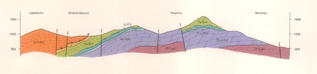
84 82 Alterra-report 2249