Vector Space Modeling for Aggregate and Industry Sectors in Kuwait

Transcription

1 Vector Space Modeling for Aggregate and Industry Sectors in Kuwait Kevin Lawler 1 1 Central Statistical Bureau: State of Kuwait/ U.N.D.P Abstract. Trend growth in total factor productivity (TFP) is unobserved; it evolves continually over time. That assumption is inherent in the use of the Hodrick-Prescott or other bandpass filters to extract trends. Similarly, the Kalman filter/unobserved-components approach assumes that changes in the trend growth rate are normally distributed. In fact, some changes to the trend growth rate of total factor productivity are normally distributed but some may not be, especially in the presence of random technology shocks. The latter distribution may be asymmetric with large outliers. Allowing for those outliers, the estimated trend growth rate changes only infrequently. A strength of the paper is that aggregate trends in TFP are presented, but also industry disaggregated trends estimated by the same techniques. Keywords: Solow Residual, total factor productivity, univariate filters 1 Introduction This argument here records the development of a Kalman Filter and other filters to extract trends in TFP for the Kuwait economy since The Kalman filter was used initially on aggregate trends in Kuwait s GDP. Later the same procedures were used for extracting TFP in Kuwait agricultural, health /education, manufacturing, finance, construction, wholesale and other service sectors. In this way total factor productivity is therefore disaggregated for Kuwait allowing informed policy debate. To begin trend and cyclical components movements in the time series are extractedidentifying key moments and turning points in the time series on economic growth for Kuwait. The relative performance of the Kalman Filter process is then assessed with respect to other filters such as the Hodrick Prescott (HP) procedure. The filters were run against each other for several diverse sectors of the Kuwait economy. The relative performance of the filters are then compared to predicted changes in sector value added as delivered by an estimated Solow growth /Cobb/Douglas production function. Generally all filters performed in roughly uniform terms with regards to directions of change but the Kalman delivers more efficiently on in picking earlier changes in shift factors in trends of TFP. The filters do a broadly similar job in the sector analyses (op. cit.(( Appendices1-3)). The tracking movements for the filters are depicted clearly here. In the future these filters are to be used to develop a composite leading indicator for Kuwait by 922

2 incorporating a Markov procedure to pick early, as distinct from coincident movements in production time series. Agriculture is currently a heavily subsidized sector in Kuwait to engender a strategic shift to national food security. Trends in TFP are therefore vital to monitor so that future agricultural programs can be underpinned with a reliable statistical foundation. All the sectoral analyses indicate generational declines in aggregate and industrial/sector TFP, which are consistent with the literature and other independent studies. In the past high oil prices compensated for this decline in productivity, however, with lower global oil prices Kuwait is likely to move towards enhanced labour intensity based on migrant labour flows from poorer nations in south Asia. The regression analysis in (Appendix 3) demonstrates the significance of TFP on Kuwait growth experience since the This also indicates from that labours share in aggregate production the (Solow coefficient, a) has been increasing since the 1990 s. Given lower real global oil prices, Kuwait may increase its labour intensity profiles in agriculture and other activities. Moreover further analysis of the long-term trends in Kuwait s terms of trade may be an additional factor in stimulating this this process. However, labour productivity fell in the economic crisis of late/early 2008/9, making it more difficult to estimate the trend pace of productivity growth. When the present crisis ends, labour productivity should improve. However this depends in part on the future rate of growth of gross fixed capital formation, and also depends on future growth of total factor productivity (TFP), that is, the Solow residual or technical progress. Several methods for extracting the trend component of total factor productivity are reviewed, to find a procedure that performs efficiently when evaluating trend data and may be used as a guide to the current and possibly future trend in the Kuwait economy s productive potential. A state-space model (Kalman filter Appendix 1) of aggregate/sector output is developed which justifies the use of univariate filters to estimate the trend component of the Solow residual (Appendix 3) The discussion then turns to comment on the use of other linear uni -variate filters available for estimating trends. Appendix (2) depicts relative filters performance in all the sub-sectors investigated for the Kuwait economy since These results demonstrate a solid case for the use of uni-variate filters in agriculture and other sectors since they all track the calculated Solow Residual. (Appendix 3) Of the linear filters, the Kalman filter works best in modeling TFP trends; however, none of the linear filters are fully adequate in modeling total factor productivity. The problem is that innovations creating shocks for trend growth of TFP are not normally distributed; and in particular, significant changes in trend productivity growth appear to occur only at infrequent intervals. The statespace/kalman filter approach instead assumes normally distributed variations to trend growth. Similarly, the Hodrick-Prescott smoothing parameter implicitly assumes a path for trend TFP that is differentiable and whose growth rate evolves continuously. Given estimates of the capital stock, labor quality, and the equilibrium labor share, calculating trend labor productivity amounts to calculating the trend in the Solow residual. This is done following (French, M, W2001) as follows: output (Q) is the product of trend (Q trend ) and gap (Q cycle ). 923

3 Hours supplied (H) is the product of trend hours supplied (H trend ) and a stationary cyclical term (H cycle ). Trend labor (L trend ) is the product of trend hours supplied (H trend ) and the quality of each labor hour (L qual ). A two-factor Cobb-Douglas production function holds in equilibrium. The Solow residual (S) includes cyclical factors as well as trends in total factor productivity (TFP trend ). factor productivity (TFPtrend). *K These five definitions are expressed in equations 1-5: (1) Q = Q trend * Q cycle (2) H = H trend * H cycle (3) L trend = H trend * L qual (4) Q trend = TFP trend * L trend * K 1- (4a) Q = s * ( H * L qual ) * K 1- The observed Solow residual is calculated by inverting equation 4a. Equations 1-4a imply the following relationship between the observed Solow residual and the underlying trend in total factor productivity: (5) S = [Q cycle / H cycle ] * TFP The objective is to extract TFP trend, the unobserved trend in total factor productivity shown in equation 5, from the Solow residual. 2 Methods and Models 2.1 Univariate Methods of Extracting Trend Peak-to-peak interpolation was common in the 1960s (DeLong 1988). From the early to mid-1970s, the deterministic trend was commonly used in describing labor 924

4 productivity or trend output. From 1987 to 1992, several authors began to decompose the sources of trend output growth using aggregate production functions; in essence, the problem shifted from estimating trend labor productivity to estimating trend total factor productivity. In the 1990s and thereafter, trends in output and productivity have frequently been estimated using a stochastic-trend model. The peak-to-peak method has the advantage of simplicity. However, it relies on the questionable assumption that the economy operates at the same level of excess demand at all cyclical peaks. For long expansions, this assumption is harmless, and the procedure works well but for short term movements or, expansions or, periods shortly after downturns, it may be spurious. An Andrews (D, 1993) test for a significant shift in the growth of total factor productivity would indicate a break in average growth, however, a methodology is required that accounts for the possibility of such changes. Three such methodologies are the Hodrick-Prescott (H-P) filter, Christiano s bandpass filter, and trend-cycle decomposition with state-space modeling and the Kalman filter. 2.2 Hodrick-Prescott Filter The Hodrick-Prescott filter estimates trend by smoothing (Appendix 1) in effect, by taking a weighted moving average of the original series, where the moving average is symmetric and centered. In practice, one must choose how smooth the resulting trend should be. In some applications, however, researchers have used a parameters larger values; as the smoothness parameter becomes very large, the H-P filter constructs a linear trend (Cogley,T. 1995).The Hodrick-Prescott filter is quite simple to implement; however, it also has potentially large disadvantages. Unfortunately, the HP filter is optimal only under two fairly restrictive assumptions. First, the data must, a priori, be known to have an I(2) trend. Otherwise, the filter generates shifts in trend growth rates when they are not present in the raw data. If instead there are only one shot permanent shocks to the level of trend, or a constant (split) trend growth rate, or both the H-P filter distorts the cyclical properties and the higher moments of the data in a significant way. If one is not committed to a time-varying trend growth rate, other approaches are preferable to H-P, because they allow for the possibility of a fixed (split) trend growth rate.second, the H-P filter is optimal only if the cycle consists of white noise or, if the identical dynamic mechanism propagates changes in the trend growth rate and in the innovations to the business cycle component. Baxter, (1999) argues both are these conditions are not likely to be co-existing. Moreover, even the best alternatives to the H-P filter are unlikely to be optimal either, as misspecification is a virtual certainty.another weakness of the H-P filter is, that in most published applications, the choice of the smoothness parameter typically has been arbitrary. Uncertainty about an appropriate full-sample smoothing parameter is not the only problem in using the H-P filter. The filter does not possess a reliable method for determining the appropriate gain on new data points at the end of the sample, when the filter is no longer two-sided a marked failure relative to the state-space/kalman filter approach. 925

5 Hamilton argues (1986,), that the Kalman filter is the optimal one-sided filter, with optimal estimate of gain, for any process that linearly links the observed variables with state variables and exogenous and/or lagged dependent variables (i.e. a linear state-space process, with any order of integration). It is optimal among all filters, linear or non-linear, if in addition the state-space model s errors are Gaussian. It is desirable that the distortions created by the H-P filter are small: if they are, its simplicity is a major recommendation. Furthermore, even if the H-P filter is suboptimal, it is not clear that the alternatives are better provided one assumes an I (2) trend a priori. Misspecification problems can make any approach to estimating trend sub-optimal even the two purportedly superior filters, the Bandpass and Kalman filters. 2.3 Kalman filter / State-space Model This approach uses historical data to estimate the share of the variance (of the Solow residual) to assign to trend rather than cycle (Appendix 1). In principle, the approach can also determine whether or not the I (2) component of trend is significantly different from zero a major advantage over the H-P filter. In practice, the state-space/kalman filter approach has an important disadvantage: its variance estimates are biased toward zero when the true variance is small but non-zero. 3 Conclusions None of the linear filters produce a perfect solution.. The H-P and the bandpass filters yield similar results given that the optimal H-P smoothing parameter of, both filters impose I (2) swings on the TFP trend. An awkward remaining problem is to find a structure for modeling trend in total factor productivity that captures random historical shift(s).although linear filters fail to successfully model shifts in trend TFP growth, it may be possible to model such shifts with greater success using an alternative to linear filtering. Hamilton s Markov-switching model (1996, ibid) offers such methodology. Although trend TFP growth declined dramatically in the 2008/9, crisis there is no clear evidence of continuously evolving trend growth in total factor productivity calling into question the usual stochastic trend models or the use of Hodrick-Prescott filtering.how can shifts in trend growth of TFP be extracted more quickly? By utilizing additional information to bear from other supply-side variables, such as labour-force/household - surveys labour cohort analysis and participation rates. But these other supply-side variables feature normal innovations to trend growth whereas shift changes TFP exhibit non-normal innovations. This essay uses data from 1970 to Data for all variables used in the above analysis were taken from data available to the Kuwait (CSB). 926

6 Data on capital [GFCF] is currently being revised with a new methodology, however, quarterly capital stock data produced by CSB which can be interpolated to a quarterly frequency. References 1. Andrews, D.K. (1993), Tests for Parameter Uncertainty and Structural Change with Unknown Change Point, Econometrica, vol. 61, pp Baxter, M. and R. King (1999), Measuring Business Cycles: Approximate Band- Pass Filters for Economic Time Series, Review of Economics and Statistics, vol. 81, pp , November. 3. French,w. (2001)( federal Reserve Washington Reports) 4. Cogley, T. and J. Nason (1995), Effects of the Hodrick-Prescott filter on trend and difference stationary time series: Implications for business cycle research, Journal of 5. Economic Dynamics and Control, vol. 19, pp DeLong, J.B. and L. Summers (1988), How Does Macroeconomic Policy Affect Output, Brookings Papers on Economic Activity 2, pp Hamilton, J. (1986), A Standard Error for the Estimated State Vector of a State- Space Model, Journal of Econometrics, vol. 33, pp

7 Appendix 1 Filter tracking of TFP can be seen in the subsequent graphs along with the Kalman filter specification. The graphs and charts follow the discussion in the text. The CSB macro econometric general equilibrium model was used to estimate value added per sector and in aggregate Initially the macro- economic aggregate picture is shown followed by agriculture and other sectors. The Kalman state space model is given by Y = F T t θ t + v t, v t ~ N(0, V t ) θ t = G t * θ t 1 + w t, w t ~ N(0, W t ) for t = 1,, n. The natrices F t, G t, V t and W t may depend on a parameter vector f. The initialization is given as θ 0 ~ Ν(m 0, C 0 ) a t = G t m t-1 (1) R t = G t C t G T t + W t (2) f t = F T t a t (3) Q t = F T t R t F t + V t (4) e =y f t t t (5) A t = R t F t Q t -1 (6) m t = a t +A t e t (7) C t = R t A t Q t A T t (8) 928

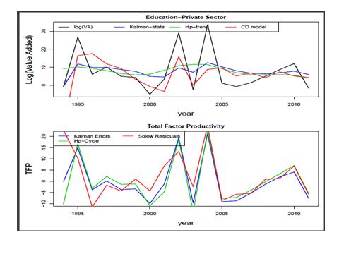
8 Appendix 2. KALMAN Filter Specification/Performance 929

9 930

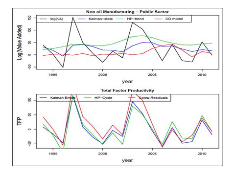
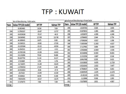
10 Appendix 3. KALMAN Filter Specification/Performance 931

11 932

12 933

13 934

14 935

15 936

16 937