Impact of Global Climate Change and Future Emissions Changes on Regional Ozone and Fine PM 2.5 Levels in North America

Transcription

1 Impact of Global Climate Change and Future Emissions Changes on Regional Ozone and Fine PM 2.5 Levels in North America NARSTO Executive Assembly Meeting Mexico City, Mexico April 8-9, 2008 Praveen Amar NESCAUM (

2 Acknowledgements: K.J. Liao, E. Tagaris, K. Manomaiphiboon, A. G. Russell, School of Civil & Environmental Engineering Georgia Institute of Technology J.-H. Woo, S. He, Emily Savelli, P. Amar Northeast States for Coordinated Air Use Management (NESCAUM) C. Wang Massachusetts Institute of Technology and L.-Y. Leung Pacific Northwest National Laboratory (PNNL) Acknowledgement: US EPA under STAR grant No. R830960

3 Introduction Climate Change is forecast to affect air temperature, humidity, precipitation frequency, etc. Increases in ground-level ozone concentrations are expected in the future due to higher temperatures and more frequent (and longer?) stagnation events ( climate change penalty ); effect on PM 2.5 levels less certain. Accurate projections of emissions of ozone and PM 2.5 precursors to distant future (year 2050) are key to evaluate the relative impacts of climate change and current control strategies on ambient levels of ozone and PM 2.5 The effects (direct and indirect) of ground-level air pollution on climate (regional and global) are not investigated here.

4 Issues How does the climate change penalty compare to benefits of planned emission reductions? How well will currently planned control strategies work as changes in climate occur? How robust are the results? Above questions can be answered by quantifying sensitivities of air pollutants (e.g., ozone and PM2.5) to their precursor emissions (e.g., NOx, NH3, biogenic and anthropogenic VOCs and SO2) and associated uncertainties.

5 Modeling Procedure Leung and Gustafson (2005) NASA GISS IPCC A1B MM5 MCIP With 2050 climate With 2001 & 2050 climate SMOKE (w/ 2001 EI) SMOKE (w/ 2050 EI) CMAQ-DDM *Leung and Gustafson (2005), Geophys. Res. Lett., 32, L16711

6 147 x 111 grid cells 36-km by 36-km grid size 9 vertical layers 5 U.S. sub-regions 2 Canadian sub-regions Northern Mexico

7 Emission Inventory Projection Accurate projection of emissions is key to comparing relative impacts on future air quality and for evaluating control strategy effectiveness Academic and Policy/Government: Cooperative Effort Woo et. al, 2006

8 Projecting emissions - US - Step #1: Obtain national projection data available for the near future - Use EPA CAIR Modeling EI (Point/Area/Nonroad, from Y2001 to Y2020) - Use RPO SIP Modeling EI (Mobile, from Y2002 to Y2018) Step #2: Obtain growth data for the distant future and develop crossreference - Use IMAGE model (IPCC SRES, A1B) - From Y2020 (Y2018 for mobile activity) to Y X-Ref : Sectors/Fuels combination to SCCs Step #3: Apply growth factors using cross-reference - Use IMAGE model (IPCC SRES, A1B) - From Y2020(Y2018 for mobile activity) to Y2050

9 Projecting emissions - CANADA/MEXICO - Step #1: Obtain national projection data available for the near future or update base year inventory - Use Y2020 Environmental Canada Future EI (Area/Mobile) - Use Y2002 Point source inventory (NYS DEC) scaled with Y2000 by-state point source summary from Environment Canada - Update base year Mexico inventory using Mexico NEI for 6 US-Mexico Border states Step #2: Obtain simple growth data for the distant future - Use IMAGE model (IPCC SRES, A1B) - From Y2020 to Y2050 (CAN, Area/Mobile) - From Y2002 to Y2050 (CAN, Point) - From Y1999 to Y2050 (MEX, All)

10 Comparison of existing future-ei development approaches Name Base Year Future Years Geographical Domain Scenario Source sectors Chemical species Model Availabili ty EPA CAIR /2015 /2020 Continental US EPA BASE /CAIR EGUs, non-egus NOx, VOCs, CO, NH3, SO2, PM IPM /EGAS/NMI M Yes EPA CSI /2020 Continental US EPA BASE /CSI EGUs, Non-EGUs NOx, VOCs, CO, NH3, SO2, PM IPM /EGAS Yes RPOs /2018 Continental US OTB/OTW EGUs & non-egus NOx, VOCs, CO, NH3, SO2, PM IPM /EGAS Partly SAMI (/10yrs) 38 States + DC OTB/OTW/BW C/BB EGUs & non-egus NOx, VOCs, CO, NH3, SO2, PM SAMI No RIVM* 1995 ~2100 (/yr) World (17 regions) IPCC SRES(A1, B1, A2, B2) Energy sector/fuel combination CO2, CH4, N2O, CO, NOx, SO2, NMVOC IMAGE Yes NESCAUM /EPA 1999 ~2029+ (/3yrs) Units(EGUs), States(NE), Country BAU, RGGI Energy sector/fuel combination NOx, VOCs, CO, NH3, SO2, PM MARKAL 2007 Pros Cons Both RIVM : Netherlands s National Institute for Public Health and the Environment IMAGE : Integrated Model to Assess the Global Environment

11 RIVM IMAGE IMAGE: A dynamic integrated assessment modeling framework for global change WorldScan (economy model), and PHOENIX (population model) feed the basic information on economic and demographic developments for 17 world regions into three linked subsystems (EIS, TES, and AOS*) *EIS(Energy-Industry System), TES(Terrestrial Environment System), AOS (Atmospheric Ocean System)

12 Linking the Two Futures: CAIR and IMAGE Calculate combined factor of growth/control from EPA base year(2001) vs. future year (2020) emissions inventory Calculate growth factor for Y Y2050 (A1B) from IMAGE Calculate growth factor for Y2001 -Y2050 for Canada/Mexico from IMAGE RPO 2018 Activity data (On-road mobile) Use EPA 2020 CAIR-case inventory Compare EPA CAIR vs. IMAGE for Y2001 -Y2020 Develop SCC to IMAGE fuel/sector x -reference Update cross-references Check/apply growth factors to 2020 EPA CAIR EI to get 2050 EI SMOKE/M6- ready activity data for 2050

13

14 Regional Emissions: Projections Year 2001 Year Millions TPY Year Pnt Area Nonroad Onroad Present and future years NOx emissions by state and by source types

15 Spatial Distribution of US Emissions (NMVOC) Millions TPY Pnt Area Nonroad Onroad 2050

16 Future Emissions (CANADA) Millions TPY Millions TPY CO NOX VOC NH3 SO2 PM10 PM2_5 CAN00_Pt CAN00_Ar CAN00_Nr CAN00_Mb CO NOX VOC NH3 SO2 PM10 PM2_5 CAN50_Pt CAN50_Ar CAN50_Nr CAN50_Mb

17 Future Emissions (Mexico) Millions TPY Millions TPY CO NOX VOC NH3 SO2 PM10 PM2_5 Mex1999_Pt Mex1999_Ar CO NOX VOC NH3 SO2 PM10 PM2_5 MEX2050_Pt MEX2050_Ar

18 Emissions Projections (Three Countries) _np 60 Emissions (million tons per year) NOX VOC PM25 SO2 NH : NOx: -50% VOC s: +2% PM2.5: -10% SO2: -50% NH3: +7% 2050np 2001: VOC s: +15% np (non-projected): Emission Inventory 2001, Climate 2050

19 Summary of Air Quality Simulations Scenario Emission Inventory (E.I.) Climate Conditions Future Air Quality Impacting Factors 2001 Historic (2001) Historic (2001 whole year) N.A summers Historic ( ) Historic ( summers) N.A. 2050_np (nonprojected emissions, but meteorologically influenced for consistency) Historic (2001) Future (2050 whole year) Potential future climate changes _np summers Historic ( ) Future ( summers) Potential future climate changes 2050 Future (2050) Future (2050 whole year) Potential future climate changes & projected E.I summers Future ( ) Future ( summers) Potential future climate changes & projected E.I.

20 Assessment: Part I Impact of Future Climate Change Alone on Ground-level Ozone and PM 2.5 Concentrations important and interesting for comparison with the case with emission controls

21 Daily maximum 8 hour ozone concentration CDF plots in 2001, 2050 and 2050_np CDF NOx limitation sharpening S, reducing peak Southeast Reduced NOx scavenging M8hO 3 (ppb) _np Small increase in O3 due to climate Substantial decrease in O3 due to planned emission controls CDF US M8hO 3 (ppb) Peaks (ppb) 2001: 141 (actual= 146) 2050_NP: : _np

22 Daily maximum 8 hour ozone concentration CDF plots in 2001, 2050 and 2050_np CDF Northeast M8hO 3 (ppb) _np CDF US M8hO 3 (ppb) _np Peaks (ppb) 2001: 141 (actual= 146) 2050_NP: : 120

23 Summer Average Max 8hr O 3 O3_ summers O3_ summers O3_FutureSummers - O3_HistoricSummers O3_FutureSummers - O3_FutureSummers_np np: Emission Inventory 2001, Climate 2050

24 PM2.5_2001 Annual PM 2.5 PM2.5_2050 PM2.5_ PM2.5_2001 PM2.5_ PM2.5_2050np np: Emission Inventory 2001, Climate 2050

25 Impact of Potential Climate Change and Planned Controls on Average Max8hrO3 All grid averages (not just monitor locations) ( Max8hrO3 (ppbv) _np Summers Summers Summers _np _np Summers Summers Summers _np West Plains Midwest Northeast Southeast US ppbv lower in 2050 (6-15%) -About +/- 1ppbV difference without considering future emission controls (2050_np) (-2 to + 3%) - More significant reductions in summers. (12-28%)

26 Impact of Potential Climate Change on PM 2.5 ( PM2.5 (_g/m3) _np Summers Summers Summers _np West Plains Midwest Northeast Southeast US - about µg/m 3 lower in maximum 0.6 µg/m 3 difference without considering future emission controls (2050_np) -Usually np is lower in summer, though can be higher on average

27 Annual Averaged Changes from 2001 in Averaged Max8hrO3 & PM 2.5 Max8hrO3 (%) PM 2.5 (%) np np West Plains Midwest Northeast Southeas t US

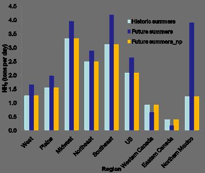
28 M8hO 3 (%) Summers Summers_np West Plains Midwest Northeast Southeast US Western Canada Eastern Canada Northern Mexico PM 2.5 (%) Summers Summers_np West Plains Midwest Northeast Southeast US Western Canada Eastern Canada Northern Mexico

29 Regional Predicted Max8hrO3 Characteristics Unit of 99.5% and peak: ppbv summers # of days over 80 ppb # of days over 85 ppb (sim/act) Peak summers # of days over 80 ppb # of days over 85 ppb Peak # of days over 80 ppb _np summers # of days over 85 ppb Peak West / Los Angeles / Plains / Houston / Midwest / Chicago 78 66/ Northeast / New York 51 38/ Southeast / Atlanta /54* 124/ Significant improvement Stagnation events Increase in some areas * : 137

30 Assessment: Part II Sensitivity Analysis of Ground-level Ozone and PM 2.5 Now this is more of our focus

31 Semi normalized First-order Sensitivity Calculated using DDM-3D S S i, j i, j = E Si,j : sensitivity j! C! E Ci : concentration of pollutant i Ej : emission of precursor j i j Sensitivities are calculated mathematically (about 12 per run) and have the same units as concentration of the air pollutants. Local sensitivity Relative response to an incremental change in emissions Read results as the linearized response to a 100% change C C o C p p + E p Δ E o + E o C E

32 Sensitivities of Daily 4 th Highest 8-hr Ozone Sensitivity (ppbv) Ozone to anthropogenic VOCs * _np _Norm _summers _np_summers _summers Sensitivity (ppbv) Sensitivity (ppbv) West Plains Midwest Northeast Southeast US O Ozone to biogenic VOCs * 2 3 precursor sensitivities to NOx enhanced (ppb/ton) due to both controls (primary) and climate from 2001, VOC sensitivities increased from climate, decreased due to controls West Plains Midwest Northeast Southeast US Ozone to anthropogenic NO x West Plains Midwest Northeast Southeast US Norm: Adjusted for emissions change

33 Spatial Distribution of Sensitivities of Annual Ozone to Anthropogenic NO x Emissions _np _Norm

34 Sensitivity(ug/m^3) Sensitivities of Speciated PM 2.5 Formation PM 2.5 precursor sensitivities (µg m -3 per ton) similar to 2001 Northeast Sensitivity(ug/m^3) ASO4_SO2 ASO4_NH3 ASO4_NOX_A ANO3_NOX_A US ANO3_NH3 ANO3_SO2 ANH4_NH3 AORGB_VOC_B

35 Spatial Distribution of Sensitivities of PM 2.5 Formation to SO 2 Emissions _np _N

36 Assessment: Part III Uncertainty Analysis of Impact of Climate Change Forecasts on Regional Air Quality and Emission Control Responses A second central question

37 Summary of Uncertainty Simulations Scenario High-Extreme Scenario Base Scenario Low-Extreme Scenario Perturbations 99.5 % percentile of 3-D temperature and absolute humidity 50.0 % percentile of 3-D temperature and absolute humidity 0.5 % percentile of 3-D temperature and absolute humidity Sources IGSM and GISS IGSM ~IPCC A1B scenario IGSM and GISS Tried here first

38 CDFs of Max8hrO3 and 24-hr PM 2.5 in Summer of shown for comparison Fractile Max8hrO3 (ppbv) Peaks (ppb) 2050_99.5: _50: _0.5: 126 Fractile Low_extreme Base High-extreme hr PM 2.5 (ug/m^3)

39 No. of Days M8hrO3 > 80ppbV in Summer of 2050 Region / City Low-extreme (0.5%) Base (50%) High-extreme (99.5%) West / Los Angeles 2 Days 6 Days 7 Days Plains / Houston 5 Days 10 Days 24 Days Midwest / Chicago 3 Days 4 Days 6 Days Northeast / New York Southeast / Atlanta Days

40 Temperature Uncertainties low base high low - base high - base

41 PM 2.5 Uncertainties low base high low - base high - base

42 Uncertainties in Summertime Max8hrO3 and PM 2.5 Max8hrO3 PM 2.5 (High-extreme scenario) (Base scenario)

43 Uncertainty in PM 2.5 Sensitivity Sensitivity (!g/m^3) Sensitivity (!g/m^3) Sensitivity (!g/m^3) PM 2.5 to SO 2 Low-extreme Base High-extreme West Plains Midwest Northeast Southeast US PM 2.5 to anthropogenic NO x PM 2.5 precursor sensitivities relatively unchanged West Plains Midwest Northeast Southeast US PM 2.5 to NH 3 West Plains Midwest Northeast Southeast US

44 How do uncertainties in climate change, impact the ozone and PM 2.5 concentrations and sensitivities? Results suggest that modeled control strategy effectiveness is not affected significantly, however, areas at or near the NAAQS in the future should be concerned about the impact of uncertainty of future climate change.

45 Conclusions Climate change, alone, with no emissions growth or controls, has mixed effects on the ozone and PM 2.5 levels as well as on their sensitivities to precursor emissions. Ozone generally up ( climate change penalty ), PM mixed The impact of changes in precursor emissions due to planned controls and anticipated changes in activity levels on the ozone and PM 2.5 levels is higher than the impact of climate change alone on ozone and PM 2.5 levels. Carefully forecasting emissions is critical to relevancy of results Spatial distribution and annual variations in the contribution of precursors to ozone and PM 2.5 formation remain quite similar. Sensitivities of ozone to NOx increase on a per-ton basis, mostly due to reduced NOx levels, and a bit due to climate change Sensitivities of PM 2.5 to precursors similar on per ton basis Lower NOx and higher NH 3 emissions increase sensitivity of NO3 to NOx in 2050 projected emissions case

46 Conclusions (cont d) Controls of NO x and SO 2 emissions will continue to be effective The uncertainties in future climate change have a relatively modest impact on simulated future ozone and PM 2.5 Extremes simulated to get significant changes High-extreme (99.5 th percentile) led to increases in ozone and PM. Addressing uncertainties suggests that control choices are robust

47

48 Keeling Curve (11,000 feet, Mauna Loa, Hawaii): Very Predictable CO 2 Levels under Business-as- Usual Practices: 316 ppm in 1959, 379 ppm in 2005, 500 ppm expected in mid-century (exceeds by far the natural range over the last 650,000 years ( 180 to 300 ppm)

49 Additional Slides

50 ΔP:

51 PM 2.5 composition (%) SO 4 (%) NO 3 (%) NH 4 (%) OC (%) EC (%) OTHER (%) Historic summers West Plains Midwest Northeast Southeast US Western Canada Eastern Canada Northern Mexico Future summers_np West Plains Midwest Northeast Southeast US Western Canada Eastern Canada Northern Mexico

52 Historic summers PM 2.5 composition (%) SO 4 (%) NO 3 (%) NH 4 (%) OC (%) EC (%) OTHER (%) West Plains Midwest Northeast Southeast US Western Canada Eastern Canada Northern Mexico Future summers West Plains Midwest Northeast Southeast US Western Canada Eastern Canada Northern Mexico

53 Method Step 2: Estimate uncertainties GISS GCM IGSM GCM MM5 Remapping Temperature and Humidity INDERMIDIATE METEOROLOGY MM5 MCIP 99.5 th percentile (High) 50 th percentile (Base) 0.5 th percentile (Low) EI SMOKE CMAQ

54 Uncertainty Simulations Our studies suggested that T and Abs. Hum. had major impacts Perturbations: -- 3-dimensional temperature -- 3-dimensional absolute humidity Tried here first Levels of perturbation: th percentile (High-extreme) th percentile (Base: rerun *) th percentile (Low-extreme) *For consistency, the 50 th percentile is rerun as the fields are changed since the IGSM monthly average distribution is not identical to the GISS-MM5

55 Uncertainties in Meteorology Temperature 2001_summer 2050_summer 99.5 th percentile (High-extreme) Temperature (K) West Plains Midwest Northeast Southeast US 50 th percentile (Base scenario) 0.5 th percentile (Low-extreme) Absolute Humidity (Kg/Kg) 2.0E E E E-03 Abs. Humidity 2001_summer 2050_summer 0.0E+00 West Plains Midwest Northeast Southeast US