Measuring Environmental Justice to Create Sustainable Regions

Transcription

1 Measuring Environmental Justice to Create Sustainable Regions Feb. 27, 2015 Madeline Wander, Data Analyst, USC PERE OVERVIEW OF TODAY S WORKSHOP GOALS: To introduce the use of public data for equity analyses, using the Environmental Justice Screening Method as an example To explore ways to use equity analyses in your own work AGENDA: 1. Round of introductions 2. Overview of USC PERE and our work 3. Presentation on EJ and the EJSM *Please ask questions along the way! 4. Small group exercise 5. Report backs Source: February

2 USC PROGRAM FOR ENVIRONMENTAL & REGIONAL EQUITY (PERE) Our mission is to conduct research and facilitate discussions on issues of environmental justice, regional equity, and social movement building. Our work is rooted in the three R s: Reach Relevance Rigor February WHAT IS USC PERE? We seek direct collaborations with community-based organizations in research and other activities, trying to forge a new model of how university and community can work together for the common good. February

3 OUR FRAME Conventional wisdom in economics says there is a trade-off between equity and efficiency. But, new evidence suggests that regions that work toward equity have stronger and more resilient economic growth as well as environmental sustainability for everyone. February PERE S EJ WORK PERE s work on environmental justice includes: Determining localized impact and broader patterns of environmental inequality by analyzing government databases Collaborating with community organizations to check the data against the facts on the ground and make policy recommendations Convening community organizers, researchers, government agencies, and funders to advance the field together February

4 ENVIRONMENTAL JUSTICE 101 WHAT IS ENVIRONMENTAL JUSTICE? Environmental justice (EJ) is rooted in the belief that all people regardless of race, ethnicity, gender, or income have the right to a clean and healthy environment in which to live, work, go to school, play, and pray. EJ ensures: 1. Equitable distribution of environmental burdens and benefits 2. Fair and meaningful participation in decision-making processes February

5 WHAT IS ENVIRONMENTAL JUSTICE? EJ efforts originally focused on uneven siting of hazardous industrial development but today s efforts span multiple and diverse areas and geographies. EJ is about providing benefits to communities as well as reducing burdens. February HISTORY OF ENVIRONMENTAL JUSTICE EJ has its roots in environmental and civil rights movements 1980s: Rise of the Environmental Justice movement 1983: Solid Waste Sites and the Black Houston Community by Robert Bullard 1987: Toxic Wastes and Race in the United States by the United Church of Christ Commission on Racial Justice February

6 WHAT HAS RESEARCH SHOWN? Two main findings: 1. Disparities in exposures to environmental hazards between racial and socioeconomic groups are significant and are linked to adverse health risks 2. Patterns of inequality are not just attributable to income or land use race matters, too Manuel Pastor, Rachel Morello-Frosch and James Sadd, Still Toxic After All These Years: Air Quality and Environmental Justice in the San Francisco Bay Area (Santa Cruz, CA: Center for Justice, Tolerance and Community, University of California, Santa Cruz, 2007). February EJ CAN HELP ACHIEVE SUSTAINABILITY FOR ALL In regions with higher disparities in exposure rates between whites and people of color, exposure rates are higher for everyone. Average exposure by race/ethnicity in Metros with low, medium and high minority discrepancy scores Source: Michael Ash et al., Is Environmental Justice Good for White Folks? (Amherst, MA: University of Massachusetts, Amherst, Department of Economics, Working Paper , July 2010). February

7 ADDRESSING EJ THROUGH MEASURING We can only make progress on what we can measure but how do you measure environmental justice? To do this, we created the Environmental Justice Screening Method, which uses a Cumulative Impact approach examine multiple environmental and social stressors and links to environmental health disparities. Traditional risk assessment does not account for the combination and potential interaction of hazard exposures and socioeconomic stressors. Science needs to catch up to community wisdom. Principle Investigators: Rachel Morello-Frosch (UC Berkeley), Manuel Pastor (USC), and Jim Sadd (Occidental College) February EJSM OVERVIEW 7

8 ENVIRONMENTAL JUSTICE SCREENING METHOD (EJSM) The goal is to develop indicators of cumulative impact that: Reflect current research on environmental and social determinants of health Are transparent and relevant to policy-makers, regulators, and communities The applications include: Land use planning Funding allocations Regulatory decision-making and enforcement Community outreach and engagement February EJSM OVERVIEW Maps where people are exposed Measures the cumulative impact of a variety of factors All underlying data is public: most comes from U.S. Census, U.S. EPA, and CalEPA All mapping done at the Census tract level Scoring system based on rankings: each tract receives points related to indicators Statewide coverage, REGIONAL scoring February

9 WHY REGIONS? The regional scale is key: Each region has its own set of industries and pollution problems Transportation and land use issues are regional in scale Disparities often wash-out at the national or even state levels but are apparent at the regional level February EJSM OVERVIEW 4 Categories of Indicators The Cumulative Impact Proximity to Hazards and Land Uses Associated with Air Pollution, and Sensitive Land Uses Health Risk and Exposure Indicators Social and Health Vulnerability Indicators Climate Change Vulnerability Indicators February

10 EJSM OVERVIEW Cumulative Impact (CI) Score = Hazard Proximity and Sensitive Land Use Score (1-5) + Health Risk and Exposure Score (1-5) + Social and Health Vulnerability Score (1-5) + Climate Change Vulnerability Score (1-5) February EJSM ARCHITECTURE STEP 1: GIS Spatial Assessment (create CI poly layer [residential and sensitive land uses] with Census block info and calculate hazard proximity metrics) STEP 2: SPSS Programming (data processing and generation of CI scores for tracts) STEP 3: GIS Mapping of CI scores February

11 EJSM DEVELOPMENT EJSM was contracted by CA Air Resources Board and co-created with stakeholder input (scientific review committee, regulatory scientists from different agencies, decision-makers, and community organizations): Helped identify indicators and priorities Participated in an iterative process of review and methodological improvements Engaged in ground-truthing interim results and government databases February EJSM LAYER 1 Proximity to Hazards & Sensitive Land Uses 11

12 LAYER 1 HAZARD PROXIMITY INDICATORS Facilities reporting Greenhouse Gas emissions and toxic air pollution (about 3,000 facilities) Greenhouse Gas (GHG) Mandatory Reporting database under AB 32 CA Emission Inventory Development and Reporting Systems (CEIDARS) Industry-wide layers Hazardous land uses Sensitive land uses Auto paint and body shops Gas stations Permitted hazardous waste sites Rail Ports Airports Refineries Intermodal distribution facilities Traffic volume Childcare facilities Hospitals Senior housing Schools Playgrounds and parks February GROUNDTRUTHING THE DATA LOCATION CORRECTION of Facilities of Interest in the San Joaquin Valley FOI facility location as reported by CARB Corrected location February

13 LAYER 1 HAZARD PROXIMITY METHODS ORIGINAL BUFFER TOOL for identifying hazard proximity Each CI poly receives a hazard proximity score, with the number of hazards weighted using distance ( wedding cake approach ). Distance Band Weight Hazard Count 1,000 ft ,000 ft ,000 ft Distance-weighted hazard score = ( 1.0 x 2 ) + ( 0.5 x 8 ) + ( 0.1 x 6 ) 1,000 ft. band 2,000 ft. band 3,000 ft. band February LAYER 1 HAZARD PROXIMITY METHODS NEW POINT DISTANCE TOOL for identifying hazard proximity The Point Distance Tool measures the distance between the CI poly centroids and point hazards within a specified threshold. The tool generates a table specifying the distance between the CI poly centroid and the point hazard. CI Poly Centroid ID Hazard ID Distance 101 A B C 1700 NOTE: We only show the relationship between the CI Poly centroid and three hazards for sake of simplicity. February

14 LAYER 1 HAZARD PROXIMITY METHODS NEW POINT DISTANCE TOOL for identifying hazard proximity How do we calculate the Hazard Proximity Scores for each CI Poly? First sum the hazards that fall within 1000, 2000, and 3000 feet of each CI poly centroid CI Poly Centroid ID Hazard ID Distance 101 A B C 1700 CI Poly Centroid ID Hazard Count ft Hazard Count ft Hazard Count ft B+C A As with the Buffer Tool, the hazard count is weighted according to buffer distance. February LAYER 1 HAZARD PROXIMITY METHODS NEW POINT DISTANCE METHOD for identifying hazard proximity This method works best with small, equant polygons 1000 ft Buffer Large, oddly shaped polygons require additional processing 1000 ft 1000 ft 1000 ft Buffer February

15 LAYER 1 HAZARD PROXIMITY METHODS NEW POINT DISTANCE METHOD for identifying hazard proximity Solution: Cut large CI polys using a grid and run Point Distance for each centroid 1000 ft 1000 ft 1000 ft February LAYER 1 HAZARD PROXIMITY METHODS Wait! Don t we need to account for the area of the CI poly when identifying nearby hazards? The Point Distance Tool measures the distance between two points, rather than the distance between a point and a polygon (like the Buffer Tool does). 3,000 ft. Buffer Tool: CI Poly Hazard 3,000 ft. Point Distance Tool: CI Poly Centroid same distance doesn t capture the same area. Hazard February

16 LAYER 1 HAZARD PROXIMITY METHODS To address this problem, we add the radius of a circle with the equivalent area to the CI poly to each of the distance bands in our SPSS programming. This way, we can identify how many hazards are within 1000, 2000, and 3000 feet of a CI poly. 3,000 ft. Gap! CI Poly Centroid Hazard Radius + 3,000 ft. CI Poly Centroid + Radius Hazard February LAYER 1 HAZARD PROXIMITY METHODS RECALL: The Point Distance tool in ArcGIS measures the distance between each CI poly and nearby hazards. Within the Point Distance output, each row lists the distance between a CI poly and a hazard -- or, a unique CI polyhazard relationship. Our SPSS program aggregates these outputs to summarize the total number of hazards by type falling within three distance buffers around each CI poly. Notice that you can change the distance buffers simply by typing new values here! February

17 LAYER 1 HAZARD PROXIMITY METHODS Final step: aggregating hazard counts to block to tract using population weights (in SPSS) Hazard Proximity Counts for each block calculated in same way as Buffer Method Tract Percent of tract population that lives in each block Hazard Proximity Score for tract 4 5 X 40% 10% = % 2 Block 20% Hazard Proximity Score for tract = (4 x.40) + (5 x.10) + (2 x.20) + (4 x.30) = 4 February

18 EJSM LAYER 2 Health Risk & Exposure LAYER 2 HEALTH RISK & EXPOSURE INDICATORS RSEI (Risk Screening Environmental Indicators), average toxic concentration hazard scores PM 2.5 interpolated annual average concentration, Ozone concentration, NATA (National Air Toxics Assessment) respiratory hazard from mobile and stationary sources, 2005 NATA inhalation cancer risk, 2005 Pesticide applications, February

19 EJSM LAYER 3 Social & Health Vulnerability 19

20 LAYER 3 SOCIAL & HEALTH VULNERABILITY Socioeconomic vulnerability Biological vulnerability Political vulnerability % residents of color % residents below twice national poverty level % renter Median housing value % population >24 with less than a high school education % <5 years old and % >60 years old % pre-term of SGA infants, % >4 in HH where no one >15 speaks English well % votes cast among all registered voters averaged for 2004, 2006, 2008, 2010 general elections mostly from American Community Survey data February

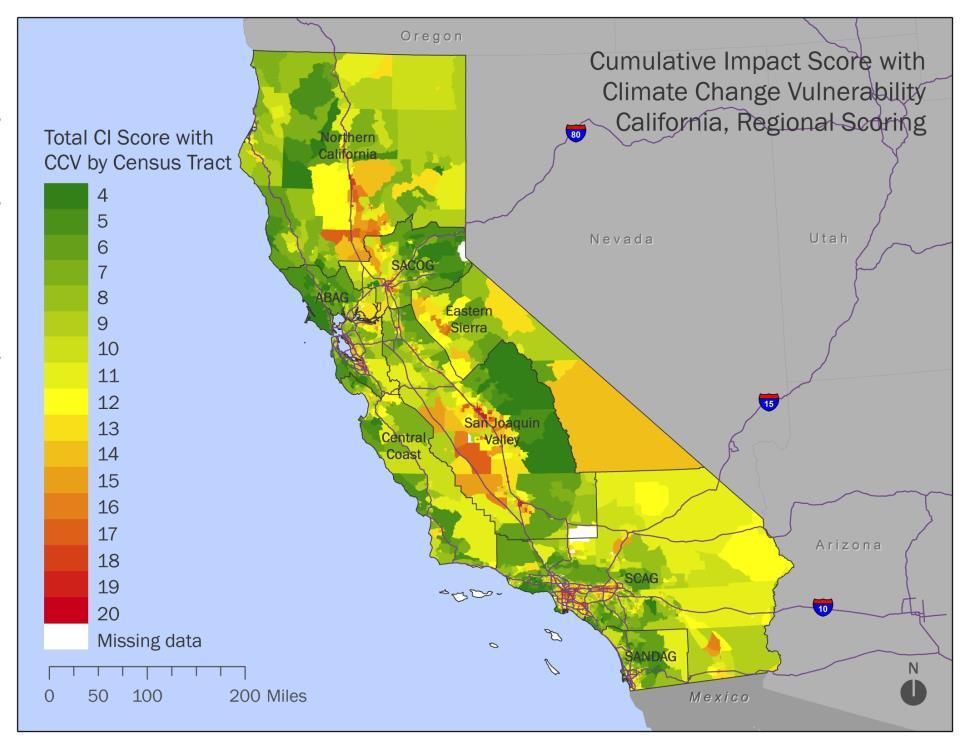
21 EJSM LAYER 4 Climate Change Vulnerability LAYER 4 CLIMATE CHANGE VULNERABILITY INDICATORS Heat Island Risk Temperature Mobility / social isolation % tree canopy % impervious surface Projected max monthly temperature Change in projected max monthly temperature Change in degree-days of warm nights % elderly living alone % car ownership National Land Cover Data, 2001 National Center for Atmospheric Research, downscaled Community Climate System Model, scenario B1, ensemble average & Cal ADAPT American Community Survey (ACS), USC PERE February

22 CUMULATIVE IMPACT SCORE 22

23 CUMULATIVE IMPACT SCORE Cumulative Impact Score = Hazard Proximity and Sensitive Land Use Score (1-5) + Health Risk and Exposure Score (1-5) + Social and Health Vulnerability Score (1-5) + Climate Change Vulnerability Score (1-5) February

24 24

25 APPLICATIONS OF EJSM 25

26 COMMUNITIES USING EQUITY ANALYSES Example: Clean Up, Green UP campaign in Los Angeles Campaign aims to provide special assistance to prevent new siting while also helping businesses convert to safer, cleaner processes EJSM helped identify environmentally overburdened and socially vulnerable communities Researchers have also trained and collaborated with community on data gathering, analysis, and presentation Source: Elva Yañez February AGENCIES USING EQUITY ANALYSES Explore CalEnviroScreen 2.0 HERE February

27 FOR MORE, CHECK OUT OUR WEBSITE QUESTIONS? February SMALL GROUP EXERCISE 27

28 SMALL GROUP EXERCISE Form a group of 5 or 6 people focused on a social justice issue. In your group, work through the following questions: 1. Name the problem. What is a research question that would help measure, and so address, this problem? 2. What data would help answer this question? Do you know of any public databases that contain these data? Who is the impacted community and are there mutually-beneficial opportunities for them to get involved in this step? 3. Who are the audiences like government agencies or community organizations that would be interested in your exploration of this question? Be specific. 4. What are the planning, policy, or budgeting implications of exploring this research question? What are the organizing implications? February