Matt Sloat, Gordon Reeves, Kelly Christiansen

Transcription

1 Predicting the response of salmon habitat to changing hydrologic regimes in southeast Alaska Matt Sloat, Gordon Reeves, Kelly Christiansen Wild Salmon Center USFSPNW Research Station

2 Funding provided by: Additional assistance provided by: TNF, UCSB Marine Science Institute, UC Davis, Oregon State University, and USFS PNW RS.

3 Objectives: Determine the vulnerability of southeast Alaska watersheds to potential impacts of climate change. Focus on changes in flood disturbance in response to trends for a warmer, wetter climate. Determine the impact of increases in mean annual flooding on spawning habitat for Pacific salmon.

4 Pacific salmon prefer to spawn in particular geomorphic settings High quality: small to large floodplain reaches Paustian et al Moderate quality: moderate gradient, small to large confined reaches

5 Pacific salmon prefer to spawn in particular geomorphic settings High quality: medium to large estuarine and floodplain reaches High quality: small estuarine reaches Paustian et al Moderate quality: moderate gradient, medium to large confined reaches

6 Pacific salmon prefer to spawn in particular geomorphic settings High quality: medium to large estuarine and floodplain reaches High quality: small estuarine reaches Paustian et al Moderate quality: moderate gradient, medium to large confined reaches

7 Where do these habitats occur on the landscape? What is their exposure to climate-induced hydrologic change? What is their sensitivity to hydrologic change?

8 Where do these habitats occur on the landscape? Use synthetic stream network generated from 20m DEM (Netmap). Parameterize stream reaches (e.g., width, depth, substrate size) using field measurements and numerical models.

9 Netmap stream network >800 HUC 12 watersheds. No transboundary watersheds, primarily non-glacial.

10 >800 HUC 12 watersheds. No transboundary watersheds, primarily non-glacial.

11 DEM-derived channel slope

12 w = A ; R 2 = 0.92 Bank-full channel depth (h bf ) h = A ; R 2 = 0.71 Zynda, T. (2005) Unpublished Master s Thesis, Michigan State University, Lansing MI. Wood-Smith RD, Buffington JM (1996) Earth Surface Processes and Landforms, 21,

13 Spatially explicit prediction of median gravel size is used to assess the extent of reaches with suitable size gravel for salmon spawning Substrate Size Models Buffington et al. (2004) CJFAS, 61, D 50 range mm Surface substrate size characterized by median grain size (D 50 ) and predicted by : D 50 = (ρhs) 1-n /(ρ s -ρ)kg n

14 Gravel Scour Potential Models Haschenburger (1999) Water Resources Research,35, Probability of egg mortality from scour < 50% > 50% Goode et al. (2013) Hydrologic Processes, 27,

15 What is their exposure to climate-induced hydrologic change? Regional hydrologic model (Curran et al. 2003) to predict current and future mean annual flood size (a.k.a., bankfull flood, Q 2, 50% flood).

16 Why focus on mean annual floods? Given enough time, rivers construct their own channels. A river channel is characterized in terms of its bank-full geometry. Bank-full geometry is defined in terms of river width and average depth at bank-full discharge. Bank-full discharge (~Q 2 ) is the flow discharge when the river is just about to spill onto its floodplain. Floods with this recurrence interval should have a pervasive influence on salmon populations, as opposed to less frequent, higher magnitude floods that may only impact individual cohorts.

17 A warmer, wetter future for SE AK will produce larger mean annual floods (Q 2 ) Percent increase Percent increase

18 A warmer, wetter future for SE AK will produce larger mean annual floods 100 Predicted increase in southeast AK flood magnitude Median: 18% 28% Number of watersheds Percent increase in mean annual flood magnitude

19 What is their sensitivity to hydrologic change? Substrate change (D50, scour) sensitive to changes in flow depth, not necessarily discharge. Need to understand reach scale variation in discharge-flow depth relationships.

20

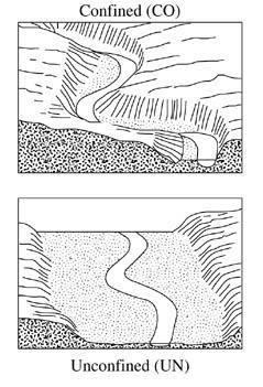
21 Depth (h) Static channel morphology Unconfined channels New h h bf Q 2 New Q 2 Flood magnitude (Q)

22 Depth (h) Static channel morphology Confined channels New h h bf Q 2 New Q 2 Flood magnitude (Q)

23 What is their sensitivity to hydrologic change? Channels may change in multiple dimensions.

24 Depth (h) Dynamic channel morphology Unconfined channels h bf Q 2 Flood magnitude (Q)

25 Depth (h) Dynamic channel morphology Unconfined channels New h bf New Q 2 Flood magnitude (Q)

26 Depth (h) Dynamic channel morphology Confined channels h bf Q 2 Flood magnitude (Q)

27 Depth (h) Dynamic channel morphology Confined channels New h bf New Q 2 Flood magnitude (Q)

28 Scenarios Static Dynamic Change in flow depth (h): Confined: h now << h future Unconfined: h now = h future Change in flow depth (h): Confined: h now < h future Unconfined: h now < h future

29

30

31

32

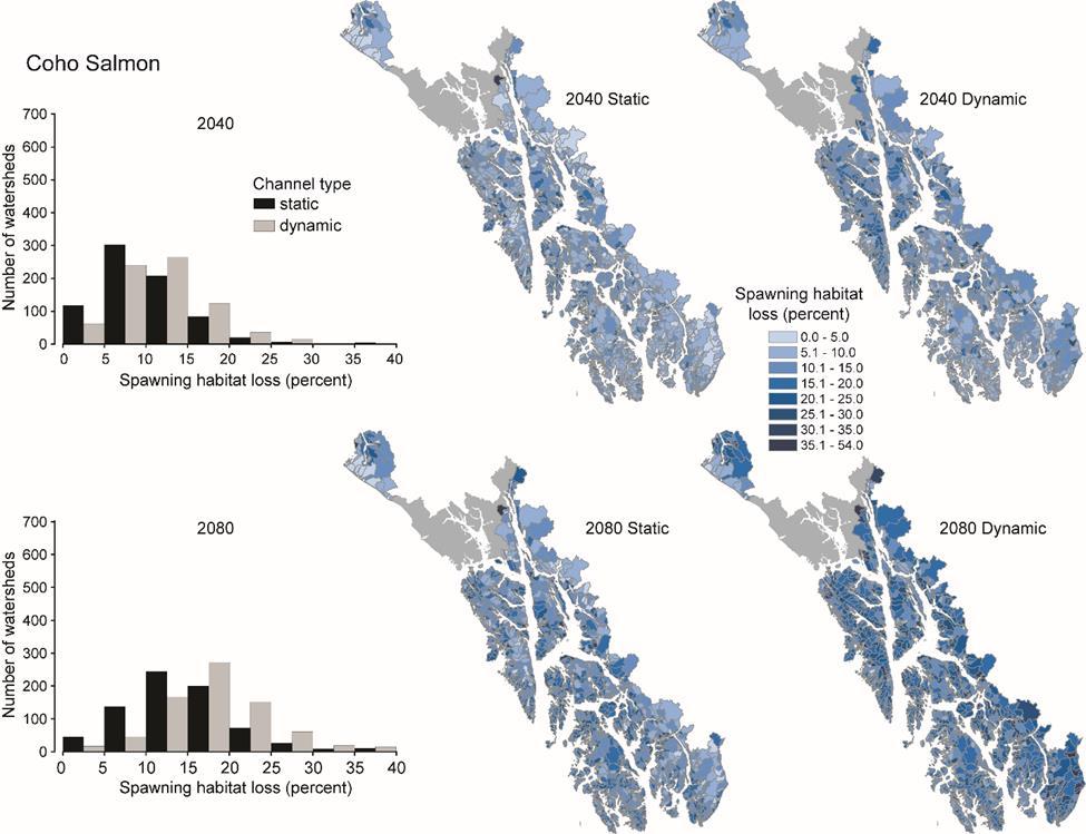
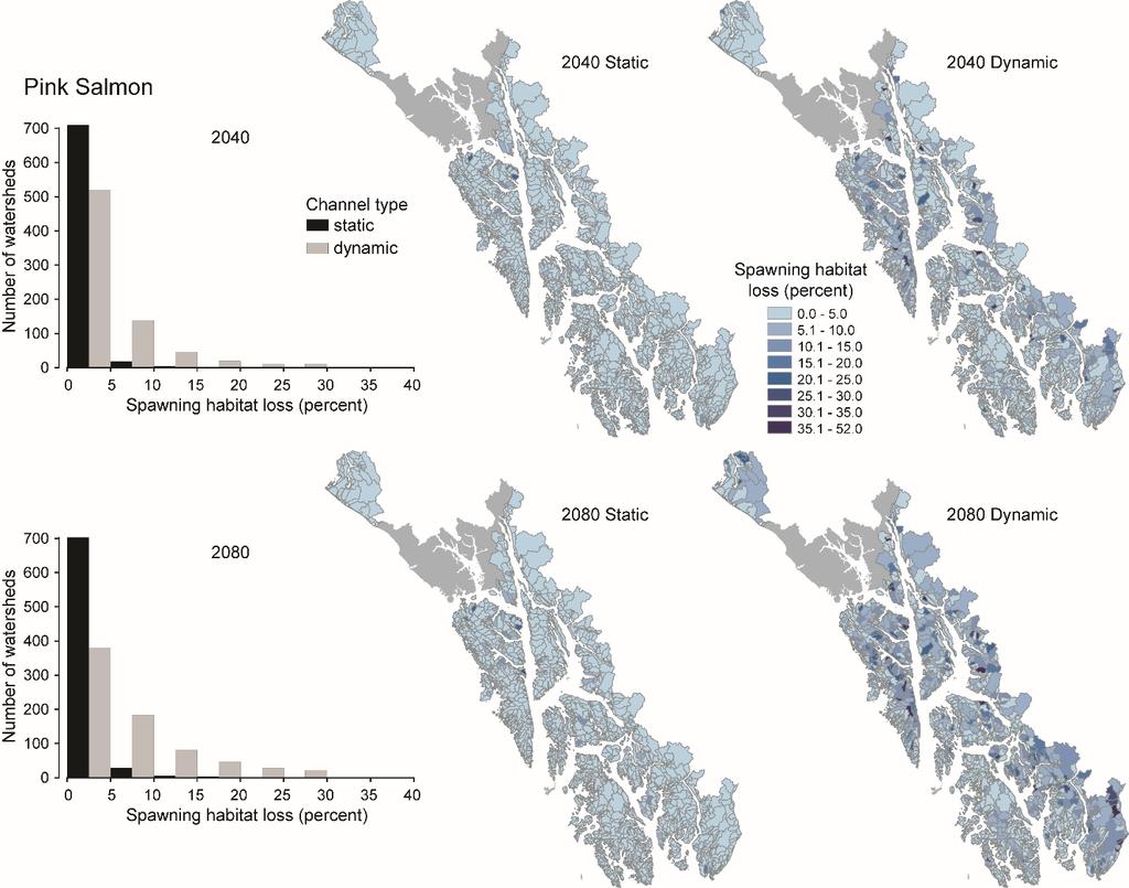
33 A. static B. dynamic

34

35 Conclusions: Mean annual flood magnitudes may increase ~18% and 28% by the 2040s and 2080s (high spatial variability). Exposure to flow change is not necessarily a good measure of vulnerability. Expect high response diversity largely driven by topographic and geomorphic complexity and species habitat preferences. Geomorphic context is extremely important for understanding stream habitat vulnerability to climate change.

36 Next steps? Framework can accommodate improved data quality. Incorporation into life cycle models. Integration with other disturbance models (stochastic input of sediment and wood, etc.).

37