Nitrogen cycles: past, present, and future

Transcription

1 Biogeochemistry 70: , Ó 2004 Kluwer Academic Publishers. Printed in the Netherlands. -1 Nitrogen cycles: past, present, and future J.N. GALLOWAY 1, *, F.J. DENTENER 2, D.G. CAPONE 3, E.W. BOYER 4, R.W. HOWARTH 5, S.P. SEITZINGER 6, G.P. ASNER 7, C.C. CLEVELAND 8, P.A. GREEN 9, E.A. HOLLAND 10, D.M. Karl 11, A.F. MICHAELS 3, J.H. PORTER 1, A.R. TOWNSEND 8 and C.J. VO RO SMARTY 9 1 Environmental Sciences Department, University of Virginia, Charlottesville, 22903, USA; 2 Joint Research Centre, Institute for Environment and Sustainability Climate Change Unit, Ispra, Italy; 3 Wrigley Institute for Environmental Studies, University of Southern California, Los Angeles, California, USA; 4 College of Environmental Science and Forestry, State University of New York, Syracuse, New York, USA; 5 Department of Ecology and Evolutionary Biology, Cornell University, Ithaca, New York, USA; 6 Institute of Marine and Coastal Sciences, Rutgers, The State University of New Jersey, New Brunswick, New Jersey, USA; 7 Department of Global Ecology, Carnegie Institution, Stanford University, Stanford, California, USA; 8 Institute of Arctic and Alpine Research, University of Colorado, Boulder, Colorado, USA; 9 Complex Systems Research Center, Institute for the Study of Earth, Oceans, and Space, University of New Hampshire, Durham, New Hampshire, USA; 10 Atmospheric Chemistry Division, National Center for Atmospheric Research, Boulder, Colorado, USA; 11 School of Ocean and Earth Science and Technology, University of Hawaii, Honolulu, Hawaii, USA; *Author for correspondence ( jng@virginia.edu; phone: ; fax: ) Received 14 March 2003; accepted in revised form 1 March 2004 Key words: Denitrification, Fertilizer, Fossil fuel combustion, Haber-Bosch, Nitrogen, Nitrogen fixation Abstract. This paper contrasts the natural and anthropogenic controls on the conversion of unreactive N 2 to more reactive forms of nitrogen (Nr). A variety of data sets are used to construct global N budgets for 1860 and the early 1990s and to make projections for the global N budget in Regional N budgets for Asia, North America, and other major regions for the early 1990s, as well as the marine N budget, are presented to highlight the dominant fluxes of nitrogen in each region. Important findings are that human activities increasingly dominate the N budget at the global and at most regional scales, the terrestrial and open ocean N budgets are essentially disconnected, and the fixed forms of N are accumulating in most environmental reservoirs. The largest uncertainties in our understanding of the N budget at most scales are the rates of natural biological nitrogen fixation, the amount of Nr storage in most environmental reservoirs, and the production rates of N 2 by denitrification. Introduction Water, water everywhere, and all the boards did shrink; Water, water everywhere, nor any drop to drink. This couplet from the Rime of the Ancient Mariner (Samuel Taylor Coleridge, ) is an observation that, although sailors were surrounded by

2 154 water, they were dying of thirst because of its form. Just as water is a critical substance for life, so is nitrogen. And just as most of the water on the planet is not useable by most organisms, most of the nitrogen is also unavailable. Approximately 78% of the atmosphere is diatomic nitrogen (N 2 ), which is unavailable to most organisms because of the strength of the triple bond that holds the two nitrogen atoms together. Over evolutionary history, only a limited number of species of Bacteria and Archaea have evolved the ability to convert N 2 to reactive nitrogen (Nr) 1. However, even with adaptations to use nitrogen efficiently, many ecosystems of the world are limited by nitrogen. To place the current alteration of N cycle into historical context, we begin this review with a brief history of the development of human understanding of the nitrogen cycle. We use as a primary reference Smil (2001) which thoroughly documents the history of N as part of a discussion of the Haber-Bosch process. Jean Antoine Claude Chaptal ( ) formally named the 7th element of the periodic table in By the beginning of the second half of the 19th century, it was known that N was a common element in plant and animal tissues, that it was indispensable for plant growth, that there was constant cycling between organic and inorganic compounds, and that it was an effective fertilizer. However, the source of nitrogen was uncertain. Lightning and atmospheric deposition were thought to be the most important sources. Although the existence of biological nitrogen fixation (BNF) was unknown, in 1838 Boussingault demonstrated that legumes could restore Nr to the soil and that somehow they must create Nr directly. It was 50 more years before the puzzle was solved. In 1888 Herman Hellriegel ( ) and Hermann Wilfarth ( ) published their work on microbial communities: The Leguminosae do not themselves possess the ability to assimilate free nitrogen in the air, but the active participation of living micro-organisms in the soil is absolutely necessary (Smil 2001). They went on to say that it was necessary that there was a symbiotic relationship between legumes and micro-organisms. Also around this time, the processes of nitrification and denitrification were identified so, by the end of the 19th century, the essential components of the nitrogen cycle were in place. Over the past 100 years, our knowledge of Nr creation and its movement through ecosystems and environmental reservoirs has increased dramatically. We know that Nr creation occurs in a number of ecosystems (via BNF) as well as by lightning. We also know that the productivity of many ecosystems is controlled by N availability (Vitousek et al. 2002). Although this limitation is part of the natural process, it was not tenable for a growing human population 1 The term reactive nitrogen (Nr) as used in this paper includes all biologically active, photochemically reactive, and radiatively active N compounds in the atmosphere and biosphere of the Earth. Thus Nr includes inorganic reduced forms of N (e.g., NH 3,NH 4 + ), inorganic oxidized forms (e.g., NO x, HNO 3,N 2 O, NO 3 ), and organic compounds (e.g., urea, amines, proteins, nucleic acids). Note that this definition is much broader than the term reactive N as defined by the atmospheric chemistry community they define reactive N as NO y, which is any N O combination except N 2 O (e.g., NO x,n 2 O 5, HNO 2, HNO 3, nitrates, organic nitrates, halogen nitrates, etc).

3 155 that needed increasing amounts of Nr to grow food. This demand has resulted in a very significant alteration of the N cycle in air, land, and water and at local, regional, and global scales. Two anthropogenic activities have greatly increased Nr availability. The first is food production. Early hunter-gatherer peoples were able to meet their nitrogen requirements by consuming protein from wild plants and animals. However, the establishment of settled communities 10,000 years ago required the ability to grow your own. Archeological evidence points to legume cultivation over 6500 years ago (Smith 1995). Rice cultivation began in Asia perhaps as early as 7000 years ago (Wittwer et al. 1987), and soybeans have been cultivated in China for at least 3100 years (Wang 1987). These crops resulted in anthropogenic-induced creation of Nr since legumes can self-fertilize via symbioses with N 2 -fixing organisms and rice cultivation creates anaerobic environments that encouraged high rates of BNF by cyanobacteria. The annual per-area rates of transfer of atmospheric N 2 to Nr by cultivation can be large compared to natural rates of transfer. As thoroughly reviewed by Smil (1999), Rhizobium associated with seed legumes (e.g., peas and beans) can fix N at rates ranging from to mg N m 2. Most fixation rates are on the order of to mg N m 2. Rhizobium associated with leguminous forages (e.g., alfalfa, clover) have higher average rates, to mg N m 2. Non-Rhizobium N-fixing organisms associated with some crops (e.g., cereals) and trees have ranges from to mg N m 2, while cyanobacteria associated with rice paddies and endophytic diazotrophs associated with sugar cane can fix to mg N m 2 and , respectively (Smil 1999). The second anthropogenic activity that increased Nr was energy production. Although food production creates additional Nr on purpose, energy production creates it by accident (H. Levy, personal communication, 1995). During combustion of fossil fuels nitrogen is emitted to the atmosphere as a waste product (NO) from either the oxidation of atmospheric N 2 or organic N in the fuel (primarily coal) (Socolow 1999; Galloway et al. 2002). The former creates new Nr; the latter mobilizes sequestered Nr. The magnitude of Nr mobilization due to energy production is not as extensive as that from food production. Although there are records of coal use dating from 500 BC in China, up until the late 19th century most energy was produced from biofuels (e.g., wood). It was not until the beginning of the 20th century that fossil fuels overtook biomass fuels in supplying primary energy (Smil 1994). By the beginning of the 20th century the importance of nitrogen in food production had been established and the major components of the N cycle had been identified. In addition, both legume/rice cultivation and fossil fuel combustion were creating Nr: the former as a means to provide N to produce food and the latter as a consequence of energy production. Many realized that there was not enough nitrogen available from naturally occurring sources to provide food for a growing global population (Smil 2001). The only sources for new N at that time (in addition to cultivation) were guano deposits on arid islands and

4 156 evaporite nitrate deposits in South America (e.g., Chile), which supplied about 0.2 Tg N yr 1 (Smil 2000). This was not enough. The pressure to obtain additional Nr for food production (and the need for nitrate to produce munitions) led to the 1913 development of the Haber-Bosch process in Germany to produce NH 3 from N 2 and H 2 (Smil 2001). We are now at the beginning of the 21st century. Food and energy production have grown with population and, in some regions, with significant increases in the per-capita resource use. Currently, food and energy production has increased the anthropogenic Nr creation rate by over a factor of 10 compared to the late-19th century. The magnitude of this production raises critical questions as to the consequences and fate of new Nr in the environment. Answers to these questions are problematic. With seven oxidation states, numerous mechanisms for interspecies conversion, and a variety of environmental transport/storage processes, nitrogen has arguably the most complex cycle of all the major elements. This complexity makes tracking anthropogenic nitrogen through environmental reservoirs a challenge. However, such work is necessary because of nitrogen s role in all living systems and in several environmental issues (e.g., greenhouse effect, smog, stratospheric ozone depletion, acid deposition, coastal eutrophication and productivity of freshwaters, marine waters, and terrestrial ecosystems). The analysis of the magnitude and consequences of human intervention in the N cycle is not new. More than 30 years ago, Delwiche (1970) stated that humans were mobilizing about the same amount of N as natural processes and that the fate of the new Nr was uncertain. Since Delwiche s seminal work, anthropogenic Nr creation has doubled while natural terrestrial BNF has decreased due to land use change. Many uncertainties remain and have become all the more important to resolve. In the last several years, a number of recent papers have addressed the N cycle on a global scale (e.g., Ayres et al. 1994; Mackenzie 1994; Galloway et al. 1995; Vitousek et al. 1997; Galloway 1998; Seitzinger and Kroeze 1998; Galloway and Cowling 2002); a regional scale (Asia Galloway 2000; Zheng et al. 2002; Bashkin et al. 2002; North Atlantic Ocean and watershed Galloway et al. 1996; Howarth et al. 1996; oceans Karl 1999; Capone 2001; Karl et al. 2002; Europe van Egmond et al. 2002; United States Howarth et al. 2002); and on major components of the N cycle (food production Smil 1999, 2002; Oenema and Pietrzak 2002; Cassman et al. 2002; Roy et al. 2002; fertilizer production Fixen and West 2002; fossil fuel combustion Bradley and Jones 2002; Moomaw 2002; industrial uses of Nr Febre Domene and Ayres 2001; the atmosphere Holland et al. 1999; BNF Cleveland et al. 1999; Karl 1999, 2002; Vitousek et al. 2002) and its relationship to public policy (Socolow 1999; Mosier et al. 2001; Melillo and Cowling 2002). Using these previous papers as a foundation, the results of the multi-year SCOPE project (Boyer and Howarth 2002), and the findings of the Second International Nitrogen Conference (Galloway et al. 2002), this paper addresses the following questions:

5 157 How has the global nitrogen budget changed from the late 19th century to the late 20th century? What is the global N budget projected to be in the mid-21st century? How have atmosphere-biosphere N exchanges been altered by human activity? What are the connections between the terrestrial and marine N cycles? How much of the Nr created by human activity is denitrified back to N 2? These are important questions to address. Nr influences biogeochemical processes in the atmosphere, in terrestrial ecosystems, and in freshwater and marine aquatic ecosystems. Increases in the concentration of Nr species can enhance ecosystem productivity through fertilization or decrease it through nutrient imbalances and decrease ecosystem biodiversity through acidification and eutrophication (Vitousek et al. 1997; Aber et al. 1998; NRC 2000; Matson et al. 2002; Rabalais 2002; Tartowski and Howarth 2000). Higher Nr concentrations in the atmosphere can increase the incidence of air-pollution-related illness due to O 3 and particulate matter inhalation (Follett and Follett 2001; Wolfe and Patz 2002; Townsend et al. 2003). A unique aspect of the impact of Nr on the environment and on people is that the effects can occur in series. Referred to as the nitrogen cascade (Galloway et al. 2003), one atom of nitrogen can, in sequence, increase atmospheric O 3 (human health impact), increase fine particulate matter (visibility impact), alter forest productivity, acidify surface waters (biodiversity loss), increase coastal ecosystem productivity, promote coastal eutrophication, and increase greenhouse potential of the atmosphere (via N 2 O production). The magnitude of the consequences, coupled with the magnitude of current rates of Nr creation, makes the issue of Nr accumulation an important one to address. This paper begins with the global N budget and the primary natural process that creates Nr BNF. After assessing natural terrestrial rates of Nr creation, this paper addresses anthropogenic Nr creation rates in 1860 and the early 1990s (defined as 1990 to 1995, depending on the data set). The next two sections track Nr through global terrestrial systems for both time periods. The next section addresses the N budget on regional scales as geopolitical units. Such an analysis illustrates the spatial heterogeneity in both Nr creation and distribution. This paper then presents an assessment of the marine component of the N budget and its linkages with the terrestrial component. The final section discusses projections for the N budget in The budgets presented in this paper are constructed from data previously published (or data previously published but adjusted for the time periods covered in this paper) and data that are presented for the first time. In general, previously published data and time-adjusted data are: Nr creation by Haber- Bosch process; terrestrial BNF; cultivation-induced BNF; atmospheric emission for NO x,nh 3 and N 2 O; and NO y and NH x deposition. The marine N budget terms are based upon an assessment presented in this paper using data from a number of sources. The riverine fluxes represent a new analysis and are based primarily on other data bases used in this paper. Estimates for N 2 production via

6 158 denitrification from soils, rivers, and estuaries are based upon previously published data as well as assessments presented in this paper. Additional information about data sources is provided in the appropriate sections. The data and model results used in this paper have differing levels of uncertainty, which we have presented to the degree possible. Because of these uncertainties, we generally present fluxes to three significant figures or 0.1 Tg Nyr 1. This practice at times produces sums that are slightly different due to rounding errors from what would be obtained by numerical addition. The uncertainty associated with most fluxes is discussed within the paper. The uncertainties associated with the atmospheric NO y and NH x budgets (emissions, transport, transformation, deposition) are discussed in Appendix I. Terrestrial Nr creation Natural Lightning High temperatures occurring in lightning strikes produce NO in the atmosphere from molecular oxygen and nitrogen. Subsequently this NO is oxidized to NO 2 and then to HNO 3 and quickly (i.e., days) removed by wet and dry deposition thus introducing Nr into ecosystems primarily over tropical continents. Most current estimates of Nr creation by lightning range between 3 and 10 Tg N yr 1 (Prather et al. 2001). In this analysis we use a global estimate of 5.4 Tg N yr 1 (Lelieveld and Dentener 2000) (Table 1). Although this number is small relative to terrestrial BNF, it can be important for regions that do not have other significant Nr sources. It is also important because it creates NO x high in the free troposphere compared to NO x emitted at the earth s surface. As a result it has a longer atmospheric residence time and is more likely to contribute to tropospheric O 3 formation, which significantly impacts the oxidizing capacity of the atmosphere. BNF Problems and uncertainties. Quantifying the magnitude of natural terrestrial Nr creation by BNF is tenuous owing most notably to uncertainty and variability in the estimates of rates of BNF at the plot scale. Specifically, methodological differences, uncertainties in spatial coverage of important N-fixing species, and locational biases in the study of BNF all suggest critical gaps in our understanding of natural BNF at large scales (Cleveland et al. 1999). In addition, for many large areas where BNF is likely to be important, particularly in the tropical regions of Asia, Africa, and South America, there are virtually no data on natural terrestrial rates of BNF. In a recent compilation of rates of natural BNF by Cleveland et al. (1999), symbiotic BNF rates for several biome types are based on one-to-few published rates of symbiotic BNF at the plot scale within each particular biome. For example, based on the few estimates of symbiotic

7 159 Table 1. Global Nr creation and distribution, Tg N yr Early-1990s 2050 Notes Nr creation 1 Natural Lightning BNF-terestrial BNF-marine Subtotal Anthropogenic Haber-Bosch BNF-cultivation Fossil fuel combustion Subtotal Total Atmospheric emission 2 NO x Fossil fuel combustion Lightning Other emissions NH 3 Terrestrial Marine N 2 O Terrestrial ±? Marine Total (NO x and NH 3 ) Atmospheric deposition 3 NO y Terrestrial Marine Subtotal NH x Terrestrial Marine Subtotal Total Riverine fluxes 4 Nr input into rivers Nr export to inland systems Nr export to coastal areas Denitrification 5 Continental Terrestrial Riverine Subtotal Estuary and shelf Riverine nitrate Open ocean nitrate Subtotal

8 160 Table 1. Continued 1860 Early-1990s 2050 Notes Open ocean Total Notes 1. Nr creation BNF-terrestial based on Cleveland et al. (1999) as discussed in the text. BNF-marine Table 9 (average of the minimum and maximum values). Lightning Lelieveld and Dentener (2000). Haber-Bosch early-1990s (Kramer 1999); 2050 (see text). BNF cultivation based on Smil (1999; pers. comm.) Combustion Klein Goldewijk and Battjes (1997); van Aardenne et al. (2001). 2. Atmospheric emission NO x (other emissions) Klein Goldewijk and Battjes (1997); van Aardenne et al. (2001). NH 3 see text. N 2 O see text. 3. Atmospheric deposition NO x and NH x see text. 4. Riverine fluxes Nr inputs into rivers assumed to be twice riverine discharge. Range is 30 70% (Seitzinger et al. 2000). River fluxes see text and Appendix II. 5. Denitrification Terrestial 1860, no storage; 1990s, natural denitrification reduced, 0.25 of anthropogenic Nr is denitrified, and excess river N is discharged. Riverine assumed to be equal to difference between river input and river discharge. Estuary and Shelf Shelf estimate (Table 9) minus 1860 riverine discharge. BNF available for tropical rain forests, estimated BNF in these systems represents 24% of total natural terrestrial BNF globally on an annual basis (Cleveland et al. 1999). While the relative richness of potential N 2 -fixing legumes in tropical forests suggests that symbiotic BNF in these systems is relatively high (Crews 1999), the paucity of actual BNF rate estimates in these systems suggests caution when attempting to extrapolate plot scale estimates of BNF and highlights the difficulties of attempting to estimate natural BNF at the global scale. Previous estimates. Difficulties notwithstanding, prior estimates of BNF in terrestrial ecosystems range from 40 to 200 Tg N yr 1 (e.g. Schlesinger 1991; So derland and Rosswall 1982; Stedman and Shetter 1983; Paul and Clark 1997). Most studies merely present BNF estimates as global values that, at best, are broken into a few very broad components (e.g., forest, grassland, and other; e.g., Paul and Clark 1997). Such coarse divisions average enormous land areas that contain significant variation in both BNF data sets and biome types thus diminishing their usefulness. Many studies do not list the data sources from which their estimates were derived (e.g., Schlesinger 1991; So derland and Rosswall 1982; Stedman and Shetter 1983; Paul and Clark 1997). In contrast, Cleveland et al. (1999) provided a range of estimates of BNF in natural ecosystems from 100 to 290 Tg N yr 1 (with a best estimate of 195 Tg N yr 1 ). These

9 161 estimates were based on published, data-based rates of BNF in natural ecosystems and differ only in the percent cover estimates of symbiotic N fixers used to scale plot-level estimates to the biome scale. Current estimates. Although the data-based estimates of Cleveland et al. (1999) provide more documented, constrained range of terrestrial BNF, there are several compelling reasons to believe that an estimate in the lower portion of the range is more realistic than higher estimates. First, rate estimates of BNF presented in the literature are inherently biased, as investigations of BNF are frequently carried out in areas where BNF is most likely to be important (i.e., where there are large assemblages of N-fixing species that do not reflect average community composition for the entire biome). For example, many rates of BNF in temperate forests were derived from studies that include N inputs from alder and black locust (Cleveland et al. 1999). Although rates of BNF may be very high within stands dominated by these species (Boring and Swank 1984; Binkley et al. 1994), these species are certainly not dominant in temperate forests as a whole (Johnson and Mayeux 1990). Similarly, although species with high rates of BNF are often common in early successional forests (Vitousek 1994), they are often rare in mature or late successional forests, especially in the temperate zone (Gorham et al. 1979; Boring and Swank 1984; Blundon and Dale 1990). Literature-derived estimates based on reported coverage of N-fixing species are thus inflated due to these inherent biases. We suggest that annual global BNF contributed between 100 and 290 Tg Nyr 1 to natural terrestrial ecosystems prior to large-scale human disturbance. However, we contend that, due to the inherent biases noted in plot-scale studies of N fixation rates, the true rate of BNF lies at the lower end of this range. Thus, we used actual evapotranspiration (ET) values generated in Terraflux (Asner et al. 2001; Bonan 1996) and the strong, positive relationship between ET and BNF (Cleveland et al. 1999) to generate a new, single estimate of BNF prior to large-scale human disturbance. Our new analysis is based on the relationship between ET and BNF but uses rates of BNF calculated using the low percent cover values of symbiotic N fixers over the landscape (i.e., 5%; Cleveland et al. 1999). This analysis suggests that within the range of 100 to 290 Tg N yr 1, natural BNF in terrestrial ecosystems contributes 128 Tg Nyr 1. This value is supported by an analysis comparing BNF to N requirement (by biome type). Using the Cleveland et al. (1999) relationship between ET and BNF, a global N fixation value of 128 Tg N yr 1 would suggest an average of 15% of the N requirement across all biome types is met via BNF; higher estimates of BNF would imply that at least 30% of the N requirement across all biomes is met via natural BNF (Asner et al. 2001). However, BNF in even the most active leguminous crop species frequently accounts for <30% of total plant N (Peoples et al. 1995). Our estimate (128 Tg N yr 1 ) represents potential BNF prior to large-scale human disturbance and does not account for decreases in BNF due to land use change or decreases in BNF due to other physical, chemical, or biological

10 162 factors. To estimate natural terrestrial BNF for 1860 and the early-1990s, we scale BNF to the extent of altered land at those two times. Of the 11,500 million ha of natural vegetated land (Mackenzie 1998), Houghton and Hackler (2002) estimate that in 1860 and 1995, 760 million ha and 2,400 million ha, respectively, had been altered by human action (e.g., cultivation, conversion of forests to pastures). Therefore, in this analysis of BNF in the natural terrestrial landscape, we use 128 Tg N yr 1 for the natural world, 120 Tg N yr 1 for 1860, and 107 Tg N yr 1 for the present world. Summary. The conversion of N 2 to Nr requires energy to break the N:N triple bond. In the natural world, physical (lightning) and biological (BNF) processes provide this energy. Nr creation by lightning is highest in tropical terrestrial regions where convective activity is the largest. BNF rates in terrestrial systems are also generally highest in tropical regions; in contrast to many temperate forests, old-growth primary tropical rain forests often contain many potentially N-fixing canopy legumes (Cleveland et al. 1999; Vitousek et al. 2002). Thus, relative to temperate regions, tropical regions are important source areas of Nr due in part to ecosystem structure and energy availability. As will be seen in the next section, human Nr creation in many temperate regions is primarily controlled by a different factor the use of fossil energy to produce energy and fertilizer. Thus the latitude dependency changes from one driven by solar intensity and ecosystem type to one driven by population density and industrial productivity. Anthropogenic 1860 Van Aardenne et al. (2001) estimated 0.6 Tg N yr 1 of Nr was created in the form of NO x during fossil fuel combustion in 1890, primarily from coal combustion. Scaling this estimate by population and other factors, we estimate that in 1860 the equivalent value was 0.3 Tg N yr 1. Since the Haber-Bosch process was not yet invented, the only new N created by food production was by cultivation of legumes. Galloway and Cowling (2002) estimate, using assessments by V. Smil (pers. comm.), that 15 Tg N yr 1 was produced in 1900 by cultivation-induced BNF. Given the uncertainty about this estimate, we believe it to be reasonable to use this value to represent conditions in Thus before the 20th century, humans created new Nr almost entirely to support food production. The total anthropogenic Nr produced (15 Tg Nyr 1 ) was small relative to BNF occurring in unmanaged terrestrial ecosystems (120 Tg N yr 1 ) (Table 1). Early 1990s Between 1860 and 1995 the world s population increased 4.5-fold, from 1.3 to 5.8 billion. Cultivation-induced Nr creation increased by only 2-fold from

11 Tg N yr 1 in 1860 to 33 Tg N yr 1 in the mid-1990s (Smil 1999). Symbiotic BNF by Rhizobium associated with seed legumes resulted in 10 Tg N yr 1 (8 12 Tg N yr 1 ) of new nitrogen. Biofixation by leguminous cover crops (forages and green manures such as clover, alfalfa, vetches) accounted for an additional 12 Tg N yr 1 (10 14 Tg N yr 1 ) of new nitrogen. As Smil notes, biofixation by non-rhizobium N-fixing species was of less importance, fixing on the order of 4 Tg N yr 1 (2 6 Tg N yr 1 ). Cyanobacteria fixed on the order of 4 6 Tg N yr 1 in wet-rice fields, while endophytic N-fixing organisms in sugar cane fixed an additional 1 3 Tg N yr 1. The global total from cultivation is thus 33 Tg N yr 1 within a range of Tg N yr 1 (Smil 1999). When we applied Smil s crop-specific mean fixation rates to the crop area data on a regional basis from FAO (2002), we estimate that for 1995 that total global C-BNF was 31.5 Tg N yr 1, very similar to Smil s value of 33 Tg N yr 1 (Table 1). Relative to cultivation-induced BNF, about three times as much Nr was created with the Haber-Bosch process. In 1995, 100 Tg N of NH 3 was created for food production and other industrial activities (Kramer 1999). Of this amount, about 86% (86 Tg N yr 1 ) was used to make fertilizers. The remaining 14 Tg N yr 1 was dispersed to the environment during processing or used in the manufacture of synthetic fibers, refrigerants, explosives, plastics, rocket fuels, nitroparaffins, etc. (Smil 1999; Febre Domene and Ayres 2001). As with the production of fertilizer, this also represents creation of new Nr that is introduced into environmental systems. The increase in energy production by fossil fuels resulted in increased NO x emissions from 0.3 Tg N yr 1 in 1860 to 24.5 Tg N yr 1 in the early 1990s by the early 1990s over 90% of energy production resulted in the creation of new reactive nitrogen, contrasting to 1860 where very little of energy production caused creation of Nr. Summary In the early 1990s, Nr creation by anthropogenic activities was 156 Tg Nyr 1, a factor of 10 increase over 1860, contrasted to only a factor of 4.5 increase in global population (Table 1). Food production accounted for 77%, energy production accounted for 16%, and production for industrial uses accounted for 9%. Global terrestrial N budget Introduction This section examines the extent of Nr distribution via atmospheric and hydrologic pathways. It provides a context to evaluate the extent to which human intervention in the N cycle in the early 1990s has substantially changed N distribution on a global and regional basis. The global fluxes presented in

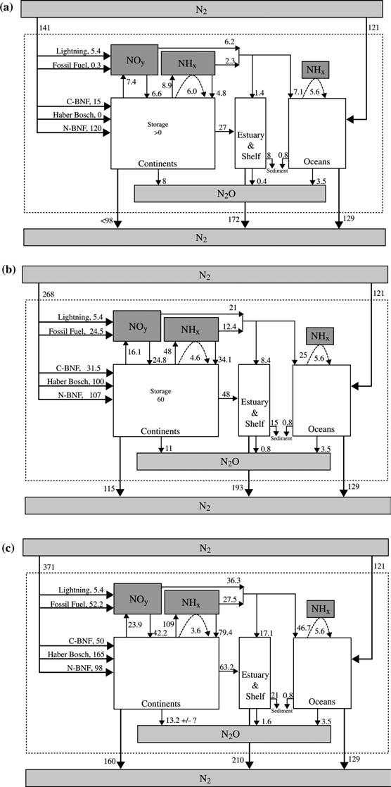
12 164 this section represent an update and an expansion over those presented in Galloway and Cowling (2002) Fixation As discussed above, natural rates of Nr creation in 1860 were 120 Tg N yr 1 by terrestrial BNF and 5.4 Tg N yr 1 by lightning. Anthropogenic Nr creation rates were 0.3 and 15 Tg N yr 1 by fossil fuel combustion and cultivationinduced terrestrial BNF, respectively. Total terrestrial Nr creation was 141 Tg N yr 1 (Figure 1a, Table 1). Emission and deposition Atmospheric emissions for 1860 and 1993 (except for marine NH 3 emissions) were derived from a 1 1 data-base (van Aardenne et al. 2001) that covered 1890 to The adjustment to 1860 used estimated activity data (e.g., population) together with emission factors for For 1993 we extrapolated 1990 anthropogenic emissions using the reported increase of CO 2 emissions for the period (Brenkert 1997). Emission factors were assumed to be unchanged. Marine NH 3 emissions are based on the monthly oceanic NH 4 + and ph values derived from the HAMOCC3 biological ocean model (for further information see Bouwman et al. (1997) and Quinn et al. (1996)) and model-calculated exchange velocities. The atmospheric deposition data on a 5 by 3.75 grid were generated from a global transport-chemistry model (Lelieveld and Dentener 2000). Each grid was subdivided into a 50 km 50 km sub-grid to create a spatially defined deposition map (Figure 2). The gridded data were assigned to continental and marine regions needed for this study using boundaries delineated on a world data coverage from ESRI (1993). (See Appendix I for a discussion of uncertainties in these estimates.) NO x and NH 3 emissions can result from natural processes, food production, and energy production. Although the anthropogenic creation rate of Nr was only 16% of that created naturally in terrestrial environments, in 1860 humans had an observable effect on atmospheric Nr emissions. For NO x, Figure 1. Components of the global nitrogen cycle for (a) 1860, (b) early 1990s, and (c) 2050, Tg Nyr 1. All shaded boxes represent reservoirs of nitrogen species in the atmosphere. Creation of Nr is depicted with bold arrows from the N 2 reservoir to the Nr reservoir (depicted by the dotted box). N-BNF is biological nitrogen fixation within natural ecosystems, C-BNF is biological nitrogen fixation within agroecosystems. Denitrification creation of N 2 from Nr within the dotted box is also shown with bold arrows. All arrows that do not leave the dotted box represent inter-reservoir exchanges of Nr. The dashed arrows within the dotted box associated with NH x represent natural emissions of NH 3 that are re-deposited on fast time-scales to the oceans and continents. c

13 165

14 166 Figure 2. Spatial patterns of total inorganic nitrogen deposition in (a) 1860, (b) early 1990s, and (c) 2050, mg N m 2 yr 1.

15 167 natural emissions occur from soil processes, lightning, wildfires (biomass burning), and stratospheric injection. These amounted to a total of 10.5 Tg yr 1 (Table 2). Energy production resulted in total NO x emissions of 0.6 Tg Nyr 1, (0.3 Tg N yr 1 from fossil fuel combustion and 0.4 Tg N yr 1 from biofuel combustion). Food-production-related combustion of agricultural waste yielded 0.9 Tg N NO x yr 1. Slash-and-burn of forests yielded 0.2 Tg Nyr 1, and the annual burning of savanna grass and shrubs emitted 0.9 Tg N yr 1. In 1860, total NO x emissions were 13.1 Tg N yr 1 of which 10.5 Tg N yr 1 were from natural sources. Total NO y deposition is 12.8 Tg Nyr 1 (Table 2), with 6.6 Tg N yr 1 to continents and 6.2 Tg N yr 1 to oceans (Table 1). The equivalent analysis for NH 3 shows that energy production resulted in 0.7 Tg N yr 1 from the combustion of biofuels (Table 2). Food production resulted in NH 3 emissions to the atmosphere of 6.6 Tg N yr 1, 10-fold greater than energy production. The component parts were combustion of agricultural waste (0.6 Tg N yr 1 ), forests (0.2 Tg N yr 1 ), and savannas (0.2 Tg N yr 1 ). Low-temperature NH 3 emissions were 5.3 Tg N yr 1 from domestic animal waste, 0.1 Tg N yr 1 from human sewage, and 0.2 Tg N yr 1 from crops (Table 2). Natural emissions of NH 3 from oceans and natural vegetation were calculated using a compensation point approach. This results in a net exchange of NH 3 between the atmosphere and the underlying surface (Dentener and Crutzen 1994; Conrad and Dentener 1999). These emissions were part of a rapid local cycling, meaning that most of the emissions are deposited within the same region (Table 2) as illustrated with the dotted arrows in Figure 1a. Deposition of NH x to the continents from non-local sources was 4.8 Tg N yr 1 and to the ocean, 2.3 Tg N yr 1. Including the rapid deposition of the natural NH 3 emissions, these numbers would have been 10.8 and 7.9 Tg N yr 1 to continents and oceans, respectively, in 1860 (Table 1). Given the contributions to atmospheric N emissions from energy and food production in contrast to natural emissions, it is not surprising that a map of N deposition for 1860 to the earth surface shows the imprint of human activity (Figure 2a). N deposition was more pronounced near populated areas with rates up to a few hundred mg N m 2 yr 1 while in more remote regions it is on the order of mg N m 2 yr 1 for terrestrial regions and 5 25 mg N m 2 yr 1 for marine regions. The largest deposition rates were in Asia (maximum on the order of 1000 mg N m 2 yr 1 ), which is not surprising as it had 65% of the world s population. The evidence of atmospheric transport downwind from these areas is also evident (Figure 2a). Another Nr species emitted to the atmosphere, N 2 O, bears mention. In 1860 terrestrial systems contributed 6.6 Tg N yr 1 (assuming the Bouwman et al. (1995) natural soil emissions for 1990 are applicable to 1860 conditions) (Table 3). As noted in Kroeze et al. (1999), anthropogenic N 2 O emissions from animal waste, cultivation-induced BNF, crop residue, and biomass burning were approximately 1.4 Tg N yr 1. Rivers are estimated to have contributed another 0.05 Tg N yr 1 (Seitzinger et al. 2000). Estuaries and marine shelves

16 168 Table 2. Global atmospheric emissions of NH 3 and NO x,tg Nyr Note NO x NH 3 NO x NH 3 NO x NH 3 Food A1 Sav Agl Agr Def Fer Anm Lan Cro Subtotal Energy A2 E1* Nrt and ots* Aircraft* His Bf Subtotal Natural A3 Aglnat Lightning* Firenat Strat Soil and veg Ocean Subtotal Emission, total Deposition, total B1 Notes A. Emissions (van Aardenne et al. 2001). 1. Food sav represents NO x and NH 3 emissions from savannah burning, some fraction of which could be considered natural; agl is NO x emissions from agricultural soils; agr is NO x and NH 3 emissions from agricultural waste burning; def is NO x and NH 3 emissions from combustion, as part of deforestation; anm is NH 3 emissions from agricultural animal waste; ian is NH 3 emissions from humans, pets and waste water; cro is NH 3 emissions from agricultural crops. 2. Energy e1 is NO x and NH 3 emissions from fossil fuel burning; his is NO x and NH 3 emissions from industrial processes; nrt and ots is NO x emissions from non-road transport and one specific industrial sector; aircraft is NO x emissions from stratospheric aircraft; bf3 is non-road transport and one specific industrial sector from biofuel combustion. An asterisk means that the combustion process lead to the creation of new Nr. 3. Natural aglnat is NO x emissions from natural soils; lightning is NO x formation due to lightning; firenat is NO x and NH 3 emissions from natural burning at high latitudes; strat is NO x injection from stratosphere; soil and veg is NH 3 emissions from natural soils, vegetation and wild animals, calculated using a compensation point (see text); oceans is NH 3 emission from oceans calculated using a compensation point (see text). B. Deposition (Lelieveld and Dentener 2000). 1. Data are for wet and dry deposition of NO y and NH x (Table 1).

17 169 Table 3. Global atmospheric emissions of N 2 O, Tg N yr Early 1990s 2050 Notes Soils Natural Anthropogenic ±? 2 Rivers Natural Anthropogenic Esturaries Natural Anthropogenic Shelves Natural Anthropogenic Ocean (natural) Total ±? 8 Notes 1.We have assumed that the Bouwman et al. (1995) estimate of N 2 O emissions from natural soils for 1990s was applicable to 1860 and 2050 conditions , Kroeze et al. (1999); early 1990s, Bouwman et al. (1995). 3. Seitzinger and Kroeze 1998; Kroeze and Seitzinger 1998; Seitzinger et al Seitzinger and Kroeze 1998; Kroeze and Seitzinger 1998; Seitzinger et al Seitzinger et al. (2000). 6. Early-1990s, Seitzinger et al. (2000); 2050, Kroeze and Seitzinger (1998). 7. Our value of 3.5 was obtained by subtracting shelf N 2 O emissions from estimate of Nevison et al. (1995) for Further we assumed that Nevision et al. estimate for 1990 was applicable to 1860 and 2050 conditions. 8. The ±? reflects the uncertainity in anthropogenic emissions in accounted for 0.02 and 0.4 Tg N yr 1, respectively (Seitzinger et al. 2000), and the open ocean contributed 3.5 Tg N yr 1 (Nevison et al. 1995) (Table 3), Figure 1a). Thus total N 2 O emissions were 12 Tg N yr 1 in N 2 Ois globally distributed and either accumulates in the troposphere or is lost to the stratosphere (Prather et al. 2001). Although there are considerable uncertainties in the magnitude of N 2 O emissions from any one source, a closed N 2 O budget for the period is obtained when emissions from all sources are used as input to an atmospheric model indicating that increases in atmospheric N 2 O can be primarily attributed to direct and indirect emissions associated with changes in food production systems (Kroeze et al. 1999). The atmospheric portion of this analysis of the global N cycle only addresses inorganic N (NO y, NH x and N 2 O) and does not include oxidized atmospheric organic N (i.e., organic nitrates (e.g., PAN), reduced atmospheric organic N (e.g., aerosol amines and urea), and particulate atmospheric organic N (e.g., bacteria, dust)). The emission and deposition of organic N is probably a significant component of the atmospheric N cycle. Neff et al. (2002) estimate for the present time a range of Tg N yr 1 emitted and deposited on a global basis, with the range reflecting the substantial unresolved uncertainties.

18 170 Human activities certainly contribute to organic N in the atmosphere both from direct emissions and indirect (e.g., organic nitrates formation due to increased NO x emissions). However, because of the limited number of measurements, the quantification of the influence of humans has not been possible (Neff et al. 2002). Riverine export Our estimates of riverine Nr fluxes to inland-receiving waters and to the coastal ocean are based on a modification of an empirical, mass-balance model relating net anthropogenic Nr inputs per landscape area (NANI) to the total flux of Nr discharged in rivers originally established using data from land regions draining to the coastal zone of the North Atlantic Ocean (Howarth et al. 1996). The NANI model considered new inputs of Nr that are human controlled, including inputs from fossil-fuel derived atmospheric deposition, fixation in cultivated croplands, fertilizer use, and the net import (or export) in food and feed to a region. Subsequent studies have found that the form of the relationship holds when considering other world regions in the temperate zone (e.g., Boyer et al. 2002; Boyer et al. pers. comm.). Further, a model intercomparison by Alexander et al. (2002) found the NANI model to be the most robust and least biased of several models used to estimate N fluxes from a variety of large watersheds. For this paper we use a modification (as described in Appendix II and detailed in Boyer et al. (pers. comm.)) of the NANI model to quantify riverine Nr export from world regions for 1860, 1990, and The modification considers new inputs of Nr to a region from natural BNF in forests and other non-cultivated vegetated lands in addition to anthropogenic Nr inputs: the net total nitrogen inputs per unit area of landscape (or NTNI, which includes anthropogenic plus natural N inputs). Using data for a variety of coastal watersheds throughout the world, Boyer et al. (pers. comm.) found that riverine export was approximately 25% of NTNI. Aggregation of Nr input data for each region by Boyer et al. was based on the same data sources discussed in this paper (Appendix II). Using this approach, we estimate that in 1860 riverine export of total Nr to inland-receiving waters was 7.9 Tg N yr 1 and that riverine export of total Nr in waters draining to the coastal ocean was 27 Tg N yr 1. The remainder of the Nr inputs not accounted for in riverine export were stored, emitted to the atmosphere as N 2, or transported to the oceans via the atmosphere. Denitrification and storage About 30% of the 141 Tg N of terrestrial Nr created in 1860 was lost from continents: 8 Tg N of N 2 O are emitted to the atmosphere where it is stored or transported to stratosphere; 28.4 Tg N are transferred to coastal systems by rivers (27 Tg N) and atmospheric deposition (1.4 Tg N), where most is denitrified (see below); and 7.1 Tg N are deposited to the open ocean surface (Figure 1a). The remaining 98 Tg N is either stored within terrestrial systems

19 171 as a reactive species or is denitrified to N 2, the primary process that converts Nr back to its unreactive form. Note that a small portion of the denitrified Nr will not become N 2 but rather chemically (NO) or radiatively (N 2 O) important gases. The relative importance of storage versus denitrification production of N 2 is arguably the largest uncertainty that exists for nitrogen budgets at most any scale. For pristine ecosystems over long time scales, it is reasonable to propose that Nr creation should be balanced by denitrification production of N 2. This hypothesis is supported by the constancy of the atmospheric N 2 O recorded in ice bubbles back to 1000 AD, which implies that BNF and denitrification in pre-anthropogenic times were approximately equal (Ayres et al. 1994), and thus Nr was not accumulating in environmental reservoirs prior to human intervention. Although the assumption of equality between BNF and denitrification may be reasonable over the very long time scale, there is certainly significant variability year to year. Thus we choose not to make a specific estimate for 1860, except to say that the upper limit of denitrification is 98 Tg Nyr 1 or 70% of total terrestrial Nr inputs. This implies that no net Nr storage occurred in terrestrial systems. A more detailed estimate of denitrification from soils and the stream-river-estuary-shelf continuum is presented below for the present world. Summary In 1860 natural terrestrial BNF created 120 Tg N of Nr and lightning created another 5.4 Tg N. Taken together, these natural processes were 8-fold greater than the Nr created by anthropogenic activities (fossil fuel combustion, 0.3 Tg N, and cultivation-induced BNF, 15 Tg N). After accounting for the transfer to the ocean via atmosphere and rivers and the emission of N 2 O to the atmosphere, 98 Tg N yr 1 of the 141 Tg N yr 1 of new Nr created is missing and was either stored as Nr in terrestrial systems or denitrified to N 2. Early 1990s Fixation BNF by natural terrestrial ecosystems in the early 1990s was 107 Tg N yr 1 ; lightning provided a minor additional source of 5.4 Tg N yr 1. Anthropogenic activities created an additional 156 Tg N yr 1 from food and energy production (Table 1). Emission and deposition NO x emissions totaled 45.9 Tg N yr 1 in the early 1990s. Energy production accounted for 27.2 Tg N yr 1 (from fossil fuel combustion, 20.4 Tg N yr 1 ; biofuel combustion, 1.3 Tg N yr 1 ; non-road transport (e.g., ships), 3.6 Tg N yr 1 ; industrial emissions, 1.5 Tg N yr 1 ; aircraft, 0.5 Tg N yr 1 ; and miscellaneous processes, 0.7 Tg N yr 1 ) (Table 2). Food production resulted in a total of 9.0 Tg N yr 1 of NO x emissions composed of combustion of

20 172 agricultural waste (2.4 Tg N yr 1 ), forests (1.1 Tg N yr 1 ), and savanna grass (2.9 Tg N yr 1 ) and emissions from fertilized soils (2.6 Tg N yr 1 ). This final value was estimated by subtracting the 1860 NO x soil emission value from the 1993 soil emission value under the assumption that fertilizer-induced NO x emissions were trivial in Other emissions were 0.6 Tg N yr 1 coming from the stratosphere and 0.8 Tg N yr 1 from temperate wildfires (including human set fires). Total NO x emissions were 45.9 Tg N yr 1 of which 9.7 Tg Nyr 1 were from natural sources (Table 2). Total NO y deposition is 45.8 Tg Nyr 1, with 24.8 Tg N yr 1 to continents and 21.0 Tg N yr 1 to oceans (Table 1). It should be noted that there are other assessments of NO x emissions from soils larger than that used in this paper for the early 1990s (5.5 Tg Nyr 1 ). Davidson and Kingerlee (1997) estimate that global NO x emissions range from 13 to 21 Tg N yr 1. The differences in these estimates provide an indication of the uncertainty about our knowledge. Anthropogenically induced NH 3 emissions in the early 1990s totaled 47.2 Tg Nyr 1. This value is higher from that of Bouwman et al. (2002) who estimated anthropogenic NH 3 emissions in 1990 to be 43 Tg N yr 1 and lower than that of Schlesinger and Harley (1992) who estimated 52 Tg N yr 1. In our study, energy production resulted in 2.6 Tg N yr 1 from the combustion of biofuels, 0.1 Tg N yr 1 from fossil fuels, and 0.2 Tg N yr 1 from industrial sources for a total of 2.9 Tg N yr 1 (Table 2). Food production resulted in NH 3 emissions to the atmosphere of 44.3 Tg N yr 1. The component parts were combustion of agricultural waste (1.4 Tg N yr 1 ), forests (1.4 Tg N yr 1 ), and savannas (1.8 Tg N yr 1 ). Low-temperature NH 3 emissions were domestic animal waste (22.9 Tg N yr 1 ), sewage and landfills (3.1 Tg N yr 1 ), fertilizer (9.7 Tg N yr 1 ), and crops (4.0 Tg N yr 1 ). Natural emissions included high-latitude burning (0.8 Tg N yr 1 ). In addition, emissions from oceans and soils/vegetation amounted to 5.6 and 4.6 Tg N yr 1. As described before, rapid re-deposition in nearby regions effectively removes these emissions. Total NH 3 emissions were 58.3 Tg N yr 1 of which 11 Tg N yr 1 were from natural sources (Table 2). NH x deposition was 34.1 yr 1 and 12.4 Tg N yr 1 to the continents and oceans, respectively. Including the rapid deposition of the natural NH 3 emissions, these numbers would have been 38.7 Tg N yr 1 and 18 Tg N yr 1, respectively (Table 1). In the early 1990s, global atmospheric anthropogenic NH 3 and NO x emissions were 47.2 and 36.2 Tg N yr 1, respectively, which is over half of the Nr created by human action (Figure 1b). About two-thirds of the NO x emissions were a consequence of energy production (primarily fossil fuel combustion); the remainder was due to food production. About 95% of NH 3 emissions were from food production, with about half being from animal waste. For total N, about 70% of N emissions to the atmosphere are a consequence of food production. Nr deposition rates increased over a large area. In 1860, Nr deposition >750 mg N m 2 yr 1 occurred over a very small area of southern Asia (Figure 2a). In the early 1990s, large portions of North America, Europe,

21 173 and Asia had rates >750 mg N m 2 yr 1, and significant regions received >1000 mg N m 2 yr 1 (Figure 2b). Global N 2 O emissions increased from 12 Tg N yr 1 in 1860 to 15 Tg Nyr 1 in the early 1990s (Figure 1b; Table 3). Emissions from terrestrial soils and rivers were 8Tg Nyr 1 in 1860 and increased to 11 Tg N,yr 1 in 1990 primarily because of increases in N usage in food production systems. Specific sources were agricultural soils, animal-waste management systems, biomass burning, biofuel combustion, energy/transport sources, industrial processes, and rivers associated with increased N inputs from leaching (Bouwman et al. 1995). Over the same time period N 2 O emissions from estuaries and shelves also increased from 0.4 to 0.8 Tg N yr 1 mainly due to indirect agricultural effects (Seitzinger et al. 2000) Table 3, (Figure 1b) but see cautions above. Riverine export As described above and in Appendix II, riverine Nr fluxes to inland receiving waters and to coastal systems were determined using the NTNI model relating net total Nr inputs to net total Nr fluxes discharged in rivers. Accounting for about 25% of the 230 Tg N yr 1 net total Nr inputs to the terrestrial area of the continents in 1990, 11 Tg N yr 1 were transported in rivers to inlandreceiving waters and drylands not draining to coastal areas, and 48 Tg N yr 1 were transported in rivers to coastal systems. Note that the net total Nr inputs to the global watersheds (230 Tg N yr 1 ) used in the NTNI model calculation are less than the 268 Tg N yr 1 of Nr created in the early 1990s as presented in Table 1 (Figure 1b). There are three reasons for this difference. First, the NTNI model considers net anthropogenic Nr input in atmospheric deposition from fossil fuel combustion, not total atmospheric NO x emission from fossil fuel combustion. Second, the NTNI model considers net inputs of Nr in fertilizers used on the landscape. Not all the Nr created by the Haber-Bosch process is consumed as fertilizer about 14% is used for industrial purposes. Further, the amount of N fertilizer consumed on an annual basis globally is about 6% less than the amount produced (FAOSTAT 2000). Several other recent efforts have quantified global riverine Nr fluxes to the world s oceans for the 1990 timeframe. A study by Seitzinger and Kroeze (1998.) predicted global riverine Nr exports of 21 Tg Nr yr 1 even though this estimate included only the dissolved inorganic fraction of Nr export to the coastal zone. Our approach included all fractions of Nr export (total Nr: dissolved, particulate, and organic forms) and suggested a global riverine export of 48 Tg Nr yr 1. A lower global riverine loading estimate of 35 Tg Nr yr 1 was predicted by (Green et al. 2004) using data sets similar to those described herein and an empirical model relating watershed characteristics to Nr export. In contrast, a higher global riverine loading estimate of 54 Tg Nr yr 1 (total Nr) was predicted by Van Drecht et al. (2001) based on point and nonpoint sources of Nr and a model of their hydro-ecological transport and transformations. Such differences in these riverine Nr estimates highlight the

22 174 uncertainties stemming from data quality and resolution, scaling issues, and model approaches. Nr storage versus denitrification In the early 1990s, human activities created 156 Tg N yr 1 of Nr. The Nr was extensively distributed by both anthropogenic (e.g., commodity transport, see below) and natural (e.g., atmospheric and hydrologic transport) processes. Although we have a good understanding of the amount of Nr created and a reasonable understanding of its dispersion, we have a poor understanding of its ultimate fate, especially about how much is denitrified to N 2. This question is critical to answer for it limits our ability to determine the Nr accumulation rate in environmental systems. Denitrification generally requires an anoxic environment and a source of both organic matter and nitrate (Mosier et al. 2002). Thus, larger-scale hotspots for denitrification in terrestrial ecosystems tend to be characterized by high water contents (e.g., riparian zones, wetland rice, heavily irrigated regions, animal-manure holding facilities, and other wet systems such as rain-saturated soil). However, while average rates in well-drained upland systems are typically fairly low, a combination of large areas, periods of intense precipitation, and the existence of anaerobic microsites even in well-oxygenated soils can, in theory, add up to a significant potential for N 2 loss at the landscape scale. When these large, well-aerated areas are combined with smaller hotspots, significant amounts of anthropogenic Nr may be denitrified (e.g., Yavitt and Fahey 1993). Furthermore, the location and timing of denitrification in the environment may be more extensive than previously thought based on recent information on the potential for aerobic denitrification and other alternative denitrification pathways (Robertson et al. 1995; see also review by Zehr and Ward 2002). The significance of these alternative denitrification pathways in the environment is uncertain. For 1860, since we assumed that no Nr was stored in terrestrial systems, any Nr that was not lost from continents via net atmospheric losses or rivers must have been converted to N 2. For the early 1990s we present an assessment of the potential for denitrification by ecosystem type and then, at the end of the section, we rely on a limited number of landscape-scale studies to estimate N 2 production relative to Nr inputs. Atmosphere In the early 1990s, the troposphere received 46 Tg N yr 1 of NO x, 58 Tg Nyr 1 of NH 3, and 15 Tg N yr 1 of N 2 O. All of the emitted NO x and NH 3 were deposited to the earth s surface therefore there was no accumulation (or conversion back to N 2 in the atmosphere). However, 25% of the N 2 O remained in the troposphere, the remainder was destroyed in the stratosphere (Dentener and Raes, 2002). Thus of the 156 Tg N yr 1 created by human action in the early 1990s, 2.5% can be accounted for by tropospheric accumulation of N 2 O.

23 175 Forests and grasslands Temperate ecosystems historically poor in N should theoretically have a substantial capacity to store excess N, as suggested by several multiple-site studies. For example, NITREX (Dise and Wright 1992) and EXMAN (Rasmussen et al. 1990), established in Europe, manipulated the amount of Nr deposition to entire watersheds or large forest stands (Wright and Rasmussen 1998). In North America an informal collection of studies done at scales of plot to small catchments has used 15 N fertilization additions to address questions concerning the fate of Nr deposited into forests (Nadelhoffer 2001; Seely and Lajtha 1997; Nadelhoffer et al. 1992, 1995, 1999; Preston and Mead 1994). Findings from these studies support the fact that most deposited N is retained within the watershed when the inputs are fairly small, primarily in the soil. Schlesinger and Andrews (2000) reviewed several studies that assessed the fate of N added to natural ecosystems. They also found that more N accumulates in the soil than in the woody biomass. It should be noted, however, that with time some of the soil nitrogen can be later mineralized and made available to trees (Goodale et al. 2002). However, upland storage in biomass and soils can only be a transient phenomenon; at some point such sinks will begin to saturate and losses to the atmosphere and aquatic systems will rise. The timing of a transition from substantial N storage to measurable saturation of biomass and soil sinks in a system experiencing chronic elevated N loading will vary with climate, vegetation type, and pre-disturbance nutrient levels but is unlikely to exceed several decades in most ecosystems (Dise and Wright 1995; Aber et al. 1998; Fenn et al. 1998). Because of the interest in temperate forests as a potential sink for atmospheric CO 2, much of our recent information about the potential fate of excess Nr in natural ecosystems comes from northern midlatitude forests (Dise and Wright 1992; Seely and Lajtha 1997; Nadelhoffer 2001). Many studies suggest that total rates of denitrification tend to be relatively low in temperate forest soils because most are well-drained with limited anoxic regions (Gundersen 1991; Nadelhoffer 2001). However, in forest systems with high rates of N deposition not only are leaching rates increased but also gaseous losses of N are enhanced (Aber et al. 1995). For example, research at Hogwald Forest, Germany, on spruce and beech plots suggests that over a 4-year period N 2 fluxes can be a significant fraction of the N deposited (Butterbach-Bahl et al. 2002). Denitrification rates are typically larger in moist tropical forests where both moisture and nitrate levels can be substantially higher; therefore increasing N additions to tropical regions may produce more rapid and sizable denitrification losses (Matson et al. 1999). The potential for denitrification is quite large in the riparian zone of forested ecosystems where there is a supply of organic matter and a source of nitrate (Steinhart et al. 2000). Overall, as stated above, our knowledge of total potential denitrification at the scale of large forested watersheds is far too incomplete and further research in this area is sorely needed.

24 176 Finally, many of the most dramatic recent increases in atmospheric deposition to natural ecosystems have not been in temperate forests but rather in grasslands and in high-elevation and semi-arid regions (Williams et al. 1996; Asner et al. 2001). Total denitrification rates in such systems are likely to be quite low due to a combination of largely drier conditions and well-drained soils. However, our knowledge about how excess N may be partitioned in such systems, most notably semi-arid zones, is far worse than it is for temperate forests. The primary controls over the fate of N in such regions are likely to be quite different than seen in forested systems (Asner et al. 2001). There can be bursts of denitrification under certain conditions. For example, Peterjohn and Schlesinger (1991) found that there are high potential N 2 O losses from Chihuahuan desert soils (USA) after periods of rainfall. Agroecosystems Agroecosystems receive 75% of the Nr created by human action. As the amount stored within the systems each year is small relative to the amount that enters, most Nr is dispersed to other systems. Smil (1999) estimates that 170 Tg N yr 1 were added to the world s agroecosystems in the early 1990s: 120 Tg N yr 1 from the addition of new Nr (fertilizer and cultivation-induced BNF) and 50 Tg N yr 1 from the addition of existing Nr (e.g., atmospheric deposition, crop residues, animal manure). He concludes that very little of the N accumulates in the agroecosystem soil (on the order of 2 5%) and that most is either removed in the crop (50%), emitted to the atmosphere (25%), or discharged to aquatic systems (20%). This low rate of accumulation is supported by Van Breemen et al. (2002) who estimate that, for 16 large watersheds in eastern USA, only 10% of the inputs are stored within the agroecosystem. In fact, agroecosystems in some regions of the world are losing Nr. Li et al. (2003), using the DNDC model, report that in 1990 Chinese agroecosystems were losing organic C at 1.6% yr 1. Losses of soil organic carbon are commonly observed in agroecosystems (Davidson and Ackerman 1993) and usually are accompanied by soil organic N losses because of the relative narrow C:N ratio associated with soil organic matter (8 15). Denitrification production of N 2 can be an important loss of Nr from agroecosystems (Mosier et al. 2002), however, the rates are quite variable. In a collection of papers, Freney and his colleagues find a wide range of denitrification rates. For 15 studies of flooded rice, denitrification ranged from 3 to 56% of the Nr applied, with a median value of 34% (Simpson et al. 1984; Cai et al. 1986; Galbally et al. 1987; Simpson and Freeney 1988; De Datta et al. 1989; Zhu et al. 1989; Freney et al. 1990; Keerthisinghe et al. 1993; Freney et al. 1995). An investigation of irrigated wheat found 50% of the applied Nr denitrified (Freney et al. 1992). Two investigations of irrigated cotton reported on five studies that ranged from 43 to 73% of the Nr applied was denitrified (median was 50%) (Freney et al. 1993; Humphreys et al. 1990). For three studies of dryland wheat (Bacon and Freney 1989), the values ranged from 2 to

25 177 14% of the Nr applied with a median value of 11%. As expected, irrigated crops had higher rates. However, the denitrification rates from some irrigated crops may be lower. Mosier et al. (1986) in a study of irrigated corn and barley reported that the total volatile loss of Nr from N 2 O and N 2 was 1 2.5% of the applied fertilizer. These findings correspond with the findings of Rolston et al. (1978, 1982) and Craswell and Martin (1975a, b) who found a loss of 3 4% of the applied fertilizer N. In the comparative assessment of N dynamics, Li et al. (2003) found that denitrification fluxes of NO, N 2 O and N 2 ranged from 1.4 to 5.0 Tg N yr 1 in China and 2.2 to 5.9 Tg N yr 1 in the USA. Production of N 2 was Tg N yr 1 for China and Tg N yr 1 for the USA, with the range set by whether the soil had high or low levels of soil organic carbon. Relative to the external inputs (fertilizer, atmospheric deposition, cultivation-induced BNF), an average of <5% of the Nr was converted to N 2 in agroecosystems. In the Netherlands, with very high levels of Nr production, 30 40% of the Nr applied to agroecosystems is either stored or denitrified (Erisman et al. 2001). Van Breemen et al. (2002) analyzed the fate of nitrogen introduced into 16 large watersheds in the eastern USA. After accounting for all other sinks, they estimate (by difference) that, relative to Nr inputs to agricultural lands, denitrification within soils of the agroecosystems ranges from 34 to 63% with a weighted mean of 49%. The large differences in these estimates of denitrification relative to inputs reflect both regional variability in the conditions that promote denitrification (e.g., soil moisture) and the general uncertainty in estimating storage and loss of N in the terrestrial landscape. On the largest scale, in an assessment of N in global agroecosystems, Smil (1999) reviews estimates of denitrification production of N 2 based on N 2 O/N 2 ratios. He concludes that annual N 2 fluxes range from 11 to 18 Tg N yr 1 (mean, 14 Tg N yr 1 ). Relative to the 170 Tg N yr 1 added to the agroecosystem (including atmospheric deposition, fertilizer and manure), 8% of the applied Nr is denitrified to N 2. In summary we suggest that >75% of the Nr applied to agroecosystems is removed as Nr (either via crop removal, or biogeochemically into the atmosphere or water). The amount stored in the agroecosystem is small (<10%) and, while there is substantial variability, the amount denitrified to N 2 appears to be on the order of 10 40% of inputs. Groundwater Human activities, particularly food production and use of septic systems, have resulted in increases in nitrate levels in groundwater, which are of growing concern in many regions of the world. In the United States, nitrate levels are higher than 10 mg N l 1 (the standard for drinking water recommended by the World Health Organization) in approximately 20% of wells in farmland areas, between 2 to 10 mg l 1 in 35% of wells, and below 2 mg l 1 in only 40% of wells. Nitrate levels in China and India are also often high and are generally

26 178 correlated with the rate of use of nitrogen fertilizer (Agrawal et al. 1999; Zhang et al. 1996). In Europe high levels of nitrate are also associated with agriculture (Howarth et al. 1996). High levels of nitrate in groundwater are of concern because they can pose a significant health risk (Follet and Follet 2001; Townsend et al. 2003). However, it does not appear that accumulation of nitrogen in groundwater is a major sink for the nitrogen mobilized in the landscape by human activity. For Europe and North America, the average rate of increase of nitrogen in the groundwater in areas of intense agricultural activity is in the range of mg N m 2 yr 1, which accounts for at most a low percentage of the nitrogen inputs to the landscape from human activity (Howarth et al. 1996). Where intensive agriculture occurs on areas of highly permeable sandy soils, rates of nitrogen accumulation in the groundwater can be as high as 200 mg N m 2 yr 1 (Howarth et al. 1996). For comparison, the average rate of fertilizer application on all agricultural lands in the United States as of 1997 was mg N m 2 yr 1 (Howarth et al. 2002) and for intensively farmed corn culture in the American Midwest was approximately mg N m 2 yr 1 (Boesch et al. 2002). Surface waters The wetland/stream/river/estuary/shelf region provides a continuum with substantial capacity for denitrification. Nitrate is commonly found, there is abundant organic matter, and sediments and suspended particulate microsites offer anoxic environments. In this section we discuss denitrification in the stream/river/estuary/shelf continuum. Although there are several specific studies of denitrification in wetlands, there is a need for a better understanding of the role of wetlands in Nr removal at the watershed scale. Seitzinger et al. (2002) estimate that, of the Nr that enters the stream/river systems draining 16 large watersheds in eastern USA, 30% to 70% can be removed within the stream/river network, primarily by denitrification. In an independent analysis on the same watersheds, Van Breemen et al. (2002) estimate by difference that the lower end of the Seitzinger et al. (2002) range is most likely. In a global analysis, Green et al. (2004) show that on a basin-wide scale there was an average loss/sequestration of 18% (range 0 100%) of the Nr through the combined effects of soil, lake/reservoir, wetland, and riverine systems, based on residency time and temperature differences across watersheds. For Nr that enters estuaries, 10 80% can be denitrified, depending primarily on the residence time and depth of water in the estuary (Seitzinger 1988; Nixon et al. 1996). Of the Nr that enters the continental shelf environment of the North Atlantic Ocean from continents, Seitzinger and Giblin (1996) estimated that >80% was denitrified. The extent of the denitrification is dependent in part on the size of the continental shelf. Regions where the shelf denitrification potential is large are the south and east coast of Asia and the east coasts of South America and North America. It is interesting that these are also the regions where riverine

27 179 Nr inputs are the largest. While most of the riverine/estuary Nr that enters the shelf region is denitrified, total denitrification in the shelf region is larger than that supplied from the continent and thus Nr advection from the open ocean is required. In summary, based on the ranges above, we estimate that 50% (range 30 70%) of the N that enters the stream/river continuum is denitrified and that, of the Nr remaining, another 50% (range 10 70%) is denitrified in the estuary, leaving 25% of the original Nr that entered the stream; most of the remaining Nr is denitrified in the shelf region. It should be stressed that there is substantial uncertainty about these average values. Landscape-scale estimates The previous material focused on denitrification in specific systems. What about denitrification on the landscape scale? Several recent studies have estimated denitrification in land and associated freshwaters relative to inputs for large regions. At the scale of continents, denitrification has been estimated as 40% of Nr inputs in Europe (van Egmond et al. 2002) and 30% in Asia (Zheng et al. 2002). At the scale of large regions, estimates of denitrification as a percentage of Nr inputs include 33% for land areas draining to the North Atlantic Ocean (Howarth et al. 1996) and 37% for land areas draining to the Yellow-Bohai Seas (Bashkin et al. 2002). Country-scale estimates of the percentage of Nr inputs that are denitrified to N 2 in soils and waters include 40% for the Netherlands (Kroeze et al. 2003), 32% for the USA (Howarth et al. 2002), 15% for China (Tartowski and Zhu 2002), and 16% for the Republic of Korea (Bashkin et al. 2002). On a watershed scale, Van Breemen et al. (2002) estimate that 47% of total Nr inputs to the collective area of 16 large watersheds in the northeastern US are converted to N 2 : 35% in soils and 12% in rivers. Within the Mississippi River watershed, Burkart and James (2003) divided the basin into six large subbasins, concluding that soil denitrification losses of N 2 ranged from a maximum of about 10% of total inputs in the Upper Mississippi region to less than 2% in the Tennessee and Arkansas/Red regions. Goolsby et al. (1999) estimate denitrification within soils of the entire Mississippi-Atchafalaya watershed to be 8% but did not quantify additional denitrification losses of Nr inputs in river systems. Relative to inputs, landscape-scale estimates of Nr denitrified to N 2 in terrestrial systems and associated freshwaters are quite variable, reflecting major differences in the amount of N inputs available to be denitrified and in environmental conditions that promote this process. All of the cited studies reporting denitrification at regional scales claim a high degree of uncertainty in the estimates, highlighting the fact that our knowledge of such landscape-level rates of denitrification is quite poor. The few estimates that do exist are subject to enormous uncertainties and must often be derived as the residual after all other terms in a regional N budget are estimated, terms which themselves are often difficult to constrain (e.g., Erisman et al. 2001; Van Breemen et al. 2002). Notwithstanding these uncertainties, for the purposes of

28 180 this paper, for continental systems we estimate that 25% (within a range of 10% to 40%) of the Nr applied is denitrified to N 2. Global-scale denitrification estimates The previous sections have presented a brief review of denitrification by ecosystem type and at the landscape scale. This section presents our estimates of global denitrification for continental regions of the world. In the early 1990s, 268 Tg N yr 1 of new Nr was added to the earth s surface. Of this amount, 93 Tg N yr 1 (34%) was lost from the continents via river discharge to the coasts (48 Tg N yr 1 ), N 2 O emission to the atmosphere (11.3 Tg N yr 1 ), and NO x and NH 3 emitted to the continental atmosphere and deposited to the ocean surface (33.4 Tg N yr 1 ). Thus 175 Tg N yr 1 is unaccounted for. Some is stored in soils and biota, the rest is denitrified in either terrestrial systems or in the stream/river continuum prior to discharge to the coast. Our estimate of the former relies on the landscape-scale studies where we concluded that 25% of inputs, or 67 Tg N yr 1, are denitrified in the soil. Our estimate of the latter is that, in the stream/river continuum, denitrification is equal to discharge to the coastal zone, or 48 Tg N yr 1. Thus of the 175 Tg N yr 1 remaining, 115 Tg Nyr 1 is denitrified and 60 Tg N yr 1 is stored in terrestrial systems. Concerning denitrification in the estuary and shelf regions, we assume that, of the Nr that enters the estuary via rivers, 50%, or 24 Tg N yr 1, is denitrified. We further assume that all of the continental Nr that enters from the estuaries to the shelf is denitrified, together with additional Nr advected to the shelf from the open ocean (see below). The uncertainties about these estimates are large enough that the relative importance of denitrification versus storage is unknown. But the calculations do suggest that denitrification is important in all portions of the stream/river/ estuary/shelf continuum and that on a global basis the continuum is a permanent sink for Nr created by human action. Summary Between 1860 and the early 1990s, the amount of Nr created by natural terrestrial processes decreased by 15% (120 to 107 Tg N yr 1 ) while Nr creation by anthropogenic processes increased by 10-fold (15 to 156 Tg Nyr 1 ). Human creation of Nr went from being of minor importance to becoming the dominant force in the transformation of N 2 to Nr on continents. Much of the Nr created in the early 1990s was dispersed to the environment. Of the 268 Tg N yr 1 created by natural terrestrial and anthropogenic processes, 98 Tg N yr 1 of NO x and NH 3 was emitted to the atmosphere. Of that amount, 65 Tg N yr 1 was deposited back to continents and 33 Tg N yr 1 was deposited either to the estuary and shelf region (8Tg Nyr 1 ) or to the open ocean (25 Tg N yr 1 ). An additional 59 Tg N yr 1 was injected into inland (11 Tg N yr 1 ) and coastal (48 Tg N yr 1 ) systems via rivers. Thus losses of Nr from continents to the marine environment total 81 Tg N yr 1

29 181 from atmospheric and riverine transport. Rivers are more important than atmospheric deposition in delivering Nr to coastal/shelf regions (48 Tg Nyr 1 versus 8Tg Nyr 1, respectively). Conversely, since most of the Nr introduced to coastal systems is converted to N 2 along the continental margins, the atmosphere is more important than rivers in delivering Nr to the open ocean. A small (11 Tg N yr 1 ), yet environmentally important, amount of the Nr created is emitted to the atmosphere as N 2 O from continents, estuaries, and the shelf region, where a portion (25%) accumulates in the troposphere until eventual destruction in the stratosphere. Thus of the 268 Tg N yr 1 of new Nr that entered continents, 81 Tg Nyr 1 was transferred to the marine environment via atmospheric and riverine transport and 12 Tg N yr 1 was emitted to the atmosphere as N 2 O. Of the remaining 175 Tg N yr 1 of Nr we estimate that 115 Tg Nyr 1 is converted to N 2 and that 60 Tg N yr 1 is accumulating in terrestrial systems. As discussed earlier, there is large uncertainty about the storage and N 2 production values. Since it is unlikely that either one is near zero and more likely that the ranges overlap, it seems clear that significant fractions of the missing N are routed to both denitrification and storage in biomass and soils. We view improved resolution of the partitioning of anthropogenic Nr as a critical research priority. The purpose of the above analysis is to try to track the fate of the Nr introduced to environmental reservoirs. It is important to note that the analysis does not include an assessment of land-use change on the mobilization of N in soil and vegetation pools. Regional nitrogen budgets Introduction To gain insight into the spatial heterogeneity of Nr creation and distribution, we examine N budgets by geopolitical region for the early 1990s. The geographical units in the regional analysis are Asia, Africa, Europe (including the former Soviet Union, FSU), Latin America, North America, and Oceania. These units are collections of countries as defined by the FAO (2000) and excludes the marine environment which is covered in a subsequent section of this review. This analysis on the regional scale is important because it illustrates the differences in Nr creation and distribution as a function of level of development and geographic location. In addition, the short atmospheric lifetime of NO y and NH x (hours to days depending on total burden and altitude) means that the concentration of these chemical species varies substantially in both space and time. Atmospheric transport and dynamics, N emissions, chemical processing, and removal mechanism (dry versus wet deposition) all interact to alter the spatial distribution of reactive N. Dividing the Earth s land surface by

30 182 geopolitical region offers a convenient mechanism for examining this spatial variation. Regional N Fluxes Natural Nr creation Global production of NO x by lightning is 5.4 Tg N yr 1 with most of it occurring over continents with significant tropical regions; Africa, Asia, and Latin America have 1.4, 1.2, and 1.4 Tg N yr 1, respectively, of lightning fixation. Europe and North America account for only 0.1 and 0.2 Tg N yr 1, respectively (Table 3, Figure 3). Marine lightning fixed 1.1 Tg N yr 1.Ona global basis, natural BNF created 107 Tg N yr 1 in the early 1990s (Table 1). The regional breakdown has most of the BNF (70%) occurring in regions with warmer climates Africa (25.9 Tg N yr 1 ), Latin America (26.5 Tg Nyr 1 ), and Asia (21.4 Tg N yr 1 ). Other regions create lesser amounts of Nr by BNF North America (11.9 Tg N yr 1 ), Europe/FSU (14.8 Tg N yr 1 ), and Oceania (6.5 Tg N yr 1 ) (Table 4). In support of these rough estimates, Zheng et al. (2002) estimate that natural BNF in Asia created 15.8 Tg N yr 1 in 2000, which is similar to our estimate of 21.4 Tg N yr 1 (Table 4). Anthropogenic Nr creation Asia dominates Nr creation as a consequence of food production. Fertilizer N production is almost double that of the next closest region (Europe/FSU) (Table 4). Cultivation-induced BNF is almost twice the next closest region (N. America) with legumes, forages, and rice production all playing major roles. Asia is followed by Europe/FSU and North America (Tables 4 and 5; Figure 3). For Nr creation by energy production, North America leads the way followed closely by Europe/FSU and Asia. Overall, the creation of Nr in Asia approximates that in Europe/FSU and North America combined (Table 4). Globally, fossil fuel creation of total Nr (in the form of NO x ) is approximately 16%. (Note that only fertilizer production is considered in the regional analysis and not the other industrial uses of NH 3 created by the Haber-Bosch process (Febre Domene and Ayres 2001)). The larger terms of fertilizer production and cultivation are also more uncertain because of difficulties in establishing reliable inventories in some regions (Smil 1995). Nr commodity exchange Once produced, Nr containing commodities (primarily fertilizer and grain) are exchanged among regions. Asia was the largest net importer (8.7 Tg N yr 1 ). Europe/FSU and North America were the largest net exporters (5.6 Tg Nyr 1 and 3.3 Tg N yr 1, respectively). All other regions had net exchanges that were < 0.5 Tg N yr 1 (Table 6, Figure 3) (Galloway and Cowling 2002).

31 183 Figure 3. Nr creation and distribution by geopolitical region for the early 1990s, Tg N yr 1. Riverine discharge In the early 1990s 59 Tg N yr 1 was discharged via riverine export, with 11 Tg N yr 1 transported to inland-receiving waters and drylands and 48 Tg N yr 1 transported to coastal waters. Asia had the most Nr transported to inland-receiving waters/drylands (5.1 Tg N yr 1 ) and N. America had the least. Interestingly, about twice as much Nr was transported to inlandreceiving waters/drylands of Oceania than was transported to the coast. The comparison of Nr riverine transport to coast shows Asia with the largest transport at 16.7 Tg N yr 1 and all other regions except Oceania transporting in the range of 6 9 Tg N yr 1 (Table 4; Figure 3). Atmospheric emission, deposition and export to marine atmosphere The rates of N emission, deposition, and export to the marine atmosphere (emission minus deposition) are consistent with the patterns of Nr creation (Tables 4 and 7). Asia has the greatest rates of emission, deposition, and export of both oxidized N (NO, NO 2, and NO y ) and reduced N (NH 3 and NH x ). Asian export of NO y is 4.2 Tg N yr 1, which is less than the 6.0 Tg N yr 1 of reduced N exported (Table 7). For comparison, total export of both oxidized and reduced N from North America is 4.4 and 5.4 Tg N yr 1 from Europe/ FSU. NH 3 emissions are 4.4 Tg N yr 1 higher in Europe/FSU than in North

32 184 Table 4. Nr creation by region, Tg N yr 1 Nr inputs (note 1) Sum inputs Lightning BNF Fossil fuel Fertilizer prod C-BNF Imports Africa Asia Europe/FSU L. America N. America Oceania Total Nr outputs (note 2) Sum outputs Exports Atmos-NOy Atmos-NHx Riverine-Inland Riverine-Coastal Total riverine (not riv-inland) Africa Asia Europe/FSU L. America N. America Oceania Total Notes 1. Nr inputs Lightning Lelieveld and Dentener (2000). BNF based on Cleveland et al. (1999) as discussed in the text. Fossil Fuel Klein Goldewijk and Battjes (1997); van Aardenne et al. (2001). Fertilizer prod. Bouwman et al. (1995) (via F J Dentener). C-BNF Table 5. Imports Table Nr outputs Exports Table 6 Atmos-NOy by difference between NOx emission and NOy deposition (Table 7). Atmos-NHx by difference between NH3 emission and NH3 deposition (Table 7). Riverine from Boyer et al. (in prep), see text and Appendix. Note that Riverine Inland Output is not included in Sum outputs. Values in bold are the largest flux for each country within the input or output subclass (e.g., the largest Nr input for Africa is BNF). Input/output (%)

33 185 Table 5. Cultivation-induced Nr creation by region, Tg N yr 1 (1995) Legumes Forage+misc Rice Sugarcane Total Africa Asia Europe+FSU L. America N. America Oceania Total America and NO x emissions are similar for the two regions. These modeling results are consistent with estimated N deposition budgets based on measurements and models done for the US and Western Europe (Holland et al. personal communication; Holland et al. 1999; Whelpdale et al. 1996; 1997). In these model simulations, roughly twice as much NO y falls on the continents than does to the oceans (Table 7, Figure 1b). A greater proportion of emitted NH 3 falls on land than on oceans with a total of 36.6 Tg NH x N y 1 out of a total of 58.2 Tg N y 1. Global NH 3 emissions are 25% greater than global NO x emissions. The imbalance between global emissions and deposition suggests that N may be transported to the middle and upper atmosphere out of the realm of this model focused on tropospheric chemistry and/or the model has a problem with mass conservation. A comparison of five earlier generation 3D chemical transport models simulated 20% more NO y deposition on land for fossil fuel derived NO y only (Holland et al. 1997). Four of the five models simulated as much as 2 times more NO y deposition on land when the full NO y budget was considered. One model, GRANTOUR, lacked mechanisms for formation of long range transport species, i.e., PAN, and simulated greater NO y deposition on oceans than on land. The contrasting model results underscore the gaps in our understanding and the advances that are needed in understanding and measuring global deposition patterns. Thorough evaluation of the models with available measurements is needed to resolve some of the differences and to point to important areas for more measurements. Points of discussion Natural-versus-anthropogenic Nr creation Although anthropogenic inputs of N at the global scale may have roughly doubled the amount of Nr entering the terrestrial environment each year, a more detailed analysis of the spatial distribution of natural BNF suggests a much different story. In heavily industrialized or agricultural regions of the world, anthropogenic sources of nitrogen are much higher than natural

34 186 Table 6. Exchange of N (import and export) in commodities among regions, Tg N yr 1 Import fertilizer Import plant Import meat Export fertilizer Export plant Export meat Net fertilizer Net plant Net meat Import total Export total Net total Africa Asia Europe+FSU L. America N. America Oceania Total

35 187 Table 7. Regional atmospheric emissions and deposition for the early 1990s, Tg N yr 1 * Emission NO x Deposition NO y Export/import NO y Emission NH 3 Deposition NH x Export/import NH x Continents Africa Asia Europe/FSU L. America N. America Oceania Subtotal Oceans Arctic S. Pacific N. Pacific N. Atlantic S. Atlantic Indian Subtotal Total *Emissions based upon van Aardenne et al. (2001). NO x emissions for Oceans are from lightning and ships, and are not broken down by ocean basin. See text for discussion of deposition. Exchange are either imports (+) via the atmosphere to the region or exports ( ) from the region and are calculated by the difference between emissions and deposition. background levels while in more pristine systems, BNF may still contribute the bulk of fixed N inputs (Chameides et al. 1994; Howarth et al. 1996) and, for Africa and Latin America, it is the largest Nr source (Table 4). For example, the highest reported rates of natural BNF are in tropical savanna, tropical evergreen rain forest, tropical floodplain, and wet savanna ecosystems (Cleveland et al. 1999). Together, these ecosystems supply more than 60% of the N fixed in natural terrestrial ecosystems each year. However, these nonagricultural areas are receiving relatively low inputs of anthropogenic N via atmospheric deposition (Figure 2b). In contrast, N inputs via BNF in temperate ecosystems are relatively low. Altogether, BNF in temperate grasslands, temperate forests, and boreal ecosystems contributes <15% of the total N fixed naturally per year (from Cleveland et al. (1999) analysis) while inputs of Nr via N deposition in the temperate zone may be relatively large (Figure 2b). These patterns suggest that, although human activities have undoubtedly increased global N fixation, a global average represents a deceptive portrayal of the effect to which humans have altered global N fixation. In still relatively undisturbed areas of the world, N inputs via natural N fixation dominate, and external inputs of newly fixed N may have changed little from the pristine ecosystem (Hedin et al. 1995). Alternatively, in the highly developed temperate zone, inputs of fixed N may actually be several times higher than in preindustrial times (Cleveland et al. 1999).

36 188 Nr transfer to other regions Nr is transferred out of regions by atmospheric transport, primarily to marine regions, by riverine transport to the coastal zone, and by commodity export (primarily grain and fertilizer) to other regions. The relative importance of the three processes differs by region. North America and Europe/FSU transfer most of their Nr by commodity export, with riverine transfers being the next most important. For the other regions, riverine transfers are the most important. In fact for Asia, Latin America, and Africa, riverine transfers are greater than for all the other transfers combined (Table 4). Unknown losses of Nr For the regions we consider, the three Nr transfers discussed above account for 26 to 52% relative to inputs (Table 4). There is important regional variability. For Africa known outputs account for 33% of the Nr inputs. At the other extreme, for Europe/FSU they account for 52%. Although the magnitude of the fate of the remaining Nr is unknown, we do know the processes. About 12 Tg N yr 1 of the Nr is emitted to the atmosphere as N 2 O. Our knowledge of spatial emissions patterns is not sufficient to estimate this on a regional basis. Most of the balance is either stored in the region in soil, biomass, etc., or it is denitrified to N 2 in the terrestrial system or the wetland/ stream/river continuum. Earlier we assumed that, on a global basis, as much Nr was denitrified in surface waters as was discharged to coastal systems. Given the probable strong regional variability of N 2 production-versus-nr storage, we do not extend that assumption here but note that N 2 production is likely to occur in warmer regions with a large P/ET ratio such as Africa, Latin America, and Asia. In other regions, a greater portion of the Nr has the potential to accumulate. Summary Overall, Asia, Europe, and North America account for nearly 90% of the current human increase in BNF and use; thus the majority of our current focus on problems associated with an accelerated N cycle should be on these regions. However, as will be seen below, substantial increases are projected over the next 50 years for other regions of the world. As for the already heavily changed continents, it is essential that we begin to improve our understanding of the potential fates for additional N in these future hotspots. This statement is especially true for tropical regions, where N often is not the limiting nutrient even in little disturbed ecosystems (Martinelli et al. 1999). This fact, combined with warm, often wet climates, can lead to high rates of N loss to atmospheric and aquatic realms, making it likely that even a modest rise in anthropogenic N inputs could lead to rapid increases in Nr losses to air and water (Matson et al. 1999).

37 189 Marine N budgets Introduction In previous sections, we have focused on the Nr creation in the continental regions and its dispersion both within continents and via atmospheric and riverine transport to the oceans. To put these losses from continents into context with the rest of the global system, in this section of the paper we analyze the N budget of the ocean by basin. The base time period is the early 1990s. Except for riverine N fluxes, denitrification on the shelf, and atmospheric deposition of N and Fe, the analysis is time-independent. Nr creation N 2 Fixation in the oceans by extrapolation of direct measurements Most research efforts on marine BNF to date have focused on the conspicuous planktonic non-heterocystous cyanobacterium, Trichodesmium spp. (Capone et al. 1997; Capone and Carpenter 1999; Karl 2002). Trichodesmium has a cosmopolitan distribution in the world s oligotrophic oceans and is most common in waters of 20 C and warmer (Carpenter 1983a, b) with substantial populations and blooms restricted to waters of 25 C or greater (Carpenter and Capone 1992). We have, therefore, chosen to provide a minimum estimate for oceanic BNF by extrapolating the accumulated data on directly determined rates of N 2 fixation by Trichodesmium to warm oligotrophic surface waters. The studies considered generally coupled estimates of the population density of Trichodesmium through the upper water column with estimates of nitrogenase activity based on either the C 2 H 2 reduction or 15 N 2 uptake methods (Table 8). An analysis of nine studies in tropical oceans (largely of isolated macroscopic colonies of the planktonic cyanobacterium, Trichodesmium spp. (Ca-pone et al. 1997)), accounting for a total of 138 discrete observations of depth-integrated BNF yielded an average rate of BNF of 1.79 mg N m 2 day 1 (or 128 lmol m 2 day 1 based on the average derived from each study) and 1.89 mg N m 2 day 1 (or 133 lmol m 2 day 1 weighted for the number of discrete observations in each study) (Table 8). We chose 1.82 mg N m 2 day 1 (130 lmol N m 2 day 1 ) and simply extrapolated this value to all waters within each basin with a sea surface temperature of 25 C and warmer as a proxy for oligotrophic surface waters (as derived from AVHRR monthly averages from a 1 global grid) for an estimate of pelagic BNF. This approach yielded estimates of 12, 5, 29, 19, and 20 Tg Nyr 1 for nitrogen fixation in the North and South Atlantic, North and South Pacific, and Indian Oceans, respectively (Table 9). Total annual pelagic BNF was estimated to be 85 Tg N. This estimate provides a lower bound in that it is

38 190 Table 8. Average areal rate of marine BNF Location No of stations or observations N 2 fixation, SE N 2 fixation, SE Weighted lmol N m 2 d 1 mg N m 2 d 1 for stations Reference SW N. Atlantic, 0 24 N, W ± ± Pc Goering et al. (1966) ± ± Pc Goering et al. (1966) N. Pacific, 21 N, 159 W ± Pc Gundersen et al. (1976) Caribbean, N ± ± It Carpenter and Price 1977 SE E. China Sea, N ± Tc Saino 1977 Arabian Sea, 7 10 N 9 35 ± ± It Capone et al. (1998) HOT/ALOHA 3 84 ± ± It Karl et al. (1997) Tropical N. Atlantic ± ± It Capone et al. (submitted) SW N. Atlantic ± ± It Capone et al. (submitted) Average ± ± Weighted average Values are means from indicated studies. Standard errors of the means are given for the individual studies, where available. For recent cruise-based studies of Capone et al. stations are chosen arbitrarily along a cruise track at 0600 each morning. Pc = plankton concentrates. Tc = Trichodesmium concentrates. It = isolated Trichodesmium colonies.

39 191 Table 9. Biological nitrogen fixation and denitrification by ocean basin, Tg N yr 1 Basin N 2 fixation High N 2 fixation Denitrification HIGH denitrification PON flux N 2 O flux Value Ref. Value Ref. Value Ref. Value Ref. Value Ref. Value Ref. N. Atlantic pelagic shelf deep seds S. Atlantic pelagic shelf deep seds N. Pacific pelagic shelf deep seds S. Specific pelagic shelf deep seds Indian Ocean pelagic shelf deep seds All Pelagic x All Shelves All Deep TOTAL References: 1. This exercise; 2. Howarth et al. (1988); 3. Gruber and Sarmiento (1997); 4. Capone (1983); 5. Deutsch et al. (2001); 6. Bange et al. (2000); 7. Christensen et al. (1987); 8. Codispoti et al. (2001); 9. Devol (1991); 10. Bender et al. (1977); 11. Hedges and Keil (1995); 12. C. Nevison (pers. comm.)

40 192 primarily the background contribution of Trichodesmium and does not capture either bloom conditions or the N 2 -fixing activities of other diazotrophs. Further, this extrapolation does not imply a direct or scaled temperature control for Trichodesmium but rather a threshold, or step function, above which the nominal rate derived above is scaled. It should also be recognized that other diazotrophs might not have the same temperature constraints as Trichodesmium. Other important factors unaccounted for in this calculation are the input of N 2 due to dense surface aggregations or surface blooms and the contribution of free trichomes (Capone 2001; Carpenter et al. 2004). Surface accumulations of Trichodesmium are episodic. Several field efforts found amplified input of nitrogen during such occurrences (e.g., see Capone et al. 1998). In some areas, the bulk of Trichodesmium has been reported to occur as free trichomes (rather than as aggregates or colonies) (Letelier and Karl 1996; Orcutt et al. 2001; Carpenter et al. 2004). Other marine diazotrophs, such as Richelia the endosymbiont of some diatoms, can form large blooms and be responsible for intense N inputs through BNF (Carpenter et al. 1999). Trichodesmium also occurs in cooler waters (i.e. <25 C) but this input would not be captured in the current extrapolation. Nitrogen fixation has also been documented in a range of shallow marine habitats. Capone (1983) summarized data for a range of benthic habitats and provided the only available global estimate of nitrogen fixation by the benthic components of marine ecosystems, about 15.4 Tg N yr 1. In a subsequent analysis, Howarth et al. (1988) suggested that areal rates used by Capone (1983) may be high, perhaps in some cases by an order of magnitude. Hence, for our conservative estimate of benthic nitrogen fixation, we have taken the areal estimates of Capone (1983) for particular ecosystems and reduced them by a factor derived from the ratio of the average areal rates derived in these two studies for particular types of ecosystems. This input was apportioned among the ocean basins based on the approximate relative extent of <200-m shelf areas among the 3 basins (i.e., 4:3:1 Atlantic to Pacific to Indian Oceans). The resulting values, while finite, are insubstantial relative to the water column values. Similarly, BNF in deep sea sediments was assumed to be negligible (Capone 1983). We, therefore, estimate that, conservatively, biological BNF in the oceans should account for at least 86.5 Tg N yr 1 (Table 9). For pelagic BNF, the available studies are limited in both their numbers and in the global extent of their coverage (Tables 8 and 9) and have both spatial and temporal biases. Further, determinations based on sample containment and incubation may suffer from potential artifacts (e.g., bottle effects) (Zobell and Anderson 1943). Moreover, recent evidence suggests (1) a much greater diversity of diazotrophs may be contributing to overall BNF for which we do not currently have robust direct estimates because of their small size and relatively dilute concentrations in situ (Zehr et al. 2000; Capone 2001; Zehr et al. 2001; Dore et al. 2002) and (2) much higher in situ rates based on geochemical analyses using

41 193 mass balance (e.g., Karl et al. 1992), stable isotope mass balance (e.g., Karl et al. 1997; Brandes et al. 1998), or N*, an index of the relative regeneration of N and P below the euphotic zone (e.g., Michaels et al. 1996; Gruber and Sarmiento 1997, see below). Geochemical estimates of oceanic N 2 fixation Recent evidence indicates that there are likely other sources of BNF in the open ocean in addition to Trichodesmium (Zehr et al. 2000; Capone 2001). It is not surprising that several geochemical analyses generally suggest a greater overall input than estimates based on direct scaling of rates by Trichodesmium alone. Geochemical indices (e.g., d 15 N), natural abundance (Brandes et al. 1998), N* (Gruber and Sarmiento 1997), and dissolved inorganic carbon removal in the absence of fixed nitrogen (Michaels et al. 1996) provide integrative measures of the net effect of BNF, nitrogen deposition from the atmosphere, and denitrification. For our second analysis we used estimates of pelagic BNF derived either directly or indirectly from a parameter termed N* and from massbalance calculations on basin scales. The N* approach calculates a metric that compares the amount of nitrate in a water mass with that predicted from the remineralization of planktonic material with a characteristic C:N:P ratio of 106:16:1, generally referred to as the Redfield ratio (Redfield 1958; Falkowski 2000; Michaels et al. 2001). This metric is usually some variant of the form N ¼½NO 3 Š 16 ½PO 4 Š The variants on this metric take into account the varying composition of remineralization materials. N* decreases if organic matter is exported and remineralized at a N:P ratio higher than 16, such as has been found in diazotroph-dominated plankton communities, or if phosphorus is preferentially removed from the water column after organic mineralization has taken place. N* decreases when nitrate is removed by denitrification, if exported organic matter is phosphate-rich, or if organic matter rich in phosphorus is remineralized. The changes in the N* value of a water mass are a balance of these processes. Thus a N* near zero can indicate the absence of nitrogen fixation and denitrification or, equally, very high rates of each within the same water mass since the time of its formation. Persistent oceanic gradients in N* can indicate mixing between areas of BNF and denitrification and a knowledge of residence times in these water masses can allow for calculation of the rate of net nitrogen transformation in each area. Michaels et al. (1996) derived a N*-based estimate of BNF in the North Atlantic of between 52 and 90 Tg N yr 1 using the observed profiles of N* in the middle of the Sargasso Sea and the residence time of each layer of water. Gruber and Sarmiento (1997), using a more advanced N* approach, estimated an annual input of 28 Tg N for the North Atlantic Ocean based on N*. In their analysis, they assumed an N:P ratio for diazotrophs of 125:1 (see

42 194 their Figure 18) based on one observation of the N:P ratio in surface particulate matter after a Trichodesmium bloom in the Pacific (Karl et al. 1992). However, subsequent field observations indicate that the N:P ratio in Trichodesmium is generally much lower and in the range of (Letelier and Karl 1996; 1998). Using a value of 40 for the N:P would result in an estimate of BNF of about 42 Tg N yr 1 for the North Atlantic (see Gruber and Sarmiento 1997). Both these estimates are for net nitrogen fixation rates; the presence of denitrification in these waters would require a comparably higher gross nitrogen fixation rate. The estimate of 15 Tg N yr 1 for North Atlantic shelf denitrification (Table 9) may mean that gross pelagic BNF estimates are much higher. Data on the distribution and activity of diazotrophs in the South Atlantic are relatively sparse. While the positive N* anomalies of the S. Atlantic are not nearly as strong as in the North Atlantic (possibly because of lower aeolian dust fluxes and iron inputs which may limit rates of nitrogen fixation, see below), the area of oligotrophic surface waters suitable for Trichodesmium and other diazotrophs is only about 42% that in the North Atlantic. Hence, we have assumed that the annual input by BNF in the South Atlantic is half that in the North Atlantic. In a N* analysis of the Pacific Ocean, Deutsch et al. (2001) were unable to use N* to derive BNF because of the basin-scale impact of denitrification (i.e., complex admixtures in the surface gyre of waters with and without the N* imprint of denitrification) and instead took a mass-balance approach to estimate BNF. They calculated an input of 59 Tg N yr 1 to balance denitrification and N transport. The areal rates derived from the Deutsch et al. (2001) calculation, about 546 mg N m 2 yr 1, agree very favorably with areal estimates from the HOT station (Karl et al. 1997; Capone 2001). We have apportioned this input based on the distribution of warm surface waters of the Pacific (South Pacific has about 40% of the area of warm surface waters). However, as mentioned above, the input of Fe from terrigenous sources is much greater in the North Pacific, coincident with positive N* anomalies in the northwest Pacific, while aeolian sources of iron to the South Pacific are minimal, and this may have some bearing on the relative proportions of BNF in the two basins (Behrenfeld and Kolber 1999; Wu et al. 2000; Gao et al. 2001; Karl 2002). For the Indian Ocean, we scaled our nominal rate of BNF in warm surface waters to the >25 C area based on average SST (Table 9). For our geochemical-based estimate, we used the estimate of Bange et al. (2000) of 3.3 Tg Nyr 1 by BNF for the Arabian Sea, an area of about km 2. Their estimate was an average based on the 15 N isotope mass balance of Brandes et al. (1998), which derived an areally integrated BNF in the central portion of the Arabian Sea ( km 2 ) to be about 6 Tg N yr 1 and the data based upon the study of Capone et al. (1998) for the spring inter-monsoon, which, when scaled to the same area, yielded an input of 0.6 Tg yr 1. The annual average area of warm surface waters of the Indian Ocean proper is about

43 km 2. Thus, we scaled the Bange et al. (2000) estimate for the central Arabian Sea over this broader area which yielded about 19 Tg N yr 1 for the entire Indian Ocean basin, very close to the estimate based on our nominal BNF rate for Trichodesmium scaled to the basin (Table 9). Our geochemical estimate of annual pelagic BNF is thus 141 Tg N. For the complementary benthic component, we use the more liberal estimates of Capone (1983) for salt marshes (6.3 Tg N yr 1 ), coral reefs (2.8 Tg N yr 1 ), mangroves (1.5 Tg N yr 1 ), seagrasses (1.5 Tg N yr 1 ), and estuarine and shelf sediments above 200 m of depth (3.1 Tg N yr 1 ), yielding a total benthic input (including minor of about 15 Tg N yr 1. This was apportioned among basins as for the more conservative estimate. Thus, our total oceanic BNF is estimated to range from about Tg N yr 1. For the purposes of illustration, we use the mean value of 121 Tg N yr 1 in Figure 1 and assume that it does not vary with time. Lee et al. (2002) have recently conducted a global analysis of inorganic C removal from nitrate depleted tropical surface waters. They have derived a new production rate of 0.8 ± 0.3 Pg C yr 1 which they conclude implies a BNF input of 114 ± 43 Tg N yr 1 (based on a C:N ratio of 7). This is largely consistent with our analysis. Based on global isotope budgets, Brandes et al. (2002) have also recently concluded that nitrogen fixation must be greater than 100 Tg N yr 1. Iron issues and distributions of BNF In apportioning the amounts of pelagic BNF among and within basins, we have simply assumed a direct relationship between the extent of warm waters and BNF. However, there appears to be a direct and strong correlation between the input of iron by aeolian flux. Areas with large dust inputs (tropical North Atlantic, North Pacific) have very high positive N* anomalies (Michaels et al. 1996; Gruber and Sarmiento 1997; Gao et al. 2001). Recent results strongly indicate that BNF in the North Atlantic basin is less likely to be constrained by Fe compared to the North Pacific (Wu et al. 2000) but may be more directly limited by P availability in the upper water column (San udo-wilhelmy et al. 2001). Hence, the extent of iron and phosphorus limitation of pelagic BNF should be more comprehensively assessed to better understand the distribution and extent of oceanic BNF. Denitrification Denitrification for entire ocean and within basins Pelagic denitrification is not thought to be a major process in the basins of the North or South Atlantic Ocean. However, substantial water column denitrification does occur in anoxic plumes in the Eastern Tropical North (ETNP) and South (ETSP) Pacific Ocean and in the Arabian Sea because of the largescale circulation of the deep ocean. The proximal cause of these anoxic plumes

44 196 is upwelling, increased surface productivity, and vertical flux of organic matter over areas of slow midwater circulation and poor ventilation. However, the larger scale oceanic circulation known as the conveyor belt also contributes to the development of these plumes. Deep water is formed in the North Atlantic where cold surface water sinks, losing contact with the atmosphere. Those waters transit south through the deep Atlantic, picking up more sinking water around Antarctic. Deep waters then traverse into the Indian Ocean and through the South Pacific with the oldest waters finally reaching the deep North Pacific. Thus, the oldest waters have been out of contact with the atmosphere for the longest period, have the lowest O 2 content (highest apparent oxygen utilization), and highest concentrations of nitrate and phosphate as a result of the cumulative effect of microbial respiration. Large areas of hypoxic waters occur in the Indian Ocean and in the ETSP and ETNP and are globally significant sites of denitrification. We have used Deutsch et al. s (2001) N* based estimates for denitrification in the ETNP and ETSP of 22 and 26 Tg N yr 1, respectively. These values are consistent with earlier estimates (Codispoti and Richards 1976). Although previous studies had suggested relatively low values for pelagic denitrification in the Arabian Sea (e.g. 2 Tg N yr 1, Somasundar et al. 1990) before full recognition of the size of the anoxic plume, more recent estimates are much higher, around 30 Tg N yr 1 (Naqvi et al. 1992). We used the most recent estimate from Bange et al. (2000) of 33 Tg N yr 1 for our calculations even though this does not include any denitrification occurring in sub-oxic pockets of the Indian Ocean. Thus, total oceanic pelagic denitrification is conservatively estimated at 81 Tg N yr 1. Shelf sediments are globally important sites of denitrification (Christensen et al. 1987). Denitrification rates have been measured at specific locations within the North Atlantic, North Pacific, and Arctic shelf regions (Tables 9 and 10). To provide a conservative estimate of the contribution by shelf sediments to total N flux within each basin, we chose a value of 5.6 mg N m 2 day 1 (400 lmol N m 2 day 1 ) rounded up from the mean (5.3 mg N m 2 day 1 or 381 lmol N m 2 day 1 ) derived from several earlier studies (Table 10), scaled to the shelf area for each basin. This yielded estimates of 30 Tg N yr 1 for the Atlantic (apportioned 50% to each of the North and South Atlantic), 21 Tg Nyr 1 for the Pacific (apportioned by 66% to the North Pacific and 33% to the South Pacific) and 6.4 Tg N yr 1 for the Indian Ocean (Table 9) for a total of 57 Tg N yr 1. Christensen et al. (1987) originally estimated between 50 and 75 Tg N yr 1 for a global annual rate of shelf denitrification. Results by Devol (1991) suggest that denitrification on shelf sediments may be >5-fold higher than earlier geochemically based estimates (e.g., compare estimates for older studies based on NO 3 flux to several more recent estimates based on N 2 flux in Table 10). Also, recent analyses by Codispoti et al. (2001) and Devol et al. (1997) suggest that denitrification on the Arctic shelf, which represents 25% of all shelf area, may account for about Tg N yr 1,with the Antarctic shelf adding another 4 Tg N yr 1. The estimates of shelf area we

45 197 Table 10. Some estimates of marine sedimentary denitrification Location Comments Units reported Reference pmol lmol N g mol NO3 cm 2 s 1 cm 2 y 1 N2 m 2 s 1 mg N m 2 day 1 Shelves North Sea NO 3 consump/model Billen (1978) Bering Sea Shelf 15 N-tracer Koike and Hattori (1979) Bering Sea Shelf C2H2 Blockage Haines et al. (1981) East China Sea Geochem model Aller et al Mexican Shelf Geochem model Christensen et al. (1987) Washington Shelf Geochem model Christensen et al. (1987) Average of shelves-older values Baltic Sea Geochem model Shaffer and Ronner (1984) Mid-Atlantic Bight N2 flux 23.1 Laursen and Seitzinger (2002) Washington state shelf N2 flux Devol (1991) Chukchi N 2 flux 15.4 Devol et al. (1997) Bering N2 flux 7.42 Devol et al. (1997) Greenland N2 flux 8.82 Devol et al. (1997) Svalbard N2 flux Devol et al. (1997) Average for all Latitudes Modeled Seitzinger and Kroeze (1998) Latitudes Modeled Seitzinger and Kroeze (1998) Latitudes 0 20 Modeled Seitzinger and Kroeze (1998) Deep sea Eastern eq. Atlantic Standard denitrif stoichiometry Bender et al. (1977) Anammox stoichiometry Bender et al. (1977) Northest Atlantic N2 gas profile Wilson 1978

46 198 used were from Sverdrup et al. (1942, derived from Kossinna 1921 original analysis), which included shelf areas of the Arctic and Antarctic in the basins of the Atlantic, Pacific, and Antarctic (e.g., compare to Menard and Smith 1966). Another recent development is the detection of the anammox reaction in shelf sediments (Thamdrup and Dalsgaard 2002) that can also contribute to the N 2 flux through the biological oxidation of NH 4 + by NO 2. A second, less conservative estimate of global marine denitrification is therefore made by applying a caveat to the existing database. For shelf sediments, we increase our conservative estimate by a factor of 5 (Devol 1991) which increases the shelf contribution to 287 Tg N yr 1 (Table 9). This is consistent with Codispoti et al. s (2001) recent estimate of about 300 Tg N yr 1. Many measurements used for the extrapolations are based on sediment incubations or geochemical modeling of sediment nitrate distributions and are at relatively small scales (<1 m 2 ). Seitzinger and Giblin (1996) took a modeling approach to estimate the larger scale spatial distribution of denitrification rates in continental shelf sediments of the North Atlantic basin. The model was based on an empirical regression that related denitrification rates (coupled nitrification/denitrification) to sediment oxygen consumption rates which in turn were related to depth-integrated water column primary production. Data from a range of geographic locations were used to develop this model. Modelpredicted denitrification rates in various shelf regions within the North Atlantic basin compared favorably with measured rates (e.g., Gulf of Mexico, North Sea, South Atlantic Bight, Massachusetts Bay). Denitrification in the shelf sediments of the North Atlantic basin as a whole was estimated to be 102 Tg Nyr 1. Bange et al. (2000) used the model of Seitzinger and Giblin (1996) to derive an Arabian Sea shelf sediment denitrification rate of 6.8 Tg N yr 1. This would scale to a total of 42 Tg N yr 1 for the shelves of the entire Indian Ocean. These estimates compare favorably to the extrapolated rates under the high denitrification scenario (Table 9). The model was also more generally applied to global shelf regions by multiplying the average model estimated denitrification rate calculated for each of three latitudinal areas in the North Atlantic Basin (Table 10) by the area of continental shelves in each of those latitudinal belts (Seitzinger and Kroeze 1998). This resulted in an estimated denitrification rate of 214 Tg N yr 1 for global shelf sediments, again in reasonable agreement with the globally extrapolated value derived here. These model rates may underestimate total sediment denitrification because they only include coupled nitrification/denitrification and not denitrification of nitrate diffusing into the sediments from the overlying water. Codispoti et al. (2001) have recently proposed that marine pelagic denitrification has been substantially underestimated and suggest an annual rate of 150 Tg N, which we have used and apportioned largely to the Indian and Pacific Oceans on the basis of their analysis, with minor amounts of denitrification assigned to the North and South Atlantic associated with anoxic basins (e.g., Cariaco Trench and Baltic Sea) and aerobic waters (Codispoti et al. 2001).

47 199 For deep sediments, Bender et al. (1977) suggested that, depending on the stoichiometry of denitrification in the deep sea, rates of denitrification based on NO 3 diffusion could be twice as great. Applying this factor would yield a total abyssal rate of 17 Tg N yr 1 (Table 9). In this regard, a recent geochemical modeling study (Middleburg et al. 1996) concluded that deep sea denitrification might make a considerably greater contribution to oceanic denitrification, which is estimated to be Tg yr 1. Thus, our conservative estimate based on extrapolation of total (pelagic plus benthic) oceanic denitrification is 147 Tg N yr 1. Using the more liberal assumptions for shelf sediment denitrification, an upper limit for total oceanic denitrification would be about 454 Tg N yr 1. For the purposes of illustration, in Figure 1 we use the mean value of 116 Tg Nyr 1 for pelagic denitrification and the mean value of 13 Tg N yr 1 for deep sediment denitrification to yield a total of 129 Tg N yr 1 for denitrification in the open ocean and assume that it does not vary with time. Our range of shelf denitrification is 57 to 287 Tg N yr 1, with a mean of 172 Tg N yr 1, which we apply for 1860 as a natural background. For the early 1990s and 2050, we add to this value the additional Nr injected into coastal regions based upon the assumption that all riverine Nr is denitrified in estuaries or shelf regions. Thus for the early 1990s and 2050 denitrification from estuaries and shelves produces 193 and 210 Tg N yr 1 of N 2, respectively. Particulate organic nitrogen (PON) flux and storage in sediment Finally, we (guess)timated the flux of PON into oceanic sediments. Hedges and Keil (1995) suggested an annual burial rate of C for the oceans of 160 Tg Cyr 1. They further suggested that this burial occurred in the proportion of 45% in deltaic sediments, 45% in coastal margin regions, 5% under coastal upwelling areas, and 5% on the continental rise and in abyssal sediments. We assumed a C:N ratio of 10:1 (Jahnke, pers. comm.) and a similar proportional distribution of the various shelf types among the ocean basins. Hence, we suggest a shelf burial rate in the Atlantic of 7.8 Tg N yr 1 (apportioned equally between the North and South Atlantic), 5.7 Tg N yr 1 in the Pacific (66% in the North Pacific and 33% in the South Pacific) and 1.7 Tg N yr 1 in the Indian Ocean. The global total for the early 1990s is 15 Tg N yr 1. For 1860 and 2050, we simply scale PON sediment burial on the shelf to the riverine flux (Figure 1). PON burial in the deep sea is estimated to be 0.11 Tg N yr 1 in each of the North and South Atlantic, 0.2 Tg N yr 1 in each of the North and South Pacific, and 0.17 Tg N yr 1 in the Indian Ocean (Figure 4). Bange et al. (2000) have proposed a sedimentation rate of 0.26 Tg N yr 1 for the central and northern portions of the Arabian Sea. The global total is 0.8 Tg N yr 1 ; given the lack of connection between the continental and marine N budgets, we assume that this rate also applies to 1860 and 2050 (Figure 1).

48 200 Figure 4. Nr creation and distribution by ocean basin, Tg N yr 1, in the early 1990s. N 2 O Although not a major constituent in the oceanic nitrogen budget, N 2 Ocontributes to greenhouse warming and ozone depletion and has, therefore, been the subject of numerous studies. Concentrations of atmospheric N 2 O have increased over the past several decades (Khalil and Rasmussen 1982; Nevison et al. 1995). Marine N 2 O emissions contribute to the overall sources of this important trace gas. The marine source strength, including continental shelf regions, is thought to be 4Tg Nyr 1 (Nevison et al. 1995) (Figure 1b). Estuaries may contribute another 0.2 Tg N yr 1 of N 2 O (Seitzinger and Kroeze 1998). Using the N 2 O gas flux model of Nevison et al. (1995 and personal communication), the greatest fluxes of N 2 O occur in the North Pacific, Indian Ocean, and South Pacific, all with major zones of anoxic waters. Lower effluxes occur from the North and South Atlantic. The N 2 O flux from the Southern Ocean (waters below 60 S) was estimated to be about 0.2 Tg N yr 1. However, this flux was apportioned into the three major southern hemisphere basins, the South Pacific, Indian Ocean, and South Atlantic in a ratio of 3:2:2, respectively. Ocean basin budgets Global The global ocean contains Tg N of nitrate (Mackenzie 1998). It currently (1995) receives most of its Nr additions from marine BNF ( Tg

49 201 Nyr 1 ), riverine input of total N (48 Tg N yr 1 ), and atmospheric deposition of NO y and NH x (33 Tg N yr 1 (Figure 1b)). Nr losses are primarily from denitrification formation of N 2 ( Tg N yr 1 ), minor losses due to PON storage in shelf and deep sediments (14 Tg N yr 1 and 0.8 Tg N yr 1, respectively), and N 2 O emission (4Tg Nyr 1 ) from the shelves and open ocean. Although the range of Nr sources overlaps that of Nr sinks, it is clear that there is substantial uncertainty in both BNF and denitrification. The globally integrated estimates for both marine BNF and denitrification have increased substantially over the last several decades with the recognition of previously unrecognized sources (e.g., Zehr et al. 2001) and sinks (Christensen et al. 1987; Codispoti et al. 2001). Along with the steadily progressive increase in the respective rates, the estimated residence time of combined N in the ocean has gotten progressively shorter (Codispoti et al. 2001). Given the fluxes presented here, the average residence time of Nr in the oceans would be about years (see also Codispoti et al. 2001; Brandes and Devol 2002). Atmospheric deposition and riverine inputs of Nr are the two major connection points between continents and oceans, and their importance as Nr sources to the oceans is increasing with time. Atmospheric NO y and NH x deposition to oceans increased about 4-fold from 8.5 Tg N yr 1 in 1860 to 33.4 Tg N yr 1 in the early 1990s, with NO y deposition being about 2x as important as NH x deposition. The transfer of Nr from continents to ocean margins via rivers increased slightly under 2-fold between 1860 and 1990, from 27 to 48 Tg N yr 1, respectively (Figure 1a and b). The importance of the atmosphere, relative to rivers, in transferring Nr to marine ecosystems is also changing with time. In 1860, 24% of the continental Nr supplied to oceans came from atmospheric deposition; rivers supplied 76%. By the early 1990s, the relative importance of atmospheric deposition had increased to 41%; and, as will be seen in a later section, by 2050 atmospheric deposition will supply almost 50%. This means that, as additions of new Nr to continents increase with time, the atmosphere becomes increasingly important relative to rivers in transferring Nr from continents to marine systems. There is another factor that strongly influences the degree of transport of Nr to marine systems. Although the increase in riverine exports of Nr has substantial consequences for the health of coastal ecosystems, most Nr that enters coastal regions via river flow is converted to N 2 in the coastal and shelf regions and does not reach the open ocean. There is, however, widespread distribution of anthropogenic Nr to the oceans via the atmosphere (Paerl 1993; Cornell et al. 1995). In 1860, most coastal regions received on the order of mg N m 2 yr 1. In the early 1990s at least some coastal regions of most continents were receiving up to 2000 mg N m 2 yr 1, a greater than an order of magnitude increase in N deposition (Figure 2a and b). Deposition to the open ocean has also increased. In 1860 most marine regions received <50 mg N m 2 yr 1.In the early 1990s most of the North Atlantic received >100 mg N m 2 yr 1, and

50 202 large portions of the Pacific and Indian Oceans received >50 mg N m 2.In addition, the deposition patterns show clear transport patterns from North America to Europe and Africa to South America Figure 2a and 2b). Basin Given the general paucity of data for most marine regions, it is not surprising that the ranges of the basin estimates for BNF and denitrification are large and in some cases do not overlap (Figure 4). In fact, there may be imbalances in these processes within basins. As put forth above, it is evident that there are substantial differences in the intensity of pelagic denitrification among the major basins. The high rates of denitrification in the Indian Ocean and the ETNP and ETSP Oceans probably account for these imbalances. Similarly, the geochemical N* evidence suggests that BNF may be a much more important process in the North Atlantic (and perhaps the South Atlantic) than in the other major basins, possibly because of the substantial iron fluxes into this system. However, a recent re-analysis of the distribution of the excess nitrate anomaly in the North Atlantic by Hansell et al. (2004) concluded that N 2 fixation was far less than the N* estimate by Gruber and Sarmiento (1997). The ocean receives new Nr by riverine injection, atmospheric deposition, and BNF. The relative importance of river injection and atmospheric deposition compared to BNF is largest for the North Atlantic and North Pacific and lowest for the South Pacific in keeping with the patterns of Nr on upstream and upwind continental regions (Figure 4). However, as discussed previously, most Nr injected into coastal systems is denitrified; thus inputs of new Nr to the open ocean are either by BNF or atmospheric deposition. In the early 1990s, the only ocean basin where atmospheric deposition is in the same range as BNF is the North Atlantic Ocean (Figure 4). However, given the increase in Nr emissions projected to occur over the next few decades, other basins will probably receive substantial increases in atmospheric deposition (Figure 1c). As Nr creation rates increase in the future, that external supply of Nr to ocean basins will become increasingly important relative to marine BNF. Outlook The apparent imbalance in sources and sinks of the marine N cycle has important implications with respect to future trends in the marine N cycle and with direct ramifications to marine productivity. At the estimated excess of losses over sources (assuming a mean rate for marine BNF and denitrification of 122 and 319 Tg yr 1, respectively) of about 160 Tg N/y, about 2.0% of the current stocks of nitrate would be removed each century (see also Codispoti et al. 2001; Brandes and Devol 2002). A pressing question, therefore, is whether this apparent imbalance is real or if, as has been suggested, marine BNF is still substantially underestimated (Zehr et al. 2001; Capone 2001; Brandes and Devol 2002).

51 203 The oceanic N cycle is clearly dynamic at various time scales as can be gleaned from the geological record. Large fluctuations in major processes appear to occur over long time scales (e.g., glacial-interglacial) periods and there is not a priori reason to expect that the oceans are in balance with respect to its nitrogen cycle (and many reasons to think otherwise). A current hypothesis is that during warm interglacial periods, such as the present, denitrification exceeds BNF resulting in a general decline in oceanic N inventories while during glacial periods an increase in iron flux to the oligotrophic ocean (coupled with a decreased denitrifying shelf area) allows an excess of BNF relative to denitrification (Falkowski 1997; Broecker and Henderson 1998). Support for this model comes from the systematic variability in the isotopic concentration of N in organic matter in deep sea cores, with isotopically lighter nitrogen deposited during glacial periods and heavier N during interglacial periods (Altabet et al. 1995; Farrell et al. 1995; Ganeshram et al. 1995; c.f., Haug et al. 1998). This has been interpreted as evidence for diminished denitrification, relative to BNF, in the glacial ocean. However, Ganeshram et al. (2002) have recently speculated that, although denitrification appears to have declined and marine N inventories may have increased during glacial periods, the concomitant increases in phosphorus were less leading to higher N:P ratios and a negative feedback to marine BNF. Most recently, Gruber (2004) and others (D. Sigman, pers. comm.) have alternatively proposed a much closer coupling of nitrogen fixation and denitrification over glacial/interglacial cycles. Substantial fluctuations in marine N dynamics have occurred within the Holocene. For instance, Emmer and Thunell (2000) and Suthof et al. (2001) have inferred higher frequency fluctuations in denitrification over the last 50,000 years, with a general increase in the extent of this process in the ETNP and Arabian Sea, respectively, since the last glacial interrupted with a decrease, for instance, during the Younger-Dryas event 10,000 years ago. On even shorter time scales, climate oscillations, such as the El Nino/ Southern Oscillation (ENSO), The North Atlantic Oscillation (NAO), and the Pacific Decadal Oscillation (PDO), have direct impacts on large-scale climatology, rainfall patterns, and nutrient delivery as well as on upper water column thermal structure, circulation, and primary productivity. The intensity of continental shelf denitrification is tied to patterns of N delivery and primary productivity on the shelves forced by these climate oscillations (Seitzinger and Kroeze 1998). Similarly, upper water column BNF should also be sensitive to nutrient delivery and upper water column stability. Decadal scale variability in BNF and a shift towards more chronic P limitation has been noted at Station ALOHA in the subtropical North Pacific Ocean coincident with a period of shallow stratification and greater oligotrophy (Karl et al. 1997; Karl 1999). However, whether this variability exists at the basin scale for BNF and whether denitrification exhibits similar decadal-scale variability is presently unknown. Although it is probably somewhat premature to attempt to project such fluctuations in the marine N cycle of the future, we can speculate about some of

52 204 the possible forcings. The broad trend in warming in the upper ocean (Levitus et al. 2000) could lead to both greater upper water column stability through much of the ocean as well as decreased circulation in the deep ocean (Sarmiento et al. 1998; Joos et al. 1999), both with significant implication to the marine N cycle. Reduced circulation and increased stratification may result in the expansion of oxygen minimum zones and, therefore, expanded zones of pelagic denitrification (Codispoti et al. 2001). Reduced upwelling and greater upper water column stability in the tropics may result in oligotrophy fostering increased diazotrophy (Sachs and Repeta 1999). The delivery of combined nitrogen to the ocean through both the atmosphere and by riverine input is projected to increase steadily over the upcoming centuries (Figure 2c). In coastal regions subjected to major nutrient perturbations and eutrophication, such as the Gulf of Mexico, short-term human effects are already clearly manifest (Howarth 1998). Furthermore, the increasing areas of hypoxia in some of these areas could have direct implications with regard to the flux of trace gases such as N 2 O from marine sources and, thereby, a shortterm impact on atmospheric N 2 O. (e.g., Naqvi et al. 2000; Codispoti et al. 2001). The extent of human intervention and impact in the major components of the open ocean s N cycle will be less easy to discern directly because of the natural fluctuations mentioned, the relatively slow circulation of the deep sea, and the long residence time (>1000 y) of major nitrogen pools, such as, NO 3 relative to the longevity of individual humans (and researchers!). It has been argued that iron is an important determinant of oceanic BNF (Michaels et al. 1996; Falkowski 1997; Gruber and Sarmiento 1997) and the primary source of iron to the upper ocean is through the deposition of aeolian dust. Human activities are actively modifying the flux of this iron source to the oceans, for instance, through reforestation and improved agricultural practices (Metz et al. 2001). Recent modeling efforts have predicted reduced primary production in the oceans due to a reduction in dust flux (Ridgwell et al. 2002). Oceanic BNF may also be expected to be adversely affected (Michaels et al. 2001). Ironically, purposeful large-scale fertilization of the upper ocean with iron in order to promote sequestration of atmospheric CO 2, as has been proposed (e.g. could also have unintended effects with respect to the N cycle (e.g., Fuhrman and Capone 1991; Codispoti et al. 2001). Projections to 2050 Introduction The global population is projected to be 9 billion people in 2050, an increase of 50% over In addition to the increase in population, there will likely be increases in per-capita energy and food consumption in many parts of the world. These changes will result in additional Nr creation via the Haber-Bosch

53 205 process, cultivation-induced BNF and fossil fuel combustion, and increased Nr distribution via atmospheric and hydrologic pathways. For this analysis we present a range of Nr creation rates on a global basis, and then, within each of those ranges, we select a value to use to illustrate the inputs of Nr to the global N cycle (Figure 1c). Nr creation Natural BNF In the absence of people, BNF in natural terrestrial systems created 128 Tg Nyr 1. By 1995, we estimate that the addition of 5.8 billion people reduced BNF occurring in natural landscapes to 107 Tg N yr 1. The addition of 50% more people to the planet will certainly require the conversion of natural landscapes to altered ones. As a consequence, the processes that occurred in those natural landscapes, including BNF, will be reduced in scope. As a rough estimate we scale the reduction in natural BNF inversely to the increase in population between 1990 and The resulting estimate is 98 Tg N yr 1. To approximate the regional distribution of the global BNF in 2050, we assumed that the ratio of regional BNF to global BNF (in full or active watershed boundaries, as appropriate) would remain the same in 2050 as it was in Haber-Bosch For 2050 we estimate that N fertilizer consumption will be 135 Tg N yr 1 (Appendix II). We use this estimate in two ways. First it is a Nr input to the terrestrial landscape used to calculate riverine Nr fluxes in 2050 with the NTNI model. Second it serves as the basis for estimating total Haber-Bosch production of Nr. In that regard, we make two adjustments to the 135 Tg N yr 1. The first is based on the fact that not all fertilizer-n that is produced is consumed, and the second is based on the fact that not all Haber-Bosch production of Nr is used for fertilizer. Over the period , the annual average fertilizer consumption was 7% less than the fertilizer production (FAOSTAT 2000). (We assume that this is due to post-production losses but other possible explanations are incorrect data or differences in accounting of production versus consumption.) Over the same period, the annual average amount of fertilizer produced via the Haber-Bosch process was 15% less than the total Nr created by Haber-Bosch (FAOSTAT 2000). Making these two adjustments gives an estimate of 165 Tg N yr 1 of Nr produced by the Haber-Bosch process (Figure 1c), 145 N yr 1 produced by Haber-Bosch to be used as fertilizer, and our base figure, 135 N yr 1 of Haber-Bosch fertilizer N that was consumed. These estimates of fertilizer use can be compared to other estimates for fertilizer use in (Future projections of the total amount of Nr created by the Haber-Bosch process are lacking.) IMAGE (2001) estimates that N fertilizer use in 2050 for the four B1, B2, A2, and A1 SAES scenarios range from

54 Tg N yr 1 to 200 Tg N yr 1, respectively. Tilman et al. (2001) estimate a range of 165 Tg N yr 1 to 339 Tg N yr 1. The magnitude of the ranges for both studies reflects the number of factors (and associated uncertainties) that determine future rates of fertilizer use. Cultivation-induced BNF Nr creation by cultivation-induced BNF increased from 21 Tg N yr 1 in 1961 to 31.5 Tg N yr 1 in 2000 (FAO 2000; Smil 1999). On a per-capita basis, cultivation-induced Nr creation rate was 7kg N yr 1 in 1961 and steadily decreased to 5.5 kg N yr 1 in 1991 where it has remained relatively constant to date. If we assume the per-capita rate remains constant, then by 2050 (global population of 9 billion) Nr creation by cultivation-induced BNF would be 50 Tg N. This number is very uncertain and the correct value could be higher (i.e., increased reliance on C-BNF to provide Nr) or lower (conversion of forage-producing land to animal-producing land). An additional factor is the fact that much of the additional land used for cultivationinduced BNF will be in the tropics, which increases the possibility for larger per area losses of natural BNF and makes more uncertain the fate of the replaced land. An additional complicating factor is that many systems in the tropics are P-limited. Given the uncertainty about the number, we chose a range of Tg N yr 1 with the mean value of 50 Tg N yr 1 (Figure 1c). It should be noted, however, that for our 2050 projections for riverine Nr discharge we used a value of 31.5 Tg N yr 1. Combustion of fossil fuels There are large ranges in the estimates of Nr creation by fossil fuel combustion in IPCC (1996) estimate a range of 40 Tg N yr 1 to 70 Tg N yr 1. More recently, IPCC (2001) give a range of 38.8 Tg N yr 1 to 94.9 Tg N yr 1, depending on the scenario used. For our analysis, we use 52.2 Tg N of Nr created by fossil fuel combustion in 2050 (Table 1; Figure 1c), which is well within the range of the IPCC estimates. Nr distribution Atmospheric emission and deposition We have used specific scenarios to examine dispersion of Nr via atmospheric and hydrologic pathways for For the atmosphere, emissions of NO x and NH 3 were based on the activity data underlying the IS92a scenario (IPCC 1996). When comparing this scenario for NO x with the very recent IPCC-TAR scenario, the IS92a emissions are between the B2 and A2 scenario. A2 corresponds to a situation where the world develops according to a businessas-usual scenario, and large differences in technology are found in the various regions around the world. Also scenario B2 assumes a heterogeneous

55 207 development of the world economy but, within all regions, there is more social awareness (e.g., on pollution issues). IPCC has never developed the corresponding scenarios for NH 3. Comparing 2050 to the early 1990s, our estimate based on IPCC92a calculates an increase of anthropogenic emissions by a factor 2.3. Although certainly not fully comparable, we may compare this increase with the corresponding increases of anthropogenic N 2 O emissions (see below). Given the specific issues involving anthropogenic ammonia emissions and the wide range of possible developments, the emissions used in this study have substantial uncertainty. However, when coupled with modeling estimates of deposition, they do show the regions that will experience the largest increases in deposition. The large increases in NO x and NH 3 emissions drastically change the pattern and magnitude of deposition of total inorganic nitrogen (Figure 2c). Asia has the largest changes. Relative to the early 1990s the area receiving >1000 mg N m 2 yr 1 and >2000 mg N m 2 yr 1 has grown significantly; and, for the first time, large regions of South and East Asia are projected to receive >5000 mg N m 2 yr 1. Other regions also exhibit increases. In the early 1990s, a small region of southeast South America received inorganic Nr deposition >1000 mg N m 2 yr 1. By 2050, this area has grown significantly and there is a large region receiving >2000 mg N m 2 yr 1. There is a similar change in Central America with deposition increasing from <750 mg N m 2 yr 1 over most of the region to >2000 mg N m 2 yr 1 for almost the entire region. Inorganic nitrogen deposition increases in the central portion of Africa from <750 mg N m 2 yr 1 to >1000 mg N m 2 yr 1. As might be expected to its existing level of emissions, North America does not experience significant increases. Neither does western Europe but southern and Eastern Europe have significant increases in deposition. With the increased emissions on continents, deposition of inorganic nitrogen to downwind oceans increases. While there are slight increases in the North Atlantic Ocean (deposition over most of the region is >100 mg N m 2 yr 1 ), the North Pacific has the largest increases with large regions receiving >100 mg N m 2 yr 1. IPCC (2001) makes several estimates of anthropogenic N 2 O atmospheric emissions from continents in 2050 that range over a factor of 2 with the minimum being less than their estimates of current emissions and the maximum being significantly greater than current emissions. Given this uncertainty we do not choose to make an estimate for For aquatic ecosystems, increased anthropogenic N inputs to rivers and estuaries are expected to increase the emissions of N 2 O. By 2050 N 2 O emissions from rivers are predicted to increase from the 1990 level of 1 Tg N yr 1 to 3.3 Tg N yr 1, while estuarine emissions are predicted to increase from 0.2 Tg N yr 1 to 0.9 Tg Nyr 1 (Kroeze and Seitzinger 1998) (Table 3, Figure 1c). However, as has been noted above, there are considerable uncertainties about N 2 O emissions at the global scale for any one source and with increasing uncertainty as one attempts to project into the future.

56 208 Riverine transport As described in Appendix II, using moderate increases for fertilizer consumption and nitrate deposition and assuming a conservative scenario where there are no increases of cultivation-induced BNF or decreases in natural BNF, Boyer et al. (pers. comm.) estimate that in 2050 Nr transport to inlandreceiving waters will be 11.7 Tg N yr 1 and to the coastal ocean will be 63.2 Tg N yr 1 (Figure 5). Riverine transport versus atmospheric emissions Riverine and atmospheric transport are both vectors for the distribution of Nr. From 1860 to the early 1990s, the amount of Nr transported increased and is projected to keep on increasing to 2050 (and probably beyond). However the rate of increase is quite different for the two vectors. Relative to the amount of Nr creation, the emission of NO x plus NH 3 to the atmosphere is increasing much faster than the discharge of Nr to the coastal zone (Figure 6). The reasons for the relatively limited response of riverine systems to increases in Nr creation rate are most probably the ability of terrestrial ecosystems to accumulate Nr, and the fact that significant amounts of Nr added to terrestrial systems are denitrified either within the system or in the stream/river continuum prior to transport to the coast. These reasons notwithstanding, it does appear clear that with time the atmosphere is growing increasingly important in distributing Nr created by human action. Figure 5. Riverine Nr export to the coastal zone (Tg N yr 1 ) in the past (1860 Left bar), present (1990 Center bar) and future (2050 Right bar). Dry and inland watershed regions that do not transmit to coastal areas are shown in gray.