National Inventory Report Sweden 2017: Annexes

Transcription

1 National Inventory Report Sweden 2017: Annexes Greenhouse Gas Emission Inventories Submitted under the United Nations Framework Convention on Climate Change and the Kyoto Protocol

2 Swedish Environmental Protection Agency Telephone , telefax Address: Naturvårdsverket, SE Stockholm, Sweden Internet: Naturvårdsverket 2017 Cover photo: Jonas Bergström

3 Contents ANNEX 1: KEY CATEGORIES Description of methodology used for identifying key categories Approach 1 level assessment Approach 1 trend assessment Approach 2 level and trend assessments Results 11 ANNEX 2: DETAILED DISCUSSION OF METHODOLOGY AND DATA FOR ESTIMATING EMISSIONS FROM FOSSIL FUEL COMBUSTION Sources for activity data in CRF 1A (stationary) and parts of CRF 1B Quarterly fuel statistics Annual statistics on energy use in manufacturing industry (ISEN) One- and two-dwelling statistics Holiday cottages statistics Multi-dwelling statistics Premises statistics Statistics on the supply and delivery of petroleum products Statistics on the delivery of gas products Other statistics from Statistics Sweden EU Emission Trading Scheme (ETS) Environmental reports Contacts with operators Other data sources for mobile combustion Net calorific values Liquid fuels Solid fuels and peat Gaseous fuels Biomass Other fuels Emission factors Overview of emission factors for greenhouse gases Stationary combustion and fugitive emissions Mobile combustion 53 References Allocation of fuels for mobile combustion 56 3

4 1.5.1 Gasoline Diesel Marine distillate fuel Residual fuel oils Jet kerosene, jet gasoline and aviation gasoline Natural Gas and biofuels 65 References The HBEFA road model National fleet data Traffic activity data 69 References Methodology for working machinery Emission factors Vehicle Stocks Other parameters Allocation to CRF-sectors Most recent updates 78 References 79 ANNEX 3: OTHER DETAILED METHODOLOGICAL DESCRIPTIONS FOR INDIVIDUAL SOURCE OR SINK CATEGORIES, INCLUDING FOR KP-LULUCF 80 ANNEX 3:1: BRIEF DESCRIPTION OF THE EXCEL-MODEL FOR CALCULATION OF EMISSIONS OF FLUORINATED GASES Background Structure of the excel model Input data and calculated data Development of new functionalities in the model in Review of the model input and output in References 84 ANNEX 3:2: LAND USE, LAND-USE CHANGE AND FORESTRY (CRF SECTOR 4) Methodological issues, CRF-tables 4A, 4B, 4C, 4D, 4E and 4F Sample based estimations The LULUCF reporting database Methodology living biomass CRF 4A, 4B, 4C, 4D, 4E and 4F Methodology dead organic matter CRF-tables 4A, 4B, 4C, 4D, 4E and 4F 89 4

5 3.1.5 Methodology dead wood CRF-tables 4A, 4B, 4C, 4D, 4E and 4F Methodology litter CRF-tables 4A, 4B, 4C, 4D, 4E and 4F Methodology soil organic carbon Forest land and Grassland on mineral soils CRF 4A and 4C Methodology soil organic carbon Forest land and Grassland on organic soils CRF 4A and 4C Methodology soil organic carbon for Cropland on mineral soils CRF 4B Methodology soil organic carbon for Cropland on organic soils CRF 4B Methodology CO 2 emissions and non-co 2 emissions from mineralization when extracting peat CRF 4D and 4 (II) Methodology for dead organic matter and soil organic carbon for conversion between land-use categories CRF-tables 4A.2.1-5, 4B.2.1-5, 4C and, 4E CRF 4(I), 4(II), 4(III), 4(IV) and 4(V) Direct N 2 O emissions from N-fertilization, CRF 4(I) Non-CO 2 emissions from drained organic soils, CRF 4(II) N 2 O emissions from disturbance associated with land-use or management change, CRF 4(III) Indirect emissions of N 2 O Emissions from biomass burning, CRF 4(V) Uncertainties and time series consistency Living biomass, CRF 4A, 4B, 4C, 4D, 4E and 4F Exploring the importance of stratification for estimating carbon stock change based on random sampling Evaluating consequences from extrapolation. 114 References 114 ANNEX 3:3: METHODOLOGICAL ISSUES FOR SOLVENT USE (IN CRF SECTOR 2D3 NON-ENERGY PRODUCTS FROM FUELS AND SOLVENT USE) Definition of NMVOC Substance list Activity data Allocation Emission factors 120 References 126 5

6 ANNEX 3:4: RATIONALE FOR DATA SOURCES USED FOR KEY CATEGORIES IN INDUSTRIAL PROCESSES SECTOR (CRF 2) 127 ANNEX 3:5: DOCUMENTS FROM SWEDISH REFRIGERATION & HEAT PUMP ASSOCIATION AND SWEDISH CAR RECYCLERS ASSOCIATION 130 ANNEX 4: CO 2 REFERENCE APPROACH AND COMPARISON WITH SECTORAL APPROACH, AND RELEVANT INFORMATION ON THE NATIONAL ENERGY BALANCE Reference approach, CRF 1Ab Feedstocks and non-energy use of fuels, CRF 1Ad Comparison of the reference approach and the sectoral approach Analysis of differences Liquid fuels Solid fuels Gaseous fuels Other fossil fuels Peat National energy balance Balance sheets of energy sources Energy balance sheets Planned improvements 151 References 151 ANNEX 5: ASSESSMENT OF COMPLETENESS AND (POTENTIAL) SOURCES AND SINKS OF GREENHOUSE GAS EMISSIONS AND REMOVALS EXCLUDED FOR THE ANNUAL INVENTORY SUBMISSION AND FOR THE KP-LULUCF INVENTORY GHG inventory General assessment of completeness KP-LULUCF inventory 155 ANNEX 6: ADDITIONAL INFORMATION REGARDING REPORTING UNDER THE KYOTO PROTOCOL AND OTHER INFORMATION 156 ANNEX 6:1 LEGAL ENTITIES AUTHORISED TO PARTICIPATE IN CDM 157 ANNEX 6:2 LEGAL ENTITIES AUTHORISED TO PARTICIPATE IN JI 159 ANNEX 6:3 LEGAL ENTITIES AUTHORISED TO PARTICIPATE IN ARTICLE 17 OF THE KYOTO PROTOCOL 160 6

7 ANNEX 7: UNCERTAINTIES Methodology for Uncertainty analysis Expert protocols Estimating uncertainties for each source CRF 1. Stationary combustion CRF 1. Mobile combustion CRF 2. Industrial processes, CO CRF 2. Industrial processes, F-gases CRF 2. Industrial processes, CH 4 and N 2 O CRF 2. Solvent use CRF 3. Agriculture CRF 4. LULUCF CRF 5. Waste Combining and aktregating uncertainties for all sectors Results 166 References 189 ANNEX 8: OTHER ANNEXES 190 ANNEX 8:1: EU EMISSIONS TRADING SYSTEM IN SWEDEN AND COMPARISON TO THE NATIONAL INVENTORY Main Activities in the EU ETS Combustion installations Industrial activities Aviation Monitoring and reporting Emissions in the ETS in relation to emissions in the greenhouse gas inventory Comparisons of data in the GHG inventory and EU ETS in Sweden General differences Definitions of Energy and Industrial process emissions Differences in the Energy sector Differences in the industrial process sector Use of ETS data in CRF 1 in submission References 200 ANNEX 8.2: NORMAL-YEAR CORRECTION OF GREENHOUSE GAS EMISSIONS 202 ANNEX 8:3: ENVIRONMENTAL REPORTING SYSTEM 205 7

8 References 206 ANNEX 8:4: GLOBAL WARMING POTENTIALS 208 8

9 Annex 1: Key Categories Key Categories (including and excluding LULUCF) are presented below and in section 1.5 of the NIR. 1.1 Description of methodology used for identifying key categories The analysis has been made for the base year and the latest year using the approach 1 and approach 2 levels and trend assessment according to the methods described in the 2006 IPCC guidelines. The approach 1 method assesses the impacts of various source/sink categories on the level and the trend of the national emission inventory. The approach 2 method includes information on uncertainties. In the approach 1 analysis key categories are the aktregated categories that together contribute up to either 95 % of the level or 95 % of the overall contribution to trend of all greenhouse gas emissions in Sweden. In the approach 2 analysis, information about the sources uncertainties are also included in the analysis. Approach 2 key categories are those that add up to 90 % of the contribution to level and trend in the national inventory. The analysis is performed for all direct greenhouse gases, i.e. CO 2, CH 4, N 2 O, HFCs, PFCs and SF 6, with all emissions converted to CO 2 -eq Approach 1 level assessment The contribution of each source or sink category to the total national inventory level is calculated as: L = E, E, x, t x t / y y t Lx,t= level assessment for source or sink x in latest inventory year (year t). Ex,t = absolute value of emission or removal estimate of source or sink category x in year t Ey,t = total contribution, which is the sum of the absolute values of emissions and removals in year t calculated using the aktregation level chosen by the country for key category analysis. Because both emissions and removals are entered as absolute values, the total contribution/level can be larger than a country s total emissions minus removals. Key categories are those that, when summed together in descending order of magnitude, add up to 95 % of the sum of all L x,t. 9

10 1.1.2 Approach 1 trend assessment For the latest inventory year (year t), the trend assessment is calculated for each source or sink category and each GHG. If inventory data are available for both the base year and year t the trend assessment is calculated as (in accordance with the 2006 IPCC guidelines): T x, t = y E x,0 E y,0 = ( E x, t E E x,0 x,0 ) y E y, t y E y y,0 E y,0 T x,t= trend assessment of source or sink category x in year t as compared to the base year (year 0) E x,0 = absolute value of emission or removal estimate of source or sink category x in year 0 E x,t and E x,0 = real values of estimates of source or sink category x in years t and 0, respectively E y,t and E y,0 = total inventory estimates in years t and 0, respectively If there is no base year emission for a given category the trend assessment is instead calculated as: Tx, t = Ex, t / E y, 0 y Approach 2 level and trend assessments When the information from the approach 1 key categories analysis is combined with the outcome from the uncertainty analysis, it results in an approach 2 key category analysis. IPCC encourages inventory compilers to use this approach if possible. It will provide additional insight into the reasons why particular categories are key and will assist in prioritizing activities to improve inventory quality and reduce overall uncertainty. The level and trend assessment including uncertainty is calculated as: LU = L U ), TU = T U ) x, t ( x, t x, t x, t ( x, t x, t Where L x,t and T x,t are the results from the approach 1 level and trend analysis, respectively. U x,t is the category percentage uncertainty in year t calculated as described in Annex 7. The key categories are those that add up to 90 % of the sum of all LU x,t or 90 % of the contribution to trend and TU x,t, respectively, when ranked by decreasing order of magnitude. 10

11 1.2 Results As can be seen in Table A1.1 emissions of CO 2 from gasoline and diesel combustion in passenger cars (CRF 1.A.3.b.i) together with emissions of CO 2 from diesel combustion in heavy duty trucks (CRF 1.A.3.b.iii) are the top three sources in 2015 in the approach 1 level assessment excluding LULUCF. Together they contribute with 28% of the national total. In 2015, 63 key categories in terms of trend have been identified, excluding LULUCF (Table A1.3). The Energy Sector (CRF 1) contributes with the majority of the key categories (43). In 2015, the category with the most significant change since 1990 are CO 2 from Forest Land remaining Forest Land (4.A.1), which contributes with 34% to the explanation of the overall trend. Other interesting categories with regard to the trend are those with decreasing emissions. Among them, CO 2 emissions from liquid fuels in the Residential sector (1.A.4.b) and emissions from gasoline fuelled personal cars (1.A.3.b.i) are in top in 2015 The approach 2 level and trend assessments (Table A1.5 to Table A1.8) result in higher priority to categories with high uncertainties in sources or sinks compared to the approach 1 assessments, e.g. emissions from the agriculture and waste sectors. Table A1.1. Key Category Analysis approach 1 Level Assessment, excluding LULUCF. IPCC Source Category Substance Year 2015 emissions or removals (kt CO 2-eq) Level Assessm ent Year 2015 Key Source Level in A 3 b i Road Transportation, Cars: Gasoline CO % 1 1 A 3 b iii Road Transportation, Heavy duty trucks: Diesel oil CO % 2 1 A 3 b i Road Transportation, Cars: Diesel oil CO % 3 1 A 1 a Public Electricity and Heat Production: Solid Fuels CO 2 C C 4 1 A 1 a Public Electricity and Heat Production: Other Fuels CO % 5 2 C 1 Iron and Steel Production CO 2 C C 6 1 A 1 b Petroleum refining: Liquid Fuels CO 2 C C 7 2 A 1 Cement Production CO % 8 3 A 1 Non-dairy cattle CH % 9 1 A 3 b ii Road Transportation, Light duty trucks: Diesel oil CO % 10 1 A 4 c Agriculture/Forestry/Fisheries: Liquid Fuels CO % 11 1 A 2 g vii Off-road vehicles and other machinery: Liquid Fuels CO % 12 3 A 1 Dairy cattle CH % 13 5 A 1 Managed waste disposal sites CH % 14 3 D a 1 Inorganic N fertilizers N 2O % 15 3 D a 6 Cultivation of organic soils (i.e. histosols) N 2O % 16 1 A 2 a Iron and Steel: Solid Fuels CO 2 C C 17 1 A 2 c Chemicals: Liquid Fuels CO % 18 11

12 IPCC Source Category Substance Year 2015 emissions or removals (kt CO 2-eq) Level Assessm ent Year 2015 Key Source Level in F 1 Refrigeration and air conditioning HFCs % 19 1 B 2 a Oil CO % 20 1 A 2 g viii Other: Liquid Fuels CO % 21 1 A 2 f Non-metallic minerals: Solid Fuels CO % 22 1 A 4 b Residential: Liquid Fuels CO % 23 1 A 2 a Iron and Steel: Liquid Fuels CO 2 C C 24 1 A 2 d Pulp, Paper and Print: Liquid Fuels CO % 25 1 A 1 a Public Electricity and Heat Production: Peat CO % 26 1 A 3 a Domestic Aviation: Jet Kerosene CO % 27 1 A 1 a Public Electricity and Heat Production: Gaseous Fuels CO 2 C C 28 1 A 1 c Manufacture of S. fuels and Other Energy Ind.: S. Fuels CO 2 C C 29 2 A 2 Lime Production CO % 30 1 A 2 g viii Other: Solid Fuels CO 2 C C 31 3 D a 4 Crop residues applied to soils N 2O % 32 3 D a 2 a Animal manure applied to soils N 2O % 33 1 A 2 f Non-metallic minerals: Liquid Fuels CO % 34 3 D a 3 Urine and dung deposited by grazing animals N 2O % 35 1 A 1 a Public Electricity and Heat Production: Liquid Fuels CO 2 C C 36 1 A 3 d Domestic Navigation: Gas/Diesel Oil CO % 37 1 A 3 e Other Transportation: Diesel Oil CO % 38 2 C 7 Other CO 2 C C 39 2 D 1 Lubricant use CO % 40 1 A 4 b Residential: Biomass CH % 41 1 A 4 a Commercial/Institutional: Gaseous Fuels CO % 42 1 A 4 a Commercial/Institutional: Gasoline CO % 43 1 A 2 e Food Proc., Beverages and Tobacco: Gaseous Fuels CO % 44 5 D 1 Domestic wastewater N 2O % 45 3 D b 2 Nitrogen leaching and run-off N 2O % 46 1 A 5 b Mobile: Liquid Fuels CO % 47 2 C 3 Aluminium production CO % 48 1 A 2 a Iron and Steel: Gaseous Fuels CO 2 C C 49 1 A 2 e Food Processing, Beverages and Tobacco: Liquid Fuels CO % 50 3 A 4 Horses CH % 51 2 D 3 Other CO % 52 1 A 4 a Commercial/Institutional: Liquid Fuels CO % 53 2 B 10 Other CO % 54 1 A 1 a Public Electricity and Heat Production: Biomass N 2O % 55 1 A 2 c Chemicals: Gaseous Fuels CO % 56 1 A 2 f Non-metallic minerals: Other Fuels CO 2 C C 57 1 A 3 b ii Road Transportation, Light duty trucks: Gasoline CO % 58 2 C 2 Ferroalloys production CO % 59 3 G Liming CO % 60 3 A 2 Sheep CH % 61 1 A 1 b Petroleum refining: Gaseous Fuels CO 2 C C 62 3 D b 1 Atmospheric deposition N 2O % 63 1 A 2 f Non-metallic minerals: Gaseous Fuels CO % 64 3 B 1 Non-dairy cattle CH % 65 12

13 IPCC Source Category Substance Year 2015 emissions or removals (kt CO 2-eq) Level Assessm ent Year 2015 Key Source Level in B 1 Non-dairy cattle N 2O % 66 1 B 2 c Venting and flaring CO % 67 1 A 2 b Non-ferrous metals: Liquid Fuels CO 2 C C 68 1 A 3 b iv Road Transportation, Motorcycles: Gasoline CO % 69 2 G 3 N 2O from product uses N 2O % 70 3 B Indirect N 2O emissions N 2O % 71 Table A1.2. Key Category Analysis approach 1 Level Assessment, including LULUCF. IPCC Source Category Subst. Year 2015 emissions or removals (kt CO 2-eq) Level Assessment Year 2015 Key Source Level in A 1 Forest land remaining forest land CO % 1 1 A 3 b i Road Transportation, Cars: Gasoline CO % 2 4 G Total HWP from domestic harvest CO % 3 1 A 3 b iii Road Transportation, Heavy duty trucks: Diesel oil CO % 4 1 A 3 b i Road Transportation, Cars: Diesel oil CO % 5 1 A 1 a Public Electricity and Heat Production: Solid Fuels CO 2 C C 6 1 A 1 a Public Electricity and Heat Production: Other Fuels CO % 7 2 C 1 Iron and Steel Production CO 2 C C 8 1 A 1 b Petroleum refining: Liquid Fuels CO 2 C C 9 4 E 2 1 Forest land converted to settlements CO % 10 2 A 1 Cement Production CO % 11 3 A 1 Non-dairy cattle CH % 12 1 A 3 b ii Road Transportation, Light duty trucks: Diesel oil CO % 13 1 A 4 c Agriculture/Forestry/Fisheries: Liquid Fuels CO % 14 4 A Drained organic soils N 2O % 15 1 A 2 g vii Off-road vehicles and other machinery: Liquid Fuels CO % 16 3 A 1 Dairy cattle CH % 17 5 A 1 Managed waste disposal sites CH % 18 3 D a 1 Inorganic N fertilizers N 2O % 19 3 D a 6 Cultivation of organic soils (i.e. histosols) N 2O % 20 4 E 2 2 Cropland converted to settlements CO % 21 1 A 2 a Iron and Steel: Solid Fuels CO 2 C C 22 1 A 2 c Chemicals: Liquid Fuels CO % 23 4 B 1 Cropland remaining cropland CO % 24 2 F 1 Refrigeration and air conditioning HFCs % 25 1 B 2 a Oil CO % 26 1 A 2 g viii Other: Liquid Fuels CO % 27 1 A 2 f Non-metallic minerals: Solid Fuels CO % 28 1 A 4 b Residential: Liquid Fuels CO % 29 1 A 2 a Iron and Steel: Liquid Fuels CO 2 C C 30 4 A 2 4 Settlements converted to forest land CO % 31 1 A 2 d Pulp, Paper and Print: Liquid Fuels CO % 32 1 A 1 a Public Electricity and Heat Production: Peat CO % 33 1 A 3 a Domestic Aviation: Jet Kerosene CO % 34 1 A 1 a Public Electricity and Heat Production: Gaseous Fuels CO 2 C C 35 13

14 IPCC Source Category Subst. Year 2015 emissions or removals (kt CO 2-eq) Level Assessment Year 2015 Key Source Level in A 2 5 Other land converted to forest land CO % 36 1 A 1 c Manufacture of S. fuels and Other Energy Ind.: S. Fuels CO 2 C C 37 2 A 2 Lime Production CO % 38 1 A 2 g viii Other: Solid Fuels CO 2 C C 39 3 D a 4 Crop residues applied to soils N 2O % 40 4 A 2 3 Wetlands converted to forest land CO % 41 3 D a 2 a Animal manure applied to soils N 2O % 42 1 A 2 f Non-metallic minerals: Liquid Fuels CO % 43 3 D a 3 Urine and dung deposited by grazing animals N 2O % 44 1 A 1 a Public Electricity and Heat Production: Liquid Fuels CO 2 C C 45 1 A 3 d Domestic Navigation: Gas/Diesel Oil CO % 46 4 A Drained organic soils CH % 47 1 A 3 e Other Transportation: Diesel Oil CO % 48 2 C 7 Other CO 2 C C 49 2 D 1 Lubricant use CO % 50 1 A 4 b Residential: Biomass CH % 51 1 A 4 a Commercial/Institutional: Gaseous Fuels CO % 52 1 A 4 a Commercial/Institutional: Gasoline CO % 53 4 B Drained organic soils CH % 54 1 A 2 e Food Proc., Beverages and Tobacco: Gaseous Fuels CO % 55 5 D 1 Domestic wastewater N 2O % 56 4 D 1 1 Peat extraction remaining peat extraction CO % 57 4 A 2 1 Cropland converted to forest land CO % 58 4 B 2 1 Forest land converted to cropland CO % 59 3 D b 2 Nitrogen leaching and run-off N 2O % 60 1 A 5 b Mobile: Liquid Fuels CO % 61 2 C 3 Aluminium production CO % 62 1 A 2 a Iron and Steel: Gaseous Fuels CO 2 C C 63 4 E 1 Settlements remaining settlements CO % 64 4 A 2 2 Grassland converted to forest land CO % 65 1 A 2 e Food Processing, Beverages and Tobacco: Liquid Fuels CO % 66 3 A 4 Horses CH % 67 2 D 3 Other CO % 68 14

15 Table A1.3. Key Category Analysis approach 1 Trend Assessment, excluding LULUCF. IPCC Source Category Subst. Base year emissions or removals (kt CO2-eq) Year 2015 emissions or removals (kt CO2-eq) Contribution to Trend Key Source Trend 1 A 4 b Residential: Liquid Fuels CO % 1 1 A 3 b i Road Transportation, Cars: Diesel oil CO % 2 1 A 3 b i Road Transportation, Cars: Gasoline CO % 3 1 A 1 a Public Electricity and Heat Production: Other Fuels CO % 4 1 A 4 a Commercial/Institutional: Liquid Fuels CO % 5 5 A 1 Managed waste disposal sites CH % 6 1 A 3 b ii Road Transportation, Light duty trucks: Diesel oil CO % 7 1 A 3 b iii Road Transportation, Heavy duty trucks: Diesel oil CO % 8 1 A 2 g viii Other: Liquid Fuels CO % 9 1 A 2 d Pulp, Paper and Print: Liquid Fuels CO % 10 1 A 1 a Public Electricity and Heat Production: Solid Fuels CO C C 11 2 F 1 Refrigeration and air conditioning HFCs % 12 1 A 1 b Petroleum refining: Liquid Fuels CO C C 13 1 A 1 a Public Electricity and Heat Production: Liquid Fuels CO C C 14 2 A 1 Cement Production CO % 15 2 B 2 Nitric Acid Production N 2O % 16 1 B 2 a Oil CO % 17 1 A 2 g vii Off-road vehicles and other machinery: L. Fuels CO % 18 3 A 1 Non-dairy cattle CH % 19 1 A 5 b Mobile: Liquid Fuels CO % 20 2 C 3 Aluminium production PFCs % 21 1 A 3 b ii Road Transportation, Light duty trucks: Gasoline CO % 22 1 A 1 a Public Electricity and Heat Production: Peat CO % 23 1 A 2 g viii Other: Solid Fuels CO 2 94 C C 24 1 A 2 e Food Proc., Beverages and Tobacco: Liquid Fuels CO % 25 1 A 1 c Manufacture of Solid fuels and Other Energy Industries: Solid Fuels CO C C 26 1 A 4 c Agriculture/Forestry/Fisheries: Liquid Fuels CO % 27 1 A 2 f Non-metallic minerals: Solid Fuels CO % 28 1 A 2 a Iron and Steel: Solid Fuels CO C C 29 2 A 2 Lime Production CO % 30 1 A 4 a Commercial/Institutional: Gaseous Fuels CO % 31 1 A 2 d Pulp, Paper and Print: Solid Fuels CO C C 32 3 D a 6 Cultivation of organic soils (i.e. histosols) N 2O % 33 1 A 2 c Chemicals: Liquid Fuels CO % 34 2 C 1 Iron and Steel Production CO C C 35 1 A 2 a Iron and Steel: Gaseous Fuels CO 2 25 C C 36 2 D 1 Lubricant use CO % 37 1 A 2 f Non-metallic minerals: Other Fuels CO 2 0 C C 38 1 A 1 a Public Electricity and Heat Prod.: Gaseous Fuels CO C C 39 1 A 2 f Non-metallic minerals: Liquid Fuels CO % 40 1 A 1 a Public Electricity and Heat Production: Biomass N 2O % 41 15

16 IPCC Source Category Subst. Base year emissions or removals (kt CO2-eq) Year 2015 emissions or removals (kt CO2-eq) Contribution to Trend Key Source Trend 1 A 4 c Agriculture/Forestry/Fisheries: Solid Fuels CO % 42 1 A 1 b Petroleum refining: Gaseous Fuels CO 2 0 C C 43 3 D a 1 Inorganic N fertilizers N 2O % 44 1 A 3 b i Road Transportation, Cars: Gasoline CH % 45 1 A 3 b i Road Transportation, Cars: Gasoline N 2O % 46 2 C 3 Aluminium production CO % 47 1 A 3 e Other Transportation: Diesel Oil CO % 48 1 A 3 d Domestic Navigation: Residual Oil CO % 49 3 D a 3 Urine and dung deposited by grazing animals N 2O % 50 3 D a 4 Crop residues applied to soils N 2O % 51 3 D a 2 a Animal manure applied to soils N 2O % 52 1 A 4 a Commercial/Institutional: Gasoline CO % 53 2 C 7 Other CO C C 54 1 A 2 c Chemicals: Solid Fuels CO C C 55 2 B 10 Other CO % 56 1 A 2 f Non-metallic minerals: Gaseous Fuels CO % 57 3 A 2 Sheep CH % 58 1 A 2 e Food Proc., Beverages and Tobacco: Solid Fuels CO 2 90 C C 59 1 A 3 b iv Road Transportation, Motorcycles: Gasoline CO % 60 3 A 4 Horses CH % 61 3 B 1 Non-dairy cattle CH % 62 1 A 3 b iii Road Transportation, Heavy duty trucks: Diesel oil N 2O % 63 Table A1.4. Key Category Analysis approach 1 Trend Assessment, including LULUCF. IPCC Source Category Subst. Base year emissions or removals (kt CO2-eq) Year 2015 emissions or removals (kt CO2-eq) Contribution to Trend Key Source Trend 4 A 1 Forest land remaining forest land CO % 1 1 A 3 b i Road Transportation, Cars: Gasoline CO % 2 1 A 3 b i Road Transportation, Cars: Diesel oil CO % 3 1 A 3 b iii Road Transportation, Heavy duty trucks: Diesel oil CO % 4 4 G Total HWP from domestic harvest CO % 5 1 A 1 a Public Electricity and Heat Production: Other Fuels CO % 6 1 A 1 a Public Electricity and Heat Production: Solid Fuels CO C C 7 2 C 1 Iron and Steel Production CO C C 8 1 A 1 b Petroleum refining: Liquid Fuels CO C C 9 16

17 4 E 2 1 Forest land converted to settlements CO % 10 2 A 1 Cement Production CO % 11 1 A 3 b ii Road Transportation, Light duty trucks: Diesel oil CO % 12 3 A 1 Non-dairy cattle CH % 13 4 A Drained organic soils N 2O % 14 1 A 4 c Agriculture/Forestry/Fisheries: Liquid Fuels CO % 15 1 A 2 g vii Off-road vehicles and other machinery: Liquid Fuels CO % 16 3 A 1 Dairy cattle CH % 17 4 B 1 Cropland remaining cropland CO % 18 4 E 2 2 Cropland converted to settlements CO % 19 3 D a 1 Inorganic N fertilizers N 2O % 20 3 D a 6 Cultivation of organic soils (i.e. histosols) N 2O % 21 1 A 2 a Iron and Steel: Solid Fuels CO C C 22 1 A 2 c Chemicals: Liquid Fuels CO % 23 2 F 1 Refrigeration and air conditioning HFCs % 24 5 A 1 Managed waste disposal sites CH % 25 1 B 2 a Oil CO % 26 1 A 2 f Non-metallic minerals: Solid Fuels CO % 27 1 A 2 a Iron and Steel: Liquid Fuels CO C C 28 4 A 2 4 Settlements converted to forest land CO % 29 1 A 2 g viii Other: Liquid Fuels CO % 30 1 A 1 a Public Electricity and Heat Production: Gaseous Fuels CO C C 31 1 A 3 a Domestic Aviation: Jet Kerosene CO % 32 1 A 1 c Manufacture of Solid fuels and Other Energy Industries: Solid Fuels CO C C 33 1 A 2 g viii Other: Solid Fuels CO 2 94 C C 34 1 A 1 a Public Electricity and Heat Production: Peat CO % 35 1 A 2 d Pulp, Paper and Print: Liquid Fuels CO % 36 2 A 2 Lime Production CO % 37 3 D a 4 Crop residues applied to soils N 2O % 38 3 D a 2 a Animal manure applied to soils N 2O % 39 3 D a 3 Urine and dung deposited by grazing animals N 2O % 40 1 A 2 f Non-metallic minerals: Liquid Fuels CO % 41 4 A 2 5 Other land converted to forest land CO % 42 4 A Drained organic soils CH % 43 2 D 1 Lubricant use CO % 44 1 A 3 e Other Transportation: Diesel Oil CO % 45 1 A 3 d Domestic Navigation: Gas/Diesel Oil CO % 46 2 C 7 Other CO C C 47 4 A 2 3 Wetlands converted to forest land CO % 48 1 A 4 a Commercial/Institutional: Gaseous Fuels CO % 49 1 A 4 b Residential: Biomass CH % 50 4 A 2 1 Cropland converted to forest land CO % 51 4 B 2 1 Forest land converted to cropland CO % 52 4 D 1 1 Peat extraction remaining peat extraction CO % 53 1 A 4 a Commercial/Institutional: Gasoline CO % 54 1 A 1 a Public Electricity and Heat Production: Liquid Fuels CO C C 55 4 B Drained organic soils CH % 56 1 A 2 e Food Processing, Beverages and Tobacco: Gaseous Fuels CO % 57 5 D 1 Domestic wastewater N 2O % 58 17

18 1 A 2 a Iron and Steel: Gaseous Fuels CO 2 25 C C 59 4 E 1 Settlements remaining settlements CO % 60 2 C 3 Aluminium production CO % 61 4 C 1 Grassland remaining grassland CO % 62 3 D b 2 Nitrogen leaching and run-off N 2O % 63 3 A 4 Horses CH % 64 1 A 2 f Non-metallic minerals: Other Fuels CO 2 0 C C 65 1 A 1 a Public Electricity and Heat Production: Biomass N 2O % 66 2 D 3 Other CO % 67 2 B 10 Other CO % 68 1 A 2 c Chemicals: Gaseous Fuels CO % 69 4 A 2 2 Grassland converted to forest land CO % 70 1 A 1 b Petroleum refining: Gaseous Fuels CO 2 0 C C 71 1 A 2 e Food Processing, Beverages and Tobacco: Liquid Fuels CO % 72 3 A 2 Sheep CH % 73 Table A1.5. Key Category Analysis approach 2 Level Assessment, excluding LULUCF. IPCC Source Category Substance Year 2015 emissions or removals (kt CO2-eq) Combined uncertainty in 2015 (%) Contribution to Level in 2015 with Uncertainty Key Source Level in 2015 (Approach 2) 3 D a 1 Inorganic N fertilizers N 2O % 1 3 D a 4 Crop residues applied to soils N 2O % 2 3 D a 2 a Animal manure applied to soils N 2O % 3 3 D a 6 Cultivation of organic soils (i.e. histosols) N 2O % 4 3 D a 3 Urine and dung deposited by grazing animals N 2O % 5 5 A 1 Managed waste disposal sites CH % 6 1 A 1 a Public Electricity and Heat Production: Other Fuels CO % 7 3 D b 1 Atmospheric deposition N 2O % 8 3 B Indirect N 2O emissions N 2O % 9 1 A 3 b i Road Transportation, Cars: Gasoline CO % 10 3 D b 2 Nitrogen leaching and run-off N 2O % 11 1 A 3 b i Road Transportation, Cars: Diesel oil CO % 12 1 A 1 a Public Electricity and Heat Production: Solid Fuels CO 2 C 11 C 13 1 A 3 b iii Road Transportation, Heavy duty trucks: Diesel oil CO % 14 1 A 4 b Residential: Biomass CH % 15 3 A 1 Dairy cattle CH % 16 1 A 1 b Petroleum refining: Liquid Fuels CO 2 C 11 C 17 2 F 1 Refrigeration and air conditioning HFCs % 18 3 A 1 Non-dairy cattle CH % 19 1 A 2 f Non-metallic minerals: Other Fuels CO 2 C 100 C 20 2 D 1 Lubricant use CO % 21 5 D 1 Domestic wastewater N 2O % 22 2 C 1 Iron and Steel Production CO 2 C 6 C 23 1 A 1 a Public Electricity and Heat Production: Peat CO % 24 18

19 IPCC Source Category Substance Year 2015 emissions or removals (kt CO2-eq) Combined uncertainty in 2015 (%) Contribution to Level in 2015 with Uncertainty Key Source Level in 2015 (Approach 2) 1 A 3 b ii Road Transportation, Light duty trucks: Diesel oil CO % 25 2 A 1 Cement Production CO % 26 1 A 2 c Chemicals: Liquid Fuels CO % 27 1 A 2 g vii Off-road vehicles and other machinery: L.Fuels CO % 28 1 B 2 a Oil CH % 29 1 A 2 g viii Other: Liquid Fuels CO % 30 3 A 4 Horses CH % 31 1 A 4 b Residential: Biomass N 2O % 32 1 A 2 f Non-metallic minerals: Solid Fuels CO % 33 1 A 1 a Public Electricity and Heat Production: Biomass N 2O % 34 1 A 2 c Chemicals: Other Fuels CO 2 C 100 C 35 1 A 2 d Pulp, Paper and Print: Other Fuels CO 2 C 100 C 36 1 A 4 c Agriculture/Forestry/Fisheries: Liquid Fuels CO % 37 2 B 10 Other CO % 38 1 A 4 b Residential: Liquid Fuels CO % 39 1 A 2 a Iron and Steel: Solid Fuels CO 2 C 6 C 40 1 A 3 a Domestic Aviation: Jet Kerosene CO % 41 3 B 1 Dairy cattle CH % 42 1 A 2 g viii Other: Solid Fuels CO 2 C 10 C 43 3 D a 2 c Other organic fertilizers applied to soils N 2O % 44 1 A 3 b iii Road Transportation, Heavy duty trucks: Diesel oil N 2O % 45 3 B 1 Dairy cattle N 2O % 46 3 A 2 Sheep CH % 47 1 B 2 a Oil CO % 48 1 A 3 b iii Road Transportation, Heavy duty trucks: Biomass CH % 49 1 A 2 a Iron and Steel: Liquid Fuels CO 2 C 6 C 50 19

20 Table A1.6. Key Category Analysis approach 2 Level Assessment, including LULUCF. IPCC Source Category Substance Year 2015 emissions or removals (kt CO2-eq) Combined uncertainty in 2015 (%) Contribution to Level in 2015 with Uncertainty Key Source Level in 2015 (Approach 2) 4 A 1 Forest land remaining forest land CO % 1 4 G Total HWP from domestic harvest CO % 2 3 D a 1 Inorganic N fertilizers N 2O % 3 4 A Drained organic soils N 2O % 4 3 D a 4 Crop residues applied to soils N 2O % 5 3 D a 2 a Animal manure applied to soils N 2O % 6 3 D a 6 Cultivation of organic soils (i.e. histosols) N 2O % 7 3 D a 3 Urine and dung deposited by grazing animals N 2O % 8 4 E 2 1 Forest land converted to settlements CO % 9 5 A 1 Managed waste disposal sites CH % 10 1 A 1 a Public Electricity and Heat Production: Other Fuels CO % 11 3 D b 1 Atmospheric deposition N 2O % 12 4 E 2 2 Cropland converted to settlements CO % 13 3 B Indirect N 2O emissions N 2O % 14 1 A 3 b i Road Transportation, Cars: Gasoline CO % 15 3 D b 2 Nitrogen leaching and run-off N 2O % 16 4 A Drained organic soils CH % 17 1 A 3 b i Road Transportation, Cars: Diesel oil CO % 18 1 A 1 a Public Electricity and Heat Production: Solid Fuels CO 2 C 11 C 19 1 A 3 b iii Road Transportation, Heavy duty trucks: Diesel oil CO % 20 1 A 4 b Residential: Biomass CH % 21 3 A 1 Dairy cattle CH % 22 1 A 1 b Petroleum refining: Liquid Fuels CO 2 C 11 C 23 4 B Drained organic soils CH % 24 4 B 1 Cropland remaining cropland CO % 25 2 F 1 Refrigeration and air conditioning HFCs % 26 3 A 1 Non-dairy cattle CH % 27 1 A 2 f Non-metallic minerals: Other Fuels CO 2 C 100 C 28 2 D 1 Lubricant use CO % 29 5 D 1 Domestic wastewater N 2O % 30 2 C 1 Iron and Steel Production CO 2 C 6 C 31 4 D 1 1 Peat extraction remaining peat extraction CO % 32 1 A 1 a Public Electricity and Heat Production: Peat CO % 33 1 A 3 b ii Road Transportation, Light duty trucks: Diesel oil CO % 34 4 A 2 4 Settlements converted to forest land CO % 35 4 A 2 3 Wetlands converted to forest land CO % 36 2 A 1 Cement Production CO % 37 1 A 2 c Chemicals: Liquid Fuels CO % 38 1 A 2 g vii Off-road vehicles and other machinery: Liquid Fuels CO % 39 4 A 2 5 Other land converted to forest land CO % 40 20

21 1 B 2 a Oil CH % 41 1 A 2 g viii Other: Liquid Fuels CO % 42 4 E 2 2 Cropland converted to settlements N 2O % 43 4 E 2 1 Forest land converted to settlements N 2O % 44 Table A1.7. Key Category Analysis approach 2 Trend Assessment, excluding LULUCF. IPCC Source Category Subst. Base year emissions or removals (kt CO2-eq) Year 2015 emissions or removals (kt CO2-eq) Combined uncertainty in 2015 (%) Contr.to Trend with Uncertainty Key Source Trend (Approach 2) 5 A 1 Managed waste disposal sites CH % 15.8% 1 1 A 1 a Public Electr. and Heat Prod.: Other Fuels CO % 7.0% 2 1 A 4 b Residential: Liquid Fuels CO % 5.9% 3 1 A 3 b i Road Transportation, Cars: Diesel oil CO % 4.7% 4 1 A 4 a Commercial/Institutional: Liquid Fuels CO % 4.7% 5 3 D a 1 Inorganic N fertilizers N 2O % 3.7% 6 2 F 1 Refrigeration and air conditioning HFCs % 3.4% 7 3 D a 3 Urine and dung deposited by grazing animals N 2O % 2.6% 8 1 A 2 f Non-metallic minerals: Other Fuels CO 2 0 C 100.5% C 9 3 D a 4 Crop residues applied to soils N 2O % 2.5% 10 3 D a 6 Cultivation of organic soils (i.e. histosols) N 2O % 2.5% 11 3 D a 2 a Animal manure applied to soils N 2O % 2.5% 12 1 A 3 b i Road Transportation, Cars: Gasoline CO % 2.0% 13 1 A 2 g viii Other: Liquid Fuels CO % 1.8% 14 3 D b 1 Atmospheric deposition N 2O % 1.6% 15 1 A 3 b ii Road Transp., Light duty trucks: Diesel oil CO % 1.6% 16 1 A 1 a Public Electr. and Heat Prod.: Solid Fuels CO C 10.8% C 17 2 D 1 Lubricant use CO % 1.4% 18 1 A 1 a Public Electricity and Heat Production: Peat CO % 1.3% 19 1 A 3 b iii Road Transp., Heavy duty trucks: Diesel oil CO % 1.3% 20 1 A 1 b Petroleum refining: Liquid Fuels CO C 10.8% C 21 3 A 1 Non-dairy cattle CH % 1.1% 22 1 A 2 c Chemicals: Other Fuels CO 2 6 C 100.5% C 23 1 A 3 b i Road Transportation, Cars: Gasoline N 2O % 0.9% 24 1 A 1 a Public Electr. and Heat Prod.: Biomass N 2O % 0.8% 25 1 A 4 b Residential: Biomass CH % 0.7% 26 2 C 3 Aluminium production PFCs % 0.7% 27 3 B Indirect N 2O emissions N 2O % 0.7% 28 1 A 3 b i Road Transportation, Cars: Gasoline CH % 0.7% 29 1 A 1 a Public Electricity and Heat Prod.: Liquid Fuels CO C 5.5% C 30 1 A 5 b Mobile: Liquid Fuels CO % 0.6% 31 1 A 2 g viii Other: Solid Fuels CO 2 94 C 9.8% C 32 1 A 3 b iii Road Transp. Heavy duty trucks: Biomass CH % 0.6% 33 1 A 3 b iii Road Transp. Heavy duty trucks: Diesel oil N 2O % 0.6% 34 1 A 2 g vii Off-road v. and other machinery: L.Fuels CO % 0.6% 35 2 A 1 Cement Production CO % 0.6% 36 21

22 1 A 2 d Pulp, Paper and Print: Liquid Fuels CO % 0.5% 37 2 B 2 Nitric Acid Production N 2O % 0.5% 38 3 D a 2 c Other organic fertilizers applied to soils N 2O % 0.5% 39 5 D 1 Domestic wastewater N 2O % 0.5% 40 1 B 2 a Oil CO % 0.5% 41 1 A 4 c Agriculture/Forestry/Fisheries: Biomass CH % 0.4% 42 3 A 4 Horses CH % 0.4% 43 2 B 10 Other CO % 0.4% 44 1 A 3 b i Road Transportation, Cars: Diesel oil N 2O % 0.4% 45 1 B 2 a Oil CH % 0.4% 46 1 A 2 f Non-metallic minerals: Solid Fuels CO % 0.4% 47 1 A 4 b Residential: Biomass N 2O % 0.3% 48 1 A 3 b ii Road Transp., Light duty trucks: Gasoline CO % 0.3% 49 1 A 4 a Commercial/Institutional: Gaseous Fuels CO % 0.3% 50 3 D a 2 b Sewage sludge applied to soils N 2O % 0.3% 51 3 D b 2 Nitrogen leaching and run-off N 2O % 0.3% 52 3 A 2 Sheep CH % 0.3% 53 1 A 2 c Chemicals: Liquid Fuels CO % 0.3% 54 3 B 1 Non-dairy cattle CH % 0.3% 55 5 B 1 Composting N 2O % 0.2% 56 Table A1.8. Key Category Analysis approach 2 Trend Assessment, including LULUCF. IPCC Source Category Substance Base year emissions or removals (kt CO2-eq) Year 2015 emissions or removals (kt CO2-eq) Combined uncertainty in 2015 (%) Contribution to Trend with Uncertainty Key Source Trend (Approach 2) 4 A 1 Forest land remaining forest land CO % 21.2% 1 3 D a 1 Inorganic N fertilizers N 2O % 7.9% 2 4 A Drained organic soils N 2O % 6.0% 3 4 G Total HWP from domestic harvest CO % 5.9% 4 3 D a 4 Crop residues applied to soils N 2O % 3.6% 5 3 D a 2 a Animal manure applied to soils N 2O % 3.2% 6 3 D a 6 Cultivation of organic soils (i.e. histosols) N 2O % 3.2% 7 3 D a 3 Urine and dung deposited by grazing animals N 2O % 3.1% 8 4 E 2 1 Forest land converted to settlements CO % 2.9% 9 1 A 1 a Public Electricity and Heat Prod.: Other Fuels CO % 2.3% 10 3 D b 1 Atmospheric deposition N 2O % 2.0% 11 4 E 2 2 Cropland converted to settlements CO % 2.0% 12 5 A 1 Managed waste disposal sites CH % 1.9% 13 3 B Indirect N 2O emissions N 2O % 1.5% 14 1 A 3 b i Road Transportation, Cars: Gasoline CO % 1.4% 15 1 A 3 b i Road Transportation, Cars: Diesel oil CO % 1.4% 16 4 B 1 Cropland remaining cropland CO % 1.4% 17 4 A Drained organic soils CH % 1.3% 18 3 D b 2 Nitrogen leaching and run-off N 2O % 1.2% 19 22

23 1 A 3 b iii Road Transp., Heavy duty trucks: Diesel oil CO % 1.2% 20 1 A 4 b Residential: Biomass CH % 1.1% 21 1 A 1 a Public Electricity and Heat Prod.: Solid Fuels CO C 10.8% C 22 3 A 1 Dairy cattle CH % 1.1% 23 1 A 1 b Petroleum refining: Liquid Fuels CO C 10.8% C 24 2 F 1 Refrigeration and air conditioning HFCs % 0.9% 25 4 B Drained organic soils CH % 0.9% 26 3 A 1 Non-dairy cattle CH % 0.8% 27 1 A 2 f Non-metallic minerals: Other Fuels CO 2 0 C 100.5% C 28 2 D 1 Lubricant use CO % 0.6% 29 5 D 1 Domestic wastewater N 2O % 0.6% 30 2 C 1 Iron and Steel Production CO C 5.7% C 31 4 D 1 1 Peat extraction remaining peat extraction CO % 0.5% 32 1 A 3 b ii Road Transp., Light duty trucks: Diesel oil CO % 0.5% 33 4 A 2 4 Settlements converted to forest land CO % 0.4% 34 1 A 1 a Public Electricity and Heat Production: Peat CO % 0.4% 35 2 A 1 Cement Production CO % 0.4% 36 1 A 2 c Chemicals: Liquid Fuels CO % 0.4% 37 1 A 2 g vii Off-road v. and other machinery: L. Fuels CO % 0.4% 38 4 E 2 2 Cropland converted to settlements N 2O % 0.3% 39 1 B 2 a Oil CH % 0.3% 40 4 E 2 1 Forest land converted to settlements N 2O % 0.3% 41 3 A 4 Horses CH % 0.3% 42 4 A 2 3 Wetlands converted to forest land CO % 0.3% 43 1 A 4 b Residential: Biomass N 2O % 0.3% 44 1 A 2 c Chemicals: Other Fuels CO 2 6 C 100.5% C 45 1 A 1 a Public Electricity and Heat Prod.: Biomass N 2O % 0.3% 46 4 C 1 Grassland remaining grassland CO % 0.3% 47 1 A 2 f Non-metallic minerals: Solid Fuels CO % 0.3% 48 1 A 2 g viii Other: Liquid Fuels CO % 0.3% 49 2 B 10 Other CO % 0.2% 50 23

24 Annex 2: Detailed discussion of methodology and data for estimating emissions from fossil fuel combustion. 1.1 Sources for activity data in CRF 1A (stationary) and parts of CRF 1B Activity data used in the energy sector is mainly based on statistics on fuel consumption. In sections below, the various energy surveys, produced by Statistics Sweden on behalf of Swedish Energy Agency, are described. Other data sources are described in sections These data sources, e.g. environmental reports and data reported to EU ETS, have a different purpose than energy statistics. The main focus in these data sources is not fuel consumption but emissions. Nevertheless, they contain useful data on fuel consumption that in some cases is more complete than the energy surveys. For stationary combustion within the Other sector, activity data from the annual energy balances is used in order to ensure that all activities are covered and no activities are double counted. The energy balances are based on a number of surveys, which are all described below. A number of activity data sources are used and the UNFCCC ERT (expert review team) has asked for the rationale for choosing a certain data source, an explanation of how these sources are deemed accurate or inaccurate, and how time series consistency is ensured. In Table A2.1 below, the reasons for the choice of certain data sources are summarized. More details are found in the following text. 24

25 Table A2.1. Summarized properties of activity data sources and statistics used in the inventory for stationary combustion. Source Description Use in GHG Inventory, CRF 1 Comment Electricity supply, district heating and supply of natural and gasworks gas (AREL) Energy use in manufacturing industry (ISEN) Quarterly fuel statistics (KvBr) Emissions reported to EU ETS Environmental reports Energy balances Annual statistics including all facilities producing and distributing heat, electricity and gas. Total survey of industrial facilities with 10 or more employees. Total survey for the energy sector, cutoff sample survey for manufacturing industry (ISEN is the sample frame) Facilities included in the EU Emission trading scheme Emission data is complete, activity data and/or NCVs not always reported. All operators whose activities have an impact on the environment are obliged to report environmental reports to the authority responsible for the emission permits. Includes all supply and use of fuels and other energy types on aktregate levels. Not used Main AD source for CRF 1A and Later years: micro data sometimes used for verification Main AD source for 1A1a (all years) and 1A2 ( and 2003-) Main AD source for 1A1b, 1B2A1, 1B2A4, 1B2C2 and parts of 1A2c since 2005/2008. AD and CO 2 for the two integrated iron and steel plants (see annex 3.5) Fugitive emissions of CH 4 from oil refining Verification and occasionally for plant specific NCV:s. For the parts of 1A2g and 1A4 that are not covered by regular surveys. Data for year t finalized in February year t+2, which is too late for the inventory. Data for year t finalized in February/March year t+2, which is too late for the inventory. Data for year t finalized in March year t+1. Several studies have shown that this data source is complete and consistent. The definition of facility is different from the one used in energy statistics. Population definitions changes between trading periods. No standardization of fuel types. Quality and completeness is very variable. Activity data is not always included. Most of the information is only available in text reports, which means that data cannot be processed in an automatized way. See discussions in later sections. In numerous development projects during the last ten years, several of them quoted in NIR section 3, different data sources have been compared and checked against each other, and in some of these projects industrial facilities have been contacted by phone or to verify data. Generally, the quarterly fuel statistics is considered to be more complete than the ISEN, because the industrial energy survey, at least in early years, does not include all back pressure power. Besides, the annual industrial energy survey is not ready in time for the GHG inventory. In a 25

26 study performed by Statistics Sweden in , a detailed comparison between the quarterly fuel statistics, the annual industrial energy survey and the energy balances was made. This study showed some differences between the two surveys, but the differences did not indicate systematic errors in any of the surveys, and hence it gave no reason to believe that the quarterly fuel statistics would not be of sufficient quality. Environmental reports are often a good source for emission data, but generally they do not contain sufficient activity data for the energy sector, and facilities with small emissions are not obliged to submit environmental reports. The EU ETS system has very good coverage of the trading facilities, but presently it is not possible to use as main data source due to several reasons. Firstly, the database is not adapted to automatic data processing, and secondly, some facilities only report carbon balances. Furthermore, to produce correct estimates for the non-trading facilities, one must be able to separate trading facilities from non-trading ones in the energy statistics, and this is currently not possible due to different definitions of administrative units in the energy statistics and the ETS, respectively. For the other sector, energy balances are used because none of the underlying surveys covers all emission sources in the different sub-sectors, but in the energy balances, complementary calculations are made in order to obtain full coverage and avoid double counting. Data for CRF 1A4 has been verified against the underlying surveys described in section below, and the coherence was good for biomass fuels and oils, whereas the coverage of use of e.g. LPG was considered to be better in the energy balances Quarterly fuel statistics Quarterly fuel statistics are used as follows: All years for data on stationary combustion in the CRF sector 1A1a, in CRF 1Ab (reference approach) for data on biomass, waste and peat, and finally in CRF 1Ad for data on feedstocks and non-energy use of fuels for information on in-house (own-produced) fuels in CRF 1A1b and 1A2 since the statistics of energy use in manufacturing industry did not cover own-produced fuels during these years and 2003 and all following years for stationary fuel-related emissions in CRF 1A2 and parts of 1A1c for data on fuel combustion for back pressure power in CRF 1A2c-e, both sold and consumed at the producing plant. This is due to that the industrial energy statistics (which is the main data source for industries ) has been found not to cover fuel consumption for back pressure power. 1 Statistics Sweden, Inventory of the energy statistics 26

27 Quarterly fuel statistics are carried out as a postal (in later years web based) sample survey. For the manufacturing industries, i.e. CRF 1A2, the statistical unit is equivalent to working unit. 2 In the public electricity and heat production sector, i.e. 1A1a, the statistical unit is more aktregated for larger companies, who report all facilities in each municipality in one unit. In recent years, the survey includes around units each year, of which just over 300 units belongs to CRF 1A1a. The sample to the quarterly fuel statistics is based on the sample for the annual statistics of energy use in manufacturing industry, except for electricity and heat production for which the quarterly fuel statistics is a total survey. Data are collected from all companies in electricity and heat production, all companies in the pulp and paper industry and all companies in the manufacturing industry with more than nine employees and annual fuel combustion of more than 325 tonne oil equivalents. The survey should cover all fuel consumption, both own-produced and purchased fuels. However, in some cases it has been noted by the GHG inventory staff that not all in house fuels are covered. In those cases supplementary data has been collected to assure complete time series (section 1.1.9). In the survey form, respondents are also asked to specify whether fuels are used as raw materials or for energy purposes. This facilitates the use of the data for CRF table 1Ad, non-energy use of fuels. The sample frame is updated annually based on the latest results of the Energy use in manufacturing industry (ISEN). The response rate to the quarterly fuel statistics is almost 100 % for ISIC 40 (that is, CRF 1A1a) and about 90 % for manufacturing industries. The non-respondents among the industries are often small companies, which means that much more than 90 % of consumed energy is covered in responses to the survey. To compensate for companies not included in the sample and companies not responding to the survey, all fuel consumption is raised with a factor which is produced from information on the line of business, number of employees and business volume from the most recent year when the statistics on energy use in manufacturing industry was a total survey (as discussed above). By definition, the survey does not cover energy consumption in working units with less than ten employees. The energy consumption in these small industries is estimated with a calculation model based on an intermittent survey 3 and published in the energy balances. This estimate covers all industrial branches and the fuel consumption and emissions are reported under CRF 1A2g. 2 A company may consist of several working units, that is could be located in several places (factories). 3 In 2011, a survey of small industries was conducted as a satellite survey to the annual industrial energy statistics. The results are not published separately but included in the energy balances. The estimates for 2010 are used to calculate fuel consumption in later years. 27

28 The quarterly fuel statistics for each year are compiled and ready for use at approximately the end of March the year after. This gives enough time to process the data for the greenhouse gas inventory. In the GHG inventory, data on plant level and by fuel type is used. The quarterly fuel statistics is not used in the inventory for the two largest plants within the iron and steel industry, see also section of the NIR Annual statistics on energy use in manufacturing industry (ISEN) The statistics on energy use in manufacturing industry are used for emissions from stationary combustion in the CRF sectors 1A1b, 1A1c and 1A2 for the years and The data material used for these years did not include fuel consumption for back pressure power, because data on that activity is collected via a different survey, (Electricity supply, district heating and supply of natural and gasworks gas (AREL)). Since submission 2005, for calculation of emissions in 2003 and later years, energy use in manufacturing industry statistics are not used as a base for estimating emissions in the inventory. This is, as discussed above, mainly because the inventory must be submitted before the energy use in manufacturing industry statistics are completed. Instead, quarterly fuel statistics are used and the energy use in manufacturing industry statistics is only used to verify or correct data for single plants if errors are suspected in the quarterly fuel statistics. The energy use in manufacturing industry statistics is based on an annual survey of manufacturing companies. In , 2000 and from 2004, all companies with more than 9 employees are included. In and in it was conducted as a sample survey to companies with less than 50 and more than 9 employees, and as a total survey to all companies with more than 50 employees. In , only purchased fuels were surveyed but, since 1997, information on all fuel consumption has been collected. The response rate to the energy use in manufacturing industry statistics in the years for which this survey is used in the GHG emission inventory was about 85%. To compensate for non-response, fuel consumption is weighted with a factor based on the line of business, number of employees and business volume. There is no adjustment for manufacturing industries with less than 10 employees. A special form is sent to electricity producing companies within manufacturing industries, where the amounts of fuels used for electricity production and manufacturing purposes are specified. All manufacturing industries with electricity production are included in the survey every year. In the inventory, all data used are on plant level and by fuel type. An overview of the industrial energy statistics used in the inventory for is given in Table A2.2. For the early years, data was 28

29 complemented with other data sources in order to compensate for quality problems mentioned above. Table A2.2. Summarized properties of industrial energy statistics used in the inventory. Year Type of survey Coverage Adjustments Quality Annual total survey to all companies with more than nine employees Annual total survey to all companies with at least 50 employees and a stratified sample of companies with employees 2000 Annual total survey to all companies with more than nine employees Annual total survey to all companies with at least 50 employees and a stratified sample of companies with employees Working units, purchased fuels, quantity and economic value of purchased fuels Working units purchased and own-produced fuels Working units, purchased and own-produced fuels Working units, purchased and own-produced fuels Weighted to represent all companies with more than 9 employees Weighted to represent all companies with more than 9 employees No adjustments Weighted to represent all companies with more than 9 employees Not so good quality for quantity, good quality for economic value Good on national level and on coarse branch level, poor for single fuel types and single branches Excellent Good One- and two-dwelling statistics One- and two-dwelling statistics are, together with holiday cottages statistics and multi-dwelling statistics, the main data sources for stationary biomass combustion in households in the energy balances, which in turn are used to calculate emissions from stationary combustion in households, CRF 1A4b. This sample survey is conducted annually to collect data on the use of electricity and heat for a total of 7,000 one- and two-dwellings. Until 1999, the survey has a random sample from a real estate assessment, which includes all dwellings with a value higher than 50,000 SEK (about 5,600 ). From 2000, all dwellings used as permanent dwelling are included in the sample. Every third year, a postal survey collects data from agricultural properties. The sample in this sector is 3,000 objects. Data is on national level by fuel type and considered to be of relatively good quality. To make sure that all emissions from households are included and that no double-counting occurs, activity data is taken from the annual energy balance sheets. However, the fuel consumption reported under the households category in the energy balance is based on the surveys described here. 29

30 1.2.4 Holiday cottages statistics Holiday cottages statistics, together with one- and two-dwelling statistics and multi-dwelling statistics, is used to calculate emissions from stationary combustion in households, CRF 1A4b. As described above, an aktregate from the energy balances is used as activity data for stationary combustion in CRF 1A4b. Holiday cottages are defined as residences with no permanent residents. Energy consumption in holiday cottages has been surveyed with large time intervals, i.e. in 1976, 2001 and In 2012, Statistics Sweden carried out a stratified sample survey to house owners, covering 4,500 of the 589,525 objects in the sample frame. The net sample, excluding over coverage, included 4024 objects and the response rate was 44 %. Because of difficulties regarding classification, houses with type codes other than recreational dwellings were also included in the sample frame. The questionnaire form used in 2012 was based on the one used in Results show that electricity and biomass combustion are the two predominating heating sources in holiday cottages, both in 2001 and Multi-dwelling statistics Multi-dwelling statistics, together with one- and two-dwelling statistics and holiday cottages statistics, is used to calculate emissions from stationary combustion of biomass in households, CRF 1A4b. This is a sample survey carried out each year, sent to the owners of 7,000 multidwelling buildings, covering the use of electricity and heat. The survey is based on a random sample from a real estate assessment. The real estate assessment includes all dwellings with an economic value higher than 50,000 SEK (about 5,600 ). Data is on national level by fuel type and of relatively good quality. Statistics on biomass consumption in multi-dwelling buildings was not included in the survey until However, the time series for 1A4b indicates that this data gap does not lead to any significant under-estimation as biomass use in multi-dwellings is sparse compared to the consumption in one- and two-dwellings Premises statistics Premises statistics are used to calculate emissions from stationary combustion in the commercial and institutional sector, CRF 1A4a. This survey is a sample survey carried out each year, covering the use of electricity, heat and fuel combustion for heat production of about 8,000 premises. Premises situated in an industrial area are not covered in the dataset. Some of these premises are covered in the annual industrial energy statistics as well as in the quarterly fuel statistics and are reported in Manufacturing Industries and 4 Statistic Sweden. ES 2012:03. Biomass consumption in holiday cottages accounted for about 6 % of the total consumption of biomass in CRF 1A4b in

31 Construction (CRF 1A2). To get full coverage, supplementary calculations are made for the energy balance, which is the activity data source for CRF 1A4a 5. Data is on national level by fuel type and of relatively good quality. Statistics on biomass consumption in premises was not included in the survey until Statistics on the supply and delivery of petroleum products Statistics on the supply and delivery of petroleum products are used to calculate emissions from mobile combustion. It is also the input data source for stationary combustion of heating oils in households and premises reported in the energy balances, which is used as activity data source for CRF 1A4a and 1A4b, stationary. Data from the survey is used at a national level and by fuel type. Emissions are reported in CRF 1A2g, 1A3, 1A4b, 1A4c, 1A5b and 1D. These statistics are also used for the reference approach in CRF 1Ab for all fuels except biomass, waste and peat. In the monthly postal survey, data is collected from all oil companies and other sellers who keep stocks of petroleum products and coal. The survey also collects stock data from companies with a large consumption of oil in the manufacturing industries and energy industries. All 70 companies are included in the survey. Fuels used for domestic and international navigation are separated. The only fuels not covered are biomass, waste and peat. All figures are double-checked by both Statistics Sweden and all wholesale dealers Statistics on the delivery of gas products Statistics on the delivery of gas products are used to calculate emissions from natural gas and biogas from road transport (CRF 1A3b). A monthly questionnaire is sent to all companies in Sweden that deliver natural gas, biogas and gasworks gas (less than ten companies). Consumption purposes are specified in the survey. Results of this survey are published by Statistics Sweden Other statistics from Statistics Sweden Data used in the inventory for stationary fuel consumption in the construction sector, in all companies with less than 10 employees (CRF 1A2g) and stationary combustion in CRF 1A4a-1A4c is taken from the annual energy balances 7. Data is on national level and by fuel type. Total consumption for these sectors is checked against fuel deliveries, so that possible errors only occur in the allocation between these sectors. 5 Statistics Sweden EN20SM, , and Swedish Energy Agency (2011 and later) 6 Statistic Sweden; 7 Statistics Sweden EN20SM, , and Swedish Energy Agency (2011 and later) 31

32 Data on fuel consumption for the construction sector is based on a survey from 1985, 8 adjusted according to the number of working hours for each year. The fuel consumption for the construction sector 2004 and later is based on a survey from Data on fuel consumption in the agricultural sector is based on two intermittent surveys, for gardening 10 and agriculture. 11 The first survey is a sample survey that collects data on energy use in greenhouses and has been carried out for 1990, 1993, 1996, 1999, 2002 and Data for intermediate years is estimated using number of working hours. The second sample survey collects data for energy use in the other parts of the agricultural business and has been performed for 1994, 2002 and 2007 (fuel consumption in households in the agricultural sector is not included here but is included in the one- and twodwellings statistics). Data for intermediate years is estimated using annual changes in value added. Fuel consumption in the forestry sector has been studied thoroughly in 1985 and Estimates for the years before 2005 are upgraded from the 1985 study with available statistics on the annual felling volume and from 1996 value added are used. Fuel consumption in small companies (9 employees or less) reported in the annual energy balances is estimated using a model for the years Fuel consumption for companies with employees is taken from the industrial energy statistics and the average use of fuel per employee is calculated. The two information sources are combined to estimate the fuel consumption in small companies. In 2012, the annual statistics on energy use in manufacturing industries (ISEN) for the reference year 2011 included a sample survey to small companies as well. The results were not published in ISEN but in the annual energy balance for 2011, which was published in 2013 and used in submission 2014 as activity data source for small enterprises. 8 S tatistics Sweden, Statistics Sweden, Statistics Sweden JO36SM, 1991, 94, 97, 2000, 2003, 2006, Statistics Sweden JO63SM, 1995, 2003, ER 2007:15. Energianvändningen inom skogsbruket

33 EU Emission Trading Scheme (ETS) Data from the EU Emission Trading Scheme (ETS) is used since submission 2007 and emission years 2005 and later for oil refineries (CRF 1A1b, 1B2a and 1B2C21), as a SMED study during showed that this is the most accurate data source for these facilities. In addition, ETS data is used for the three cement producing facilities 2008 and onwards, one plant in CRF 1A2e for 2006 and one plant in CRF 1A2c for 2008 and onwards, since the ETS data contains more detailed information on fuel types for these facilities. ETS data is also used for verification of other data sources, e.g. energy statistics and environmental reports. For example, energy statistics for large facilities within the chemical industry and the steel producing industry are regularly compared with ETS data, and if major differences should be discovered, further investigations will be made. As mentioned above, for technical reasons, it is not possible to use ETS data as major source of activity data. Another reason not to use ETS data as the main data source is that in some facilities, only some of the installations within the facility are included in the trading scheme, and the definition of which installations that should be included has changed between the first and second trading periods. Mass balances reported to ETS for the two primary iron and steel works are used for allocation of emissions and energy flows in these plants (see annex 3.5) Environmental reports Data on fuel consumption in refineries, CRF 1A1b, 1.B.2.A.4 and 1.B.2.C.2.1, is often collected from environmental reports in cases when the data sources mentioned above are not considered to be accurate. (This mostly applies to the years before 2005, when EU ETS was introduced). For one refinery, environmental reports are the only data source for the years Environmental reports are also an important data source for fuel consumption in chemical industries, CRF 1A2c, although mostly in earlier years since the energy statistics has shown to be complete in later years. Data for the two largest integrated iron and steel works (1A1c, 1A2a, 1B1, 2C1) are based on information from the companies legal environmental reports. Environmental reports are also used for verification of energy statistics data for some selected plants in the same way as ETS data is used Contacts with operators For earlier years, i.e and before, data on fuel consumption in refineries, CRF 1A1b, and chemical industries, CRF 1A2c, was in many cases collected by means of direct contacts with the operators, as activity data was not sufficiently covered in regular surveys or administrative sources. Operators are sometimes also contacted to verify or correct data that is suspected to contain errors. Since submission 2010, the largest iron and steel company has been involved in the improvements in 13 Backman & Gustafsson,

34 methodology and data for these sectors (1A1c, 1A2a, 1B1b, 1B1c, 2C1). The methodology used is described in NIR section Other data sources for mobile combustion Besides using statistics on supply and delivery of petroleum products for mobile combustion, emission data from the Swedish Transport Administration for road transport (CRF 1A3b) and railways (CRF 1A3c) is used, as well as emission data for aviation (1A3a & 1D1) from the Swedish Transport Agency. An emission model is used to estimate the emissions from off-road vehicles and working machinery (1A2g, 1A3e, 1A4a, 1A4b, 1A4c).The Swedish Armed Forces also provides activity data for the military fuel consumption for road traffic, navigation and aviation (1A5b & 1D2). Monthly statistics on delivery of gas products are used to estimate the emissions from road vehicles powered by natural gas and biogas (CRF 1A3b). 1.3 Net calorific values Unless otherwise stated, NCVs for each fuel type are produced by Statistics Sweden based on information from energy surveys. All NCVs refer to net calorific values (NCV) as recommended by the IPCC Guidelines. All NCVs including references are enclosed in Table A2.3. Most NCVs are calculated on basis of chemical qualities and are considered to be of good quality. When possible, the same NCVs are used in the Reference and Sectoral approaches. However, in the reference approach, it is normally not possible to use specific NCVs for each reporting company. Instead, the national NCVs recommended by the Swedish Energy agency, which are also used in the energy balances, are used for all parameters in the reference approach, which can cause minor differences between the reference and sectoral approaches. For some fuels, e.g. crude oil, NCVs are not provided by the Swedish Energy Agency. For these fuels, default values from IPCC 2006 Guidelines are used. In the inventory, activity data for on many fuel types are reported in tonne oil equivalents (toe), which is an energy unit. For these fuels the conversion factor of GJ/toe is applied. In the energy surveys done by Statistics Sweden, these fuels are reported in mass unit/volume unit as well as the energy content (due to that the NCV often varies a lot for these fuel types). To facilitate data processing, Statistics Sweden calculates the energy content in toe from this information and the result is then used in the greenhouse gas inventory. This implies that the energy content of fuels concerned is very precise. For 2007 and later years, energy data are taken directly from energy statistics data bases, enabling the use of facility specific NCVs in the GHG inventory without performing the calculation of toe. NCVs for 2007 and later years are considered to be of excellent quality. The time series is considered to be consistent, since the conversions to toe made 2006 and earlier, made use of the same information that is used to calculate energy amounts 2007 and onwards. The only difference is that 34

35 prior to 2007, the energy statistics department made these calculations, and 2007 and later, the calculations are made by the GHG inventory staff. Fuels that are standardized products, such as for instance residual fuel oil or liquefied petroleum gas (LPG) have calorific values that do not change between years. In submission 2010 some revisions were made. In earlier submissions, the NCV for biogas used for transports (this amount increases each year) was not known and therefore the NCV for natural gas was used for this fuel. In a SMED study 14 performed in 2009, a correct NCV for biogas was provided from the biogas supplier AGA. The same study also resulted in revision of the NCVs for ethanol (new NCV taken from Handbook of Chemistry and Physics) and Fatty Acid Methyl Ester (FAME). An overview of NCVs used is shown in Table A2.3. For all mobile combustion, and for standard fuels for stationary combustion, national emission factors are used. For non-standard fuels, median, maximum and minimum NCVs are shown. Statistics are based on more than 100 observations unless otherwise stated in the remark column. Table A2.3. Net Calorific Values (NCVs) used in submission Fuel type Unit Median Min Max Remark Blast furnace gas GJ/1000m Coke GJ/tonne Coke oven gas GJ/1000m Coking coal GJ/tonne Diesel Oil GJ/m Domestic Heating Oil GJ/m Gas works gas GJ/1000m Gas works gas , based on naphtha Gas works gas GJ/1000m Gas works gas 2011 and later, based on LNG Kerosene GJ/m LPG GJ/tonne Landfill gas GJ/1000m Natural Gas GJ/1000m 3 * * * Year specific NCV:s, see separate table Other biomass GJ/m Other biomass GJ/tonne Other non-specified GJ/1000m observations Other non-specified GJ/tonne Other petroleum fuels GJ/m observations Paulrud et al

36 Fuel type Unit Median Min Max Remark Other petroleum fuels Other soild fuels GJ/tonne GJ/tonne Peat GJ/tonne observations Less than 20 observations Petroleum coke GJ/tonne observations Refinery oil GJ/m Refinery oil GJ/tonne observations Residual Fuel Oil GJ/m Solid waste (fossil and biogenic) GJ/tonne Steel converter gas GJ/1000m observations Tall oil GJ/m Wooden fuels GJ/m Wooden fuels GJ/tonne Gasoline GJ/m Mobile combustion, all sources Biogas GJ/ Mobile combustion, all m 3 sources Diesel oil GJ/m Railways Gas/diesel oil (marine distillates) GJ/m Navigation Diesel oil GJ/m 3 * Year specific NCV:s, see separate table Residual fuel oil GJ/m Navigation Ethanol GJ/m Road traffic FAME GJ/m 3 33 Road traffic Aviation Gasoline GJ/m Aviation Aviation Kerosene GJ/m Aviation Jet Gasoline GJ/m Aviation Note: refinery gas and petrochemical by product gases are reported in various units and plant specific NCV:s are used Liquid fuels For diesel oil the NCV used in the inventory shows a decreasing trend. In Sweden, this fuel type is separated into three different fuel classes; diesel of environmental classes (EC) 1-3. EC 1 has the best environmental qualities, for instance lower content on aromatic hydrocarbons. EC 1 also has a lower NCV. EC 3 affects the environment most and has a higher NCV. 15 In 1990, EC 3 was the most common type of diesel. Over the years, the use of environmental class 3 has decreased and instead environmental class 2 and 1 are more common. In the inventory the mix of environmental class 1-3 used each year is taken into account when calculating a

37 NCV, which is appropriate for each year. Year specific NCVs for diesel are shown in Table A2.4. Table A2.4. NCVs (NCV) for diesel except navigation and railways. Years NCV (GJ/m 3 ) NCVs for different oils (except oils used in navigation) are based on information from the Swedish Petroleum and Biofuel Institute (SPBI), which in turn is based on information from oil companies and is crosschecked with Swedish standards for calculating NCVs. NCVs for marine diesel oil, marine gas oil and residual fuel oil used for navigation are according to a SMED study in NCVs for refinery gases and other oils in refineries are specific for each operator and fuel. Data on consumption of fuels in tonne (or sometimes m³) and corresponding NCVs are collected. Activity data for these fuels, used by refineries and chemical industries, is for 2007 and later mainly taken from the EU ETS system, and in most cases plant specific NCVs of excellent quality are also reported and used in the GHG inventory. In other cases, NCVs from the environmental reports are used. In submission 2010, the NCVs for gasoline, aviation kerosene and aviation gasoline were revised following a SMED Study. The conclusion of the study was that NCVs used for these fuels before submission 2010 were not well documented. NCVs according to the 2006 IPCC Guidelines are now used, since the NCVs used earlier for these fuels were concluded to be of questionable quality. There is no indication that carbon content or NCV for aviation kerosene and aviation gasoline solid in Sweden should differ from international standards. The properties of aviation fuels are normally the same in all countries, and hence it is appropriate to use the values recommended by IPCC. The NCV for gasoline used since submission 2010 is from SPBI and relies on fuel analyses Cooper & Gustafsson, Paulrud et al

38 The NCV for petroleum coke is based on information from consumers taken from the different energy surveys done by Statistics Sweden and is therefore considered to be of good quality. The NCV for diesel used for stationary combustion is according to SPI likely approximately the same mix of environmental classes as mobile diesel for each year. Using the same NCVs as for mobile diesel therefore give correct time series. In , naphtha was used as raw material for production of gas works gas. Since 2011, liquefied natural gas is used instead. However, the gas is mixed with air and the quality of the gas delivered to the transmission net (in terms of methane content and NCV) is stated to be similar to how it was before the change of feedstock 18. Hence, the same NCVs and emission factors are used for gas works gas for 2011 as for earlier years. Since natural gas liquids are allocated to liquid fuels in the CRF reporter in table 1.Ab, we have chosen to allocate the gas works gas consumed in 2011 to liquid fuels also in the sectoral approach Solid fuels and peat For coke oven gas, blast furnace gas and steel converter gas the NCVs change between years, but there is no trend in the changes, just annual fluctuations due to the quality of used primary fuels each year. NCVs used in the inventory are based on annual information from the consumers (quite few) on actual energy content, and the quality of the NCV is considered to be very good. For carbon products such as coal and coke, it is difficult to establish the NCV due to lack of information on energy content in imported fuels. For 2007 and later years, NCVs reported from the consumers are used when available. Slightly more than half of the reported observations of combusted coal in the energy statistics include specific NCVs. For coke, this share is about 75 %. Where no NCV is reported, the standard NCV provided from the Swedish Energy Agency is used. Hence, the NCVs used for 2007 and later are considered to be of high quality. 18 Stockholm Gas,

39 1.3.3 Gaseous fuels Natural gas is a non-processed primary fuel, and hence the NCV changes between years, however without any trend. All natural gas consumed in Sweden is imported from Denmark. Statistics Sweden receives annual information on current NCVs for natural gas from the Danish Energy Authority. NCVs for 2001 and later years are according to information from the Danish Energy Authority. NCVs for are taken from the Danish NIR submission During 2010, the Danish NIR submission 2010 was checked and it turned out that these NCVs were also received from the Danish Energy Authority. Hence, the time series is considered to be consistent. From 2010 and onwards, annual averages of the NCVs measured at the import point are used. 19 The NCVs used are shown in Table A2.5. Table A2.5. Net calorific values (NCV) for natural gas, all consumption. Years NCV (GJ/m 3 ) Biomass Data for 2006 and earlier for wood, black liquor, tall oil, landfill gas and other biomass, other petroleum fuels, other solid fuels and other not specified fuels is reported to Statistics Sweden by surveyed consumers in toe, and the conversion factors are thereby set to GJ/toe for these fuels. For 2007 and later years, this is true for CRF 1.A.4. For the other sectors, only black liquor is reported in toe. Other biomass is reported in several different units, e.g. tonne, m 3 or MWh, and 19 Swedegas,

40 NCVs are reported together with the quantity. These NCV:s are considered to be accurate. The net calorific value for ethanol is provided by SPBI 20 and is 21.2 GJ/m 3 or 26.9 MJ/kg Other fuels Data for waste and other not specified fuels is reported to Statistics Sweden through a survey to consumers in toe, and the conversion factors are thereby set to GJ/toe for these fuels. In 2007 and later, waste was combusted within CRF 1A1a only and the reporting unit was tonne. The NCVs for waste reported by the consumers are considered to be accurate, and thus these NCV:s were used for 2007 and later. For other not specified fuels the reporting units vary, and reported NCVs are used (sometimes, the fuel quantities are reported in an energy unit, e.g. MWh). 1.4 Emission factors Emission factors for CO 2 and SO 2 depend on the content of carbon and sulphur in the fuels. For SO 2, the emissions also depend on how efficient the emission control in the plant is, for instance if scrubbers are used. For most fuels, the CO 2 emission factors do not change over the years. One exception is the emission factor for CO 2 from diesel oil. As discussed for NCV:s above (1.2.1), there are three environmental classes (EC) for diesel oil in Sweden, and the emission factor used each year reflects the mix of EC:s that year. Other exceptions are non-standard fuels that are by-products of industrial processes, such as e.g. blast furnace-, coke oven- and steel converter gas from the integrated iron and steel industry, refinery gases, and gases produced in the petrochemical industry. These gases are used as fuels, and their NCV:s and carbon content varies between years. From submission 2017 also the emission factor for combustion of waste is variable in time for the 7 largest incineration plants in Sweden. Other emission factors, e.g. for N 2 O, CH 4, NMVOC, CO and NOx, depend on area of consumption and/or the used combustion technique. The efficiency of emission control in the plant is also important. Therefore, these emission factors change over the years as ovens, combustion technique and emission control used becomes better Overview of emission factors for greenhouse gases Emission factors for CO 2, CH 4 and N 2 O for selected years are shown in Table A2.6 to Table A2.8. Many of the emission factors for stationary combustion are the same for all years, and hence only a few years are shown in the tables. For CH 4 and N 2 O the emission factors are only shown for stationary combustion as emissions of these gases from mobile combustion are estimated with model calculations and not 20 Swedish Petroleum and Biofuel Institute 40

41 as the product of fuel consumption and an emission factor. A complete list of emission factors for all fuels, years and substances can be found at the Swedish EPA website, including full references 21. Table A2.6. Emission factors for CO 2, kg/gj for selected years. Fuel type Sector Aviation Gasoline Domestic, (Cruise) Aviation Gasoline Domestic, (LTO) Aviation Gasoline Military, Aviation Biogas Bus NO NO Biogas Passenger Cars NO NO Biogenic waste Industry NO NO NO NO Biogenic waste Power plants and district heating Blast furnace gas Iron and steel production Charcoal Small scale combustion Coke All consumption Coke oven gas Iron and steel production Coking coal All consumption Diesel Oil Agriculture Diesel Oil Bunkers, Military abroad, road traffic Diesel Oil Bunkers, Military abroad, navigation Diesel Oil Bunkers, Navigation/Shipping Diesel Oil Bus Diesel Oil Domestic navigation Diesel Oil Fisheries Diesel Oil Forestry Diesel Oil Heavy goods vehicles Diesel Oil Industry (mobile) Diesel Oil Light duty vehicles Diesel Oil Military, Navigation/Shipping Diesel Oil Military, Road Traffic Diesel Oil Other Diesel Oil Passenger Cars Diesel Oil Railways Diesel Oil Small boats Diesel Oil Small scale combustion Domestic Heating Oil All consumption Domestic Heating Oil Bunkers, Navigation/Shipping search for Beräkna utsläpp, 41

42 Table A2.7. Emission factors for CH 4 (stationary combustion), kg/gj for selected years. Fuel type Sector Biogenic waste Industry NO NO NO NO Biogenic waste Blast furnace gas Power plants and district heating Industry, power plants and district heating Charcoal Small scale combustion Coke Industry Coke Other consumption NO NO NO NO NO Coke oven gas Industry, power plants and district heating Coking coal Industry Coking coal power plants and district heating Coking coal Other consumption NO NO NO NO Diesel Oil Domestic Heating Oil Industry, power plants and district heating Industry, power plants and district heating Domestic Heating Oil Other consumption Gas works gas All combustion Kerosene Industry, power plants and district heating LPG All combustion Landfill gas Industry, power plants and district heating NO Methane etc. Industry Natural Gas All combustion Other biomass All combustion Other non specified Other petroleum fuels Other solid fuels Industry, power plants and district heating Industry, power plants and district heating Industry, power plants and district heating NO NO NO Peat Industry Peat Power plants and district heating Petroleum coke Industry Refinery gas Industry Refinery oil Industry Residual Fuel Oil Industry, power plants and district heating Residual Fuel Oil Other consumption Steel converter gas Tall oil Industry, power plants and district heating Industry, power plants and district heating NO NO Waste (non-biomass fr Industry NO NO NO NO Waste (non-biomass fr Power plants and district heating Wooden fuels Households: Boilers: pellets NO

43 Fuel type Sector Wooden fuels Wooden fuels Wooden fuels Households: Boilers: wood chips Households: Boilers: wood logs Households: Open fire places Wooden fuels Households: Stoves: pellets NO NO Wooden fuels Wooden fuels Wooden fuels Households: Stoves: wood chips Households: Stoves: wood logs Industry, power plants and district heating NO NO NO NO NO Wooden fuels Other consumption Table A2.8. Emission factors for N 2O (stationary combustion) in kg/gj for selected years. Fuel type Sector Biogenic waste Industry NO NO NO NO Biogenic waste Power plants and district heating Blast furnace gas All consumption Carbide furnace gas All consumption Charcoal Small scale combustion Coke All consumption Coke oven gas All consumption Coking coal All consumption except pressurized fluidized bed Coking coal Pressurized fluidized bed Domestic Heating Oil Domestic Heating Oil All consumption Power plants and district heating Gas works gas All consumption Kerosene Power plants and district heating Kerosene All consumption LPG All consumption Landfill gas All consumption NO Methane etc. Industry Natural Gas All consumption Other biomass All consumption Other biomass Power plants and district heating Other non specified All consumption Other non specified Other petroleum fuels Other petroleum fuels Power plants and district heating All consumption Power plants and district heating Other solid fuels All consumption

44 Fuel type Sector Peat All consumption Petroleum coke All consumption Refinery gas Industry Refinery oil Industry Residual Fuel Oil All consumption Residual Fuel Oil Power plants and district heating Steel converter gas All consumption NO Tall oil All consumption Tall oil Waste (non-biomass fr Waste (non-biomass fr Wooden fuels Wooden fuels Power plants and district heating Industry NO NO NO NO Power plants and district heating Industry and other consumption Power plants and district heating Stationary combustion and fugitive emissions Emission factors depend on the type of fuel, and the type of plant and abatement equipment. National emission factors used in submission 2004 and earlier were calculated by the Swedish EPA for For , the same emission factors as for 1995 were applied. The emission factors were used for emissions from stationary combustion and flaring of gas. They are based on results of measurements and national studies as well as studies of international emission factors and judgments of their relevance to national conditions and are the best available factors for Swedish circumstances in the early 1990 s. During 2004, an inventory and review of emission factors for stationary combustion was conducted. The basis for this inventory was reported data from different national sources, such as the company's environmental reports, research reports etc. The study focused on common fuel types where the existing emission factors were uncertain or changes over time were expected. The study is published in a SMED report. 22 The primary aim was to revise emission factors for stationary combustion for , but in a few cases it was necessary to revise emission factors for the early 1990s as well, to avoid inconsistencies. It was not possible to study existing emission factors for in more detail since documentation and/or data sources were insufficient for these years. Most of these resulting emission factors have been used since submission Some improvements have been made in later submissions, which are described below. 22 Boström et al

45 During 2008 and 2009, emission factors for CO 2, N 2 O and CH 4 for stationary and mobile combustion were once again investigated in a SMED study and some revisions were made. The emission factors for CO 2 from gas works gas, natural gas, biogas, ethanol, FAME, gasoline, aviation gasoline and aviation kerosene, and the N 2 O emission factor for petroleum (cracker) coke were revised for all years 1990 and later. 23 During 2002, an inventory and review of emission factors for NMVOC, , was conducted. For stationary combustion and fugitive emissions within the energy sector, emission factors were derived and used together with activity data from the official national energy statistics to calculate emissions. The emission factors developed for conditions during are based on knowledge on the technical development and the general effects of that, as mentioned above. The known effects of this general development has been combined with information from companies legal Environmental Reports, where actual emission factors can be derived, and information from trade associations where experts have contributed their specific knowledge on the different sectors where combustion occurs. The study is published in a SMED report. 24 Resulting emission factors has been used since submission In submission 2012, the emission factors for CO 2 from coke oven gas, blast furnace gas and steel converter gas used in CRF 1A1a were revised. The reason was that the emissions from all combustion of these fuels are included in the environmental reports from the integrated iron and steel industry, and use of this information also for the plants allocated to CRF 1A1a gives more accurate total emissions. The CO 2 emission factor for methane-based gas mixtures used in the chemical industry (CRF 1A2c and 1B2C) was also revised in submission 2012, because the time series in submission 2011 was not consistent. These revisions are described in the following sections. In submission 2014, the CO 2 emission factor for gas works gas was revised for 2011 and later due to changes in feedstock and production conditions 25. In sumbission 2017 a larger revision of emission factors for CO 2, CH 4, N 2 O, PM10, PM2.5, NO x, CO, SO 2 for several fuel types was made for sector 1A1a 26. For the GHGs numerous emission factors were changed and vaired in time (Table A2.9). 23 Paulrud et al Kindbom et al., Jerksjö et al.,

46 Table A2.9. Revised emission factors in submission 2017 by fuel type and years. GHG Fuel type Years CO 2 Waste 2015 N 2O Domestic heating oil, Residual fuel oil, Wooden fuels, Waste, Tall oil, Kerosen, Diesel oil, Other biomass, Other petroleum fuels, Other non-specified CH 4 Coal, Wooden fuels, Peat, SO 2 Landfill gas SO 2 Coal, Wooden fuels, Peat, Waste, Tall Time variable oil NO x Domestic heating oil, Residual fuel oil NO x LPG, Gas works gas, Natural gas, Coke Time variable oven gas, Blast furnace gas, Steel converer gas, Coal, Wooden fuels, Peat, Waste, Tall oil NH 3 Coal, Wooden fuels CO Coal, Wooden fuels, Peat, Waste PM10 Domestic heating oil PM10 Coal, Wooden fuels, Peat, Waste, Time variable Other biomass PM2.5 Domestic heating oil PM2.5 Coal, Wooden fuels, Peat, Waste, Other biomass Time variable For some fuels, no specific emission factors are available and thus emission factors from similar, more common fuels, are used. Fuels concerned are specified in Table A2.10. Table A2.10. Fuel types for which specific emission factors are not available in the inventory. Fuel type Emission factor used Kerosene Landfill gas Other biomass Other petroleum fuels Other solid fuels Other not specified fuels Refinery gases Gas/diesel oil Natural gas Wood Swedish default for other fuels Swedish default for other fuels Swedish default for other fuels Swedish default for other fuels except for CO 2, SO 2 and NO X where national values are used In submission 2016, the 2006 IPCC Guidelines were implemented. As part of the QC activities, all national GHG emission factors used for stationary combustion were compared with the default values and confidence intervals given in the 2006 IPCC Guidelines. Most emission factors were found to be within the interval. There were, however, a few exceptions as described in Table A

47 Table A2.9. Emission factors outside the intervals given in the 2006 IPCC Guidelines. Fuel type CRF GHG EF (kg/gj), low or high* Peat 1A2 CO (low) 1) Domestic heating oil 1A4 CH (low) 2) LPG, natural gas, gas works gas 1A4 CH (low) 2) Coal 1A2 CH (low) 3) Wooden fuels 1A4b CH , (low) 4) Waste 1A1a CH (low) 5) Other biomass 1A4 CH (low) 6) Peat 1A1a CH (high) 1) Peat 1A2 CH (high) 1) Explanation Residual fuel oil 1A1, 1A2, 1A4 N 2O (high) 7) * (low) indicates that national EF is lower than the lower limit of the confidence interval according to the guidelines, (high) indicates that it is higher than the upper limit. Explanations: 1) The emission factors for peat are based on an old study 27. A revision was planned to 2013, but unfortunately there were not enough resources to review and revise the emission factor for peat within the new study. 2) The same emission factors are considered to be accurate for both industrial and residential applications. 28 3) The same emission factor is considered to be accurate for both heat- and power plants and industrial applications. 29 4) Technology specific emission factors are used. The ones that are lower than the lower limit of the interval applies to combustion of pellets in stoves and boilers. 5) The emission factor is based on facility specific information that indicates that the combustion in the Swedish plants is very effective which leads to lower emissions of CH ) Very small quantities of other biomass were reported in CRF 1A4a for the first time in submission The same emission factors were used as for industrial combustion of this kind of fuel. 7) The emission factor is based on a study from Emission factors for N 2 O for solid and gaseous fuels were reviewed and revised downwards in , but liquid fuels were not prioritized this time. 27 SEPA Boström et al., 2004a 29 Boström et al., 2004a 30 Boström et al., 2004a 31 Boström et al., 2004a 32 Mawdsley & Stripple,

48 8) In submission 2017 the peat emission factor in 1A1a was revised from 0.02 to kg/gj. The value is higher than the default. The value is based on Finnish values adapted to Swedish conditions EMISSION FACTORS FOR CO 2 FOR COKE OVEN GAS, BLAST FURNACE GAS AND STEEL CONVERTER GAS Emission factors for CO 2 for coke oven gas, blast furnace gas and steel converter gas for iron ore-based steel production are national and are used in a few public electricity and heat production plants. Since the 2010 submission, CO 2 emissions from coke production plants as well as from iron and steel production plants in the Swedish inventory are based on plant-specific carbon mass-balances. The carbon mass-balances are made to control the flow of carbon and are based on the carbon content in incoming and outgoing materials: Coke oven: Blast furnace: coal + blast furnace gas coke oven gas + coke + slag + tar + benzene coal + coke + iron pellets + limestone + briquettes blast furnace gas + pig iron + slag + soot Steel converter: crude iron + carbide steel converter gas + crude steel + slag In submission 2012, the emission factors for coke oven gas, blast furnace gas and steel converter gas used in CRF 1A1a were revised 34. The major part of these gases sold to companies in ISIC 40, i.e. CRF 1A1a, is produced by one iron and steel production facility. This plant keeps a record of CO 2 emissions from the energy gases sold. In order to produce as good emission estimates as possible, these emissions are used together with energy amounts reported to the quarterly fuel survey. The emissions are, however, not separately calculated for the three different gases. Hence it is not considered relevant to calculate separate emission factors for each of the three gases, and thus an aktregate IEF is used. A very minor part of the steel work gases used in CRF 1A1a are produced by another facility not quoted above. For this facility, no data on CO 2 emissions from energy gases sold are available. For these small amounts of steel work gases, emission factors developed in 2003 are used. The quality of the emission factor seems to be good for coke oven gas in 2001 and generally for steel converter gas. Unfortunately, carbon balances are not available prior to the years Hence the uncertainty of the values is higher for the years surrounding 1990 (about +/-10 %) than for the years surrounding 2000 (about +/- 5 %) Gustafsson, Lidén & Gerner, Ivarsson,

49 EMISSION FACTORS FOR CO 2 FROM REFINERY GAS, PETROLEUM COKE AND CARBIDE FURNACE GAS In 2005, a study of the emission factors for CO 2 from refinery gas, petroleum coke and carbide furnace gas was carried out. 36 It resulted in revisions for all three fuels, as presented in Table A2.12. These emission factors were verified in a study carried out in Table A2.10. Emission factors on CO 2 for carbide furnace gas, refinery gas and petroleum coke used since submission Fuel type CO 2 factor since submission 2006 Tonne CO 2/TJ Carbide furnace gas 145 Refinery gas 59.3* Petroleum coke 100 *for refinery gas, plant specific EFs are used for later years. In submissions 2010 and later, plant specific emission factors for CO 2 from refinery gas are used for 2008 and later years as they are readily available from the ETS data, which is considered to be the most accurate data source in this respect. The implied average emission factor for refinery gas combusted in CRF 1.A.1.b 2008 is slightly lower the one developed in submission 2006, and it is even lower in 2009 than It can also be noted that the flared refinery gas reported in 1.B.2.C.2.1 has a lower implied emission factor than the gas combusted and reported in 1A1b. There has not been enough resources to investigate this, although it may indicate that emissions from flaring of refinery gas before 2008 might be overestimated EMISSION FACTOR FOR CO 2 FROM METHANE RICH GASES PRODUCED AND USED IN THE CHEMICAL INDUSTRY In the petrochemical industry, considerable amounts of gas that is a by-product in various production processes are used for energy production. Flaring of this gas is also common. The gas is produced by one facility and used by a few other plants in the same municipality. In submission 2009 and earlier, there were no specific emission factors available for this gas, and for all emissions, including CO 2, emission factors for natural gas were used. In submission 2010 and 2011, emission factors from EU ETS were used for 2008 and onwards, and an emission factor based of the carbon content and NCV of pure methane was used for earlier years. This resulted in an inconsistent time series since these emission factors are considerably lower than the emission factor for natural gas. In submission 2012, more information was gathered from the producing company 38. It turned out that 36 Nyström & Cooper, Paulrud et al Gerner,

50 the production process was gradually improved in According to the producing company, the emission factor used for was accurate. For , accurate data from EU ETS is used. For the period , the producing company provided a time series of CO 2 emissions from different parts of the production and amounts of gas produced, and from this, it was possible to calculate year specific emission factors for CO 2 for this fuel. In ETS data for 2011 and later, there is sufficient information in ETS data and environmental reports to calculate plant specific emission factors for all facilities using this gas. A few facilities use the gas from the main producer, but some of them mix it with their own by-products and sometimes natural gas, which means that the emission factor is not exactly the same for all plants. This also implies that the emission factor for flared gas is not necessarily the same as the one for the gas combusted for energy production purposes. In submission 2016, total CO 2 emissions reported in CRF 1A-1B and CRF 2 for each of the facilities were verified against total emissions reported in the environmental reports. This check showed some inconsistencies and plant specific IEF s where calculated for the years and used in submission The inconsistencies were not systematic, which means that the time series consistency is at least as good as in previous submissions. The emission factors shown in Table A2.13 are aktregate IEFs for all facilities using petrochemical by-product gases reported in CRF 1A2c. Table A2.13. Emission factor for CO 2 from methane rich gas in the petrochemical industry. Year EF EMISSION FACTORS FOR SO 2 AND NO X FROM REFINERY OIL AND GAS In a study conducted by SMED in , specific emission factors for refinery gas and refinery oil were developed for the whole time series , which are applied since submission In another SMED study in , new emission factors for SO 2 from refinery oil 2005 and later and NO X from refinery gas 2006 and later were developed. These revised values are used since submission Nyström & Skårman, Skårman et al,

51 EMISSION FACTORS FOR COMBUSTION OF BIOMASS IN HOUSEHOLDS In submission 2005 and earlier, only one emission factor for each gas for combustion of biomass in households was accounted for, including all technologies and all biomass fuel types. Due to the significant variation in emissions from different kinds of residential biomass systems depending on type of combustion system, type of fuel and operation conditions, studies on biomass fuel consumption and emission factors in the residential sector were performed in 2005 and In submission 2006, time series of activity data and CH 4 emission factors were reviewed and updated. New methane emission factors for small scale combustion of wood log, pellets and wood chips/sawdust were determined (Table A2.13), and an improved method was used to calculate the emissions. In order to match the activity data categories, the emission factors were grouped by heating system category and fuel type. The results showed that methane emissions from wood log combustion are significantly higher compared to pellets combustion. However, significant variations in emission factors occur for specific combustion appliances and operational conditions. The revised emissions factors resulting from this study are to a large extent based on results from the Swedish Energy Agency research program Biofuel, Health and Environment. Data from mainly five different research studies were used. The method used was to summarise and calculate mean values of measured methane emission factors from several combustion experiments of wood log and pellets, using different boilers and stoves 41. During 2006, as a follow-up of the revision of methane emission factors in submission 2006, emission factors for N 2 O, NO X, CO, NMVOC and SO 2 for combustion of biomass in households were reviewed and occasionally revised (Table A2.14) 42. For N 2 O emission factors, no new measurement studies were carried out and no new information from the literature was found, and thus no adjustments were made. For NO X emission factors, data from mainly six Swedish studies was used. The emission of NO X for pellets varied between mg/mj and for wood logs between mg/mj. The emission factors for CO are mainly based on measured emission data from Swedish residential biomass combustion experiments in the field as well as in the laboratory. The variation in CO emissions is usually large and the levels may sometimes be very high, especially from wood log combustion (up to 23,700 mg/mj have been registered). 41 Paulrud et al Paulrud et al

52 According to a Swedish study 43, the fraction of methane in VOC (sum of methane and NMVOC) is approximately % by weight for pellet boilers and % by weight for wood boilers. The emission factors used are based on data from measurements in Swedish residential biomass combustion experiments in the field as well as in the laboratory. In the 2006 study, which resulted in the currently used SO 2 emission factors, an S- content of (0.01 wt % dry fuel) was applied, with the assumption that no sulphur is bound in the ash. Table A2.11. Emission factors for CH 4, N 2O, NO X, CO, NMVOC and SO 2 determined from small scale combustion of wood logs, pellets and wood chip using different combustion technologies. All data are presented as mg/mj fuel. Combustion technology Fuel Emission factor (average) Boilers Stoves Open fire places * Not relevant. Wood logs Wood chips Pellets Wood logs Wood chips Pellets Wood logs Wood chips Pellets CH 4 N 2O NO X CO NMVOC SO * * * * * * * * * * * * EMISSION FACTORS FOR WASTE AND OTHER NON-SPECIFIED FUELS The fuel category other fuels includes two types of fuels; fossil municipal/industrial waste and other non-specified fuels. The emission factors for CH 4 and N 2 O from waste are from Boström et.al The CO 2 emission factor for waste was revised in submission Waste is reported to the quarterly fuel statistics as one single fuel, but in the emission inventory, it has to be split into a fossil and a biogenic fraction. It was concluded that combustion of 1 GJ waste causes emissions of 94.3 kg CO 2, of which kg is of fossil origin and kg is biogenic. This implies that 36 % of the CO 2 emissions are fossil, and as a rough assumption, both activity data and all emissions were allocated as 36 % fossil and 64 % biogenic. This means that for each of the fractions, the CO 2 emission factor is 94.3 kg/gj. In submission 2017 the CO 2 emission factor for waste was revised again for the 7 largest incineration plants that report CO 2 -emissions to the EU/ETS trading 43 Johansson et al, Stripple et al.,

53 accounting 45. These emission factors are more accurate than the national one and are therefor since 2015 used from this source. These 7 largest plants stands for around 80% of all CO 2 -emissions from waste incineration in this sector. Going to plant specific emission factors from a national general emission factor for the 7 largerst plnats lead to a shift small shift in the emission factor of the fossil emission factors from to This means that the fraction of the fossil part has increased from 36% to 40.5% of all waste (table A2.15). Table A2.15. Emission factor revision for CO 2 from waste in sumbission GHG, fuel CO 2, Waste Fraction biogenic/fossil Biogenic, Fossil, Total, Biogenic, Fossil, Total, For other non-specified fuels, the fossil fraction is assumed to be 100 % 46. The emission factor is 60 kg CO 2 /GJ for other non-specified fuels. This means that even small variations in the relative amounts of waste and other fuels respectively cause fluctuations in the IEF s between years Mobile combustion In submission 2012, the emission factor for CO 2 from ethanol was revised as a result of revised NCV for ethanol 47. In submission 2013 the emission factor for SO 2 from diesel for fishing (CRF 1A4c) was revised to be on the same level as for domestic navigation (1A3d). The emission factors for CH 4 and N 2 O emissions from railways were revised in submission 2015 and emission factors from EEA Guidebook 2013 are used for the whole time series and all types of railway engines. Emission factors used for mobile combustion calculations are country-specific and default values from IPCC Guidelines and EMEP/EEA Guidebook 2009/2013. These emission factors are further described in NIR sections 3.2. References Backman, H., Gustafsson, T., Verification of activity data within the energy sector for reporting to the UNFCCC, EU Monitoring Mechanism, CLRTAP and RVF, Paulrud et al

54 the EU NEC Directive using data from the EU Emission Trading Scheme. SMED report 76:2006. Boström, C, Flodström, E and Cooper D Emissionsfaktorer för stationär förbränning. SMED report 3:2004 Cooper, D. and Gustafsson, T., 2004, Methodology for calculating emissions from ships: 2 Emission factors for 2004 reporting. SMED Report 5:2004. Ivarsson, Improved statistics for SSAB, refineries and lime producers. SMED report 59:2003. Gerner, Underlag för revidering av EF för CO 2 från bränngas. SMED Memorandum. Gustafsson, Lidén and Gerner, Emissions from integrated iron and steel industry in Sweden. Model for estimation and allocation of energy consumption and CO 2 emissions for reporting to the UNFCCC. SMED report 97:2011. ER 2007:15. Energianvändningen inom skogsbruket 2005 ES 2012:03. Energy statistics for dwellings with no registered permanent resident (holiday homes) Johansson L, Leckner B, Gustavsson L, Cooper P, Tullin C, Potter A Emission characteristics of modern and old-type residential boilers fired withwood logs and wood pellets. Atmospheric Environment 38, Jerksjö M., Gerner A., Wängberg I., Utveckling av metod för att beräkna emissioner av metan, övriga kolväten och koldioxid från naturgas-, biogas- och stadsgasnät i Sverige. (Method for estimating emissions of methane, NMVOC and CO 2 from pipeline distribution of natural gas, biogas and town gas in Sweden.) SMED Report no 121, Kindbom, K et al., 2003, Estimated emissions of NMVOC in Sweden Mawdsley, I & Stripple, H, Revision of N 2 O emission factors for combustion of gaseous and solid fuels. SMED PM Mawdsley, I., Wisell, T., Stripple, H., Ortiz, C Revision of emission factors for electricity generation and district heating (CRF/NFR 1A1a). SMED Report No Agreement No Commissioned by the Swedish Environmental Protection Agency Nyström, A-K & Cooper, D Use of data from the EU emission trading scheme for reporting to EU Monitoring Mechanism, UNFCCC and CLRTAP. SMED report 74:2005. Nyström, A-K & Skårman, T Quality control of emitted NO X and SO 2 in Swedish industries. SMED report 35:

55 Paulrud, S, Fridell, E, Stripple, H, Gustafsson, T Uppdatering av klimatrelaterade emissionsfaktorer (Update of climate related emission factors, 2 nd edition). SMED report 92:2010. Paulrud, S, Kindbom, K, Cooper, D, Gustafsson, T Methane emissions from residential biomass combustion. SMED report Paulrud, S, Kindbom, K, Gustafsson, T Emission factors and emissions from residential biomass combustion in Sweden. SMED report 70:2006 RVF, Förbränning av avfall. Utsläpp av växthusgaser jämfört med annan avfallsbehandling och annan energiproduktion. RVF rapport 2003:12 Skårman, T, Danielsson, H, Kindbom, K, Jernström, M, Nyström, A-K., 2008: Fortsättning av riktad kvalitetskontrollstudie av utsläpp från industrin i Sveriges internationella rapportering (Continued QC study of emissions from industrial plants the Swedish emission inventories). SMED report 36:2008. Statistics Sweden, Report on fuel consumption in the construction and forestry sectors. Energy Statistics. Statistics Sweden EN20SM, Årliga energibalanser (Annual energy balances) pdf Swedish Energy Agency, Årliga energibalanser (Annual energy balances) Statistics Sweden, 1991, 94, 97, 2000, 2003, 2006, JO36SM: Trädgårdsräkningen (The Horticultural census). Unit for Agriculture, Forestry and Fishing Statistics. Statistics Sweden, 1995, 2003, J63SM: Consumption of diesel oil and fuel oil in agriculture and number of ciserns and storage capacity. Unit for Agriculture Structure. Statistics Sweden, 2005: Energy use in construction sector 2004, Statistics Sweden, 2009: Inventering av industristatistiken (Inventory of the energy statistics) Stripple, H, Sjödin, Å, Appelberg, I, Gerner, A, Sörme, L, Szudy, M, Revidering av emissionsfaktorer för växthusgaser för förbränning av sopor och träbränslen. (Revision of emission factors for greenhouse gases from combustion of waste and wooden fuels). Draft SMED report. Swedish Petroleum Institute,

56 1.5 Allocation of fuels for mobile combustion This section describes the allocation and distribution of the delivered amount of fuels on subsectors Gasoline Data on the delivered amounts of gasoline at a national level is provided by the national statistics on supply and delivery of petroleum products (see chapter 1.1.7). National total delivered amounts of gasoline includes low blended ethanol. To separate biofuel emissions from fossil fuel emissions, all ethanol used by road traffic is reported as biomass under CRF 1A3b. Ethanol has been used by buses since 1990, but low blended ethanol started in 2000 and increased significantly in The gasoline sold at gas stations today is an admixture of about 95 % gasoline and 5 % ethanol. The total amount of ethanol reported as biomass includes, besides low blended ethanol, the volume of ethanol used by E85 cars, buses and ethanol used by the Swedish armed forces ( ). The allocation of gasoline to different subsectors is described below. In the first step, the low blended ethanol in gasoline is subtracted from the total delivered amounts of gasoline at a national level. In the next step, the gasoline consumption by domestic navigation 48, military road traffic and military navigation 49 as well as the estimated consumption by road traffic and off road vehicles is subtracted. The remaining volume of gasoline is proportionally distributed to civil road traffic and working machinery and off-road vehicles, as illustrated in figure A2.1 bellow. Domestic navigation: leisure boats Total delivered amount of gasoline minus the amount of low blended ethanol in gasoline Military navigation: Swedish armed forces. Military road traffic: Swedish armed Forces. Off-road vehicles (SMED): model estimated consumption and surplus gasoline. Civil road traffic: hbefa estimated consumption and surplus gasoline. Figure A2.1. Gasoline distribution by subsector and source. 48 Statistic Sweden Data from the Swedish armed forces 56

57 The gasoline consumption by road traffic is estimated by the European road vehicle emission model HBEFA (se chapter 1.5). The gasoline consumption by off-road vehicles and other machinery (CRF 1A2g, 1A3e, 1A4a, 1A4b and 1A4c) is calculated using a model based on a study carried out in 2008 (se chapter 1.6) 50. The amount of gasoline consumed by military road transport and navigation (CRF 1A5b) is provided by the Swedish Armed Forces. The gasoline consumption by leisure boats in Sweden is based on a survey regarding leisure boat from 2004 and a study carried out by SMED in The gasoline consumption by leisure boats is estimated to 32,500 m 3 /year 52 for the years as a result of these studies. The gasoline by leisure boats in is based on a leisure boat survey from and an analysis of the result in the survey carried out by SMED in The gasoline consumption is estimated to 37,768 m 3 /year for 2010 and onwards as a result of these studies. The consumption of gasoline has been estimated by interpolation for the years A comparison between the volume of gasoline allocated to road traffic through this top-down approach and the volume of gasoline consumed according to the bottomup HBEFA model, used by the Swedish Transport Administration (Section 1.5), indicates a good correspondence between the two estimates. The top-down approach estimates a slightly higher consumption for most years, but the difference in the estimated gasoline consumption between the top-down and bottom-up approach is decreasing over time (Figure A2.2). 50 Fridell, Jernström & Lindgren, Gustafsson, Statistics Sweden, 2005a. 53 Transportstyrelsen, Eklund V

58 m Top-down allocation gasoline; road traffic HBEFA Consumption Figure A2.2. Bottom-up estimated gasoline fuel consumption versus top-down allocated gasoline consumption in submission The approximate distribution of gasoline to subsectors in 2015 is shown in Figure A2.3. Civil road traffic accounts for almost all gasoline consumption, followed by off-road vehicles and other machinery. Gasoline consumption by domestic navigation is relatively low m Road Traffic Off Road Vehicles and Working Machinery Domestic navigation Figure A2.3. Distribution of gasoline by subsector in Diesel Data on the total amount of diesel oil delivered at a national level is provided by the statistics on supply and delivery of petroleum products (section 1.1.7). The use of diesel by international bunkers is specified as discussed in NIR section The remaining volume of diesel is distributed over different subsectors following a three-step process. 58

59 The total amount of delivered diesel includes diesel used for stationary combustion and mobile combustion as well as FAME (biodiesel) blended into the diesel oil. In the first step, the volume of low blended FAME in diesel and the diesel used for stationary combustion is subtracted from total delivered amount of diesel. FAME is reported as biomass under CRF 1A3b. The volume of low blended FAME in diesel has increased considerably since 2006, when bio-diesel was introduced on the Swedish market. Data on consumption of diesel by railways is supplied by the Swedish Transport Administration and for Military activities by the Swedish Armed Forces. This data is considered to be accurate and is subtracted from the total deliveries of diesel in a second step. The estimated consumption of diesel by leisure boats is based on two different surveys and is also subtracted from the total deliveries. Table A2.12. Subsectors with a diesel consumption that is subtracted in the second step. Subsector CRF Estimation of amount of diesel consumed Railway 1A3c Exact amount given by the Swedish Transport Administration Leisure boats 1A3d SMED report, SMED PM, Military road transport 1A5b Exact amount given by the Swedish Armed Forces Military navigation 1A5b Exact amount given by the Swedish Armed Forces Military abroad 1D2 Exact amount given by the Swedish Armed Forces In the third and last step, the estimated diesel consumption by fisheries, domestic navigation, off-road vehicles and other machinery and civil road traffic are subtracted and the remaining amount of diesel is proportionally allocated over these four subsectors, where the estimated diesel consumption is more uncertain. The consumption estimates of each subsector is based on sources according to Table A2.14 and Table A2.15. Figure A2.4 gives a brief overview of the distribution of diesel among different subsectors. 59

60 Table A2.13. Subsectors with a high uncertainty in diesel consumption, by source. Subsector CRF Estimation of amount of diesel consumed Fisheries 1A4c SMED report, 2005 & The Swedish Agency for Marine and Water Management (SwAM) Domestic navigation 1A3d Statistics Sweden, EN31SM Off-road vehicles and Other Machinery 1A2g, 1A3e and 1A4a-c Estimation model for Off-road vehicles and Other Machinery (SMED) Civil road traffic 1A3b HBEFA road emission model hosted by the Swedish Transport Administration. Railway Leisure boats Total amount of delivered diesel minus amount of low blended FAME in diesel minus diesel consumption in stationary combustion Military road traffic Military navigation Military abroad - Fisheries - Domestic navigation - Road traffic - Off-road vehicles Fisheries Domestic navigation Remaining amount of diesel is distributed in proportion to estimated consumption by each source Road traffic Off-road vehicles and Other Machinery Figure A2.4. Model for allocating the total amount of delivered diesel on subsectors. The diesel consumption by off-road vehicles and other machinery is based on a SMED study from and estimated by a model, which implemented in submission The model has been updated with new data and improved by each submission. See section 1.6 for more information. 55 Fridell, Jernström & Lindgren

61 The estimate of the Swedish fishing fleet s diesel consumption is based on a survey on energy consumption by the fishing industry carried out by Statistics Sweden 56 together with data on the Swedish fishing fleet s total installed effect in kw. This data is provided by the Swedish Agency for Marine and Water Management (SwAM). The estimate on fuel consumption provided by SCB refer to 2005, and for the previous and following years the fuel consumptions is estimated by adjusting the 2005 value according to the development in total installed effect. The installed effect is available from 1995, for the years prior to 1995 it is estimated through extrapolation. The estimate for diesel consumption from domestic navigation (also called marine diesel oil) is provided by the statistics on supply and delivery of petroleum products, see The diesel consumption by leisure boats in Sweden is based on a survey regarding leisure boat from 2004 and a study carried out by SMED in The diesel consumption by leisure boats is estimated to 12,000 m 3 /year for the years as a result of these studies. The diesel consumption by leisure boats in is based on a leisure boat survey from and an analysis of the result in the survey carried out by SMED in The diesel consumption is estimated to 18,172m 3 /year for 2010 and onwards as a result of these studies. The consumption of diesel has been estimated by interpolation for the years Diesel consumption from civil road traffic is estimated by the HBEFA road vehicle emission model (Section 1.5). A comparison between estimated diesel consumption according to the bottom-up emission model HBEFA and the topdown adjusted diesel delivery statistics approach gives a higher consumption for the top-down approach for most years (Figure A2.5). The trend is approximately the same for the two different estimates. 56 Statistics Sweden Statistic Sweden, Gustafsson, Transportstyrelsen, Eklund V

62 m Top-down allocation diesel; road traffic HBEFA consumption Figure A2.5. Bottom-up estimated diesel consumption versus top-down allocated diesel in submission Figure A2.6 shows the approximate distribution of the delivered amount of diesel oil in As for gasoline, diesel from civil road traffic accounts for the majority of the consumption. However, diesel from off-road vehicles and other machinery also contributes to a considerable amount (20 %) of the total diesel consumption m Other (Domestic navigation, Fisheries, Military, Railways) Off-road vehicles & working machinery Road traffic Figure A2.6. Distribution of diesel oil by subsector in

63 ENVIRONMENTAL CLASSES OF DIESEL OIL Diesel oil is refined into three categories; so called environmental classes 1-3. These have been gradually introduced from Today, environmental class 1 (low sulphur) diesel is the only kind of diesel sold in Sweden 60.The shift in consumption of diesels of different environmental classes has had a significant impact on the emissions. Table A2.16 shows the characteristics for environmental class 1-3 regarding NCVs and emission factors for CO 2. The transition in consumption from exclusively environmental class 3 diesels in 1990 to more or less exclusively environmental class 1 diesels today has contributed to a 3 % decrease in CO 2 emissions from diesel. Information on the diesel distribution on environmental classes has been collected from the former Swedish National Road Administration for the years and from Statistics Sweden for 1994 and later years. The Swedish Petroleum and Biofuel Institute (SPBI) has assisted with information regarding NCVs and emission factors for CO SMED has calculated yearly averages of NCVs and emission factors. Table A2.14. Impact from different environmental class diesel on NCV and emission factors for CO 2. Diesel Environmental class 1 Environmental class 2 Environmental class 3 NCV (GJ/m 3 ) Emission factor CO 2 (tonne/tj ) Weight 1990 (%) Weight 2000 (%) Weight 2013 (%) Average Average Average Average Marine distillate fuel Marine distillate fuel is a group name covering marine diesel oil and marine gas oil used for navigation. Emissions from these fuels are reported as gas/diesel oil in the CRF. Delivered amount of marine gas oil for navigation is provided by the statistics on supply and delivery of petroleum products (Section 1.1.7) and the diesel consumption by leisure boats is based on two different surveys regarding 60 The Swedish Transport Agency, 61 Swedish Petroleum Institute, August

64 leisure boats from 2004 and and two different studies by SMED 63. Marine diesel oil for domestic navigation is discussed under the diesel section, The statistics on marine distillate fuels are reported separately for domestic and international navigation. The division on areas of use for marine distillate fuels is provided by the respondents of the survey on supply and delivery of petroleum products. The amount of marine distillate fuel used for domestic navigation and leisure boats (CRF 1A3d) is shown in figure A2.7. Year 2009 shows a drop of marine distillate fuel levels, which stay low in and decrease even more in In 2013 the trend is broken and the consumption of marine distillate fuel starts to increase. The accuracy of this is verified by the respondents Figure A2.7. National fuel deliveries of marine diesel oil and marine gas oil (marine distillate fuel) Residual fuel oils Delivered amounts of residual fuel oils for national and international navigation are provided by the statistics on supply and delivery of petroleum products and are reported separately for domestic and international navigation (Section 1.1.7). Contrary to marine distillate, which shows a negative trend, the supply of residual oil for national navigation fluctuates over the years and does not show a specific trend (Figure A2.8). 62 Statistics Sweden, Transportsstyrelsen Gustafsson, T Eklund, V

65 Figure A2.8. National fuel deliveries of marine Residual fuel (m 3 ) for Jet kerosene, jet gasoline and aviation gasoline All jet kerosene, jet gasoline and aviation gasoline are assumed to be used for aviation. Delivered amounts of these fuels are provided at a national level by the statistics on supply and delivery of petroleum products (Section 1.1.7). Delivered amounts of jet kerosene and aviation gasoline are distributed between military and civil aviation. The information on military consumption of aviation fuels is provided by the Swedish Armed Forces and is assumed to be correct. The remaining amounts are allocated to civil aviation. Jet gasoline was only used by the military in Natural Gas and biofuels Other fuels used for transports are Ethanol, FAME, Natural gas and Biogas. Ethanol and FAME are partly blended into gasoline and diesel and partly used in more pure forms in so-called flexifuel vehicles. Information on delivered amounts of ethanol and FAME are provided at a national level by the statistics on supply and delivery of petroleum products (Section 1.1.7). Data on delivered amounts of natural gas for transportation is provided by the statistics on delivery of gas products (Section 1.1.8). Data on the consumption of biogas for is provided by the Swedish Biogas Association and by Statistics Sweden for Data for is not available. 65

66 References Gustafsson, T Update of gasoline consumption and emissions from leisure boats in Sweden for international reporting. SMED report Eklund, V Justering av småbåtars bränsleförbrukning. SMED PM Fridell, E., Jernström, M., Lindgren,M., Arbetsmaskiner Uppdatering av metod för emissionsberäkningar. SMED Report Statistics Sweden, 2005: Båtlivsundersökningen 2004 (Leisure boats survey 2004). Statistics Sweden, 2006: Energy consumption in the fishery sector Official Statistics of Sweden. Swedish Petroleum Institute, August Transportsstyrelsen, Båtlivsundersökningen 2010 (Swedish leisure boat survey 2010). The Swedish Transport Agency, 66

67 1.6 The HBEFA road model The HBEFA (Handbook of Emissions Factors) road model builds on the former ARTEMIS road model used in earlier submissions (submission 2006 to submission 2011). To a large extent, the two models are principally the same, since the HBEFA road model was developed from a merging of the ARTEMIS road model and the former version of HBEFA 2.1. HBEFA provides emission factors and emissions for segments and sub-segments of six main vehicle categories - passenger cars (PC), light commercial vehicles (LCV), heavy goods vehicles (HGV), urban busses, coaches, and motorcycles including mopeds (MC) - for a large number of traffic situations, as well as for average speeds 64. Segments are defined as groups of vehicles of similar size (e.g. passenger cars with swept engine volume between 1.4 and 2 litres, rigid trucks with weight between 14 and 20 tonne) and similar technology (e.g. petrol engines, diesel engines, biofuel, CNG/petrol engines), whereas sub-segments are defined as groups of vehicles of similar size, technology and emission concept (e.g. pre-euro, Euro 1, 2, 3, etc.) The emission factors are based on emission measurements according to different sets of real-world driving cycles, representative for typical European driving conditions 65. The model calculates emissions separated into hot emissions, cold start emissions and evaporative emissions. An overview of the model structure with input and output parameters is given by Figure A2.9. Figure A2.9. HBEFA model structure. 64 Keller et al., André,

68 1.6.1 National fleet data The Swedish road vehicle fleet for each year is described by means of the number of vehicles on category level, along with segment/sub-segment and age distributions, derived from the Swedish national vehicle register. This register is updated with new registrations and scrapped vehicles on a daily basis. Specific information on swept engine volume for passenger cars is not available from the national vehicle register. Instead, an independent fuel consumption dataset obtained from the Swedish Consumer Agency including swept engine volumes for a large number of car models available on the Swedish market, was used. This dataset has been matched with the national vehicle register, resulting in functions of swept engines volumes versus year of registration, engine power, and vehicle weight, for gasoline and diesel passenger cars separately. The HBEFA model distinguishes between two types of busses: urban busses, mainly used for urban driving, and coaches, mainly used for rural and motorway driving. Due to lack of specific information in the national vehicle register, the distinction between urban busses and coaches had to be based on the ratio p/w, where p is equal to the maximum allowed number of passengers, and w is equal to the gross vehicle weight, both available from the national vehicle register. Busses with a p/w-value above 3.7 were classified as urban busses, whereas busses with a p/w-value below 3.75 were classified as coaches. In the HBEFA model, trucks are split into two main categories: with and without trailer, respectively. Since there is no information on the use of trailers in the Swedish national vehicle register, trucks with trailers are described by means of vehicle transformation patterns in the HBEFA model. A transformation pattern defines the mileage distributions for each weight class, with and without trailer, respectively. The truck category "with trailer" is split further into different sizes of trailers expressed as the total weight (i.e. weight range, e.g tonne) of the truck and trailer combination. The transformation patterns for Sweden were derived from traffic measurements on Swedish roads. Vehicle fleet data is shown in Figure A

69 0,7 7,0 Motorcycles, Buses, LCV and HGV ( x ) 0,6 0,5 0,4 0,3 0,2 0,1 0, LCV & HDV Buses Motorcycles Passenger cars 6,0 5,0 4,0 3,0 2,0 1,0 0,0 Passenger cars ( x ) Figure A2.10. Vehicle fleet data by dec 31, numbers, , Statistics Sweden Traffic activity data VEHICLE MILEAGES, LOADS, TRIP LENGTHS AND FUELS The HBEFA model requires yearly mileages per vehicle category (Figure A2.11). For Sweden these are calculated by means of a national road mileage model 66. Important inputs to this model are the overall mileage on roads, derived from traffic measurements on Swedish roads, along with the number of vehicles in different categories. The annual mileage per vehicle category is derived by dividing the total mileage per category with the number of vehicles per category. By applying the same number of vehicles together with the derived mileage, the HBEFA model will provide the same overall national mileage as the national road mileage model. Yearly mileages per vehicle sub-segment level are used to distribute the total mileage on sub-segments. A method has been developed, which can assign all vehicles in the register an annual mileage, based on yearly odometer readings within the Swedish inspection & maintenance (I/M) program 67. This data is used for deriving mileage both per vehicle sub-segment, and as a function of vehicle age. For heavy duty vehicles the HBEFA model requires mileage distributions of load factors empty (0% load), half-load (50% load), and fully loaded (100% load), by vehicle segment and vehicle age. This data is derived from a major national 66 Edwards et al., SIKA,

70 survey from 1997 on Swedish domestic road goods transport 68, including detailed information about both truck and trailer loads. In order to estimate evaporative and cold start emissions, information on distributions of trip lengths and parking times, and on the seasonal and diurnal variation of ambient temperature is needed. Trip lengths and parking times can be derived from surveys, or from data from instrumented cars. For Sweden an average trip length according to surveys is 12 km, and according to instrumented cars 7 km 69. Instrumented cars provide the trip length from engine start to engine stop. Even if instrumented car data just represents a few vehicles and use in few families, this data set has been considered more representative than the survey data, since the information requested is the distance travelled from engine start to engine stop 70. Thus, available instrumented vehicle data was used to estimate trip lengths and parking times in Sweden. Motorcycles, Buses, LCV and HGV, million km HGV LCV Bus Motorcycles Passenger cars Passenger cars, million km Figure A2.11. Vehicle mileages according to HBEFA TRAFFIC SITUATIONS The HBEFA model includes 276 traffic situations, i.e. combinations of 69 road categories. For each one of these traffic situations, four classes of traffic conditions or "levels of service" is defined describing how disturbed the traffic is relative to undisturbed traffic - 1) Free Flow, 2) Heavy Traffic, 3) Saturated, and 4) Stop and Go conditions (see Figure A 2.12 and Table A2.17below). Furthermore, it is possible to add different level of grade; however this is not done for Sweden. 68 Hammarström and Yahya, SNRA André et al.,

71 Figure A Traffic flow. Table A2.15. Definition of the four classes of traffic conditions. Class Definition Freeflow Heavy Saturated Stop + go Free flowing conditions, low and steady traffic flow. Constant and quite high speed. Indicative speeds: km/h on motorways, km/h on a road with speed limit of 50 km/h. LOS A-B according to HCM. Free flow conditions with heavy traffic, fairly constant speed. Indicative speeds: km/h on motorways, km/h on a road with a speed limit of 50 km/h. LOS C-D according to HCM. Unsteady flow, saturated traffic. Variable intermediate speeds, with possible stops. Indicative speeds: km/h on motorways, km/h on a road with speed limit of 50 km/h. LOS E according to HCM. Stop and go. Heavily congested flow, stop and go or gridlock. Variable and low speed and stops. Indicative speeds: km/h on motorways, km/h on a road with speed limit of 50 km/h. LOS E according to HCM. The national vehicle mileages for year 1990, 1995, 1998, 2000 and 2004 were initially estimated by means of the national vehicle mileage model 71. Procedures were established to allocate the total vehicle mileage over 1) urban and rural roads, 2) road categories, 3) traffic conditions and to fit the result to the different traffic situations in HBEFA. Two national GIS road databases (VDB) were employed. The first VDB contains all state road links attached with information about: length, road function, speed limit and ADT (average daily traffic) split on light- and heavy-duty vehicles. The second, NVDB, were used for municipal and private road links. NVDB contains information on road classification and road link length, but 71 Edwards et al.,

72 lacks information on ADT. Traffic simulations were performed for four regions in Sweden to represent the distribution of vehicle mileage over road categories for municipal and private roads. To separate between urban and rural road links, a GIS layer with polygons for built-up areas was utilized. Through this, the study was able to present new figures on the distribution of the overall vehicle mileage between urban and rural roads in Sweden: 41% and 59 %, respectively (the distribution used earlier was 35 % and 65 %, respectively). State-owned rural and urban roads together with municipality-owned urban roads accounted for more than 90% of the overall vehicle mileage in Furthermore, a model for distributing the urban vehicle mileage on cities of different size was demonstrated. The three largest cities in Sweden accounted for one fourth to almost one third of the overall vehicle mileage on urban roads. Statistics on hourly flow conditions for different road types 72 were employed to describe the yearly variation of ADT (monthly, weekly, daily and hourly) on the different road types. The hours over the year were divided into groups based on their share of ADT for different road categories, entitled ranks (categories for rural roads were: share of ADT >0.12, , and <0.04, categories for urban roads were: share of ADT >0.1, , and <0.04). Using the available statistics, traffic flow and vehicle mileage at different rank-hours were calculated for each link of the state road network. Similar calculations were carried out for the municipal and private road links in the four regions. The results, traffic flow per hour, were related to volume-delay functions and hypothesis were formulated concerning the distribution of vehicle mileage for "Stop and Go"-conditions. This cannot be estimated from volume delay functions alone, since it is not possible to decide whether a flow occurring between free flow and saturated is a case of demand exceeding capacity (Stop and Go) or if it is a lower flow (Heavy Traffic). To overcome this, two assumptions were made: Stop and Go would only occur on road links that had reached their capacity and for these roads it was assumed that Stop and Go constituted a fixed share of the preliminary estimated vehicle mileage in the traffic condition Heavy Traffic. By studying the daily traffic flow for individual congested roads (Figure A2.13), it could be seen that a local decrease in the flow sometimes occurred within a congested period (i.e. when the flow is near the capacity). This period was assumed to be a Stop and Go -period and calculations were made accordingly. The calculations finally resulted in a distribution of the vehicle mileage (light- and heavy-duty vehicles) over road categories and traffic conditions for the Swedish road network for the years 1990, 1995, 1998, 2000 and Björketun et al., 2005, Jensen,

73 Swedish road categories were translated to HBEFA traffic situations based on the description of road hierarchy, speed limit, function and design. This made it possible to sum up the vehicle mileage in Sweden over the HBEFA traffic situations for different years. Figure A Flow over the day for individual congested roads. Of the 276 traffic situations in HBEFA, 115 were identified in Sweden in 2013, representing 53 road categories, for which the traffic conditions "Free Flow" or "Heavy Traffic" were predominant. In fact, as much as 93.6 % of the overall vehicle mileage driven in Sweden was characterised by free flow conditions. The ten most abundant HBEFA traffic situations all involve "Free Flow" conditions and are presented in Table A2.18. Table A2.16. The ten most common traffic situations in Sweden in 2013, and their share of the total vehicle mileage. Description of traffic situations Vehicle mileage Rural / Distributor-DistrictConnection / SpLimit:70 / Freeflow 12.9 % Rural / Motorway / SpLimit:110 / Freeflow 10.5 % Urban / Distributor-DistrictConnection / SpLimit:60 / Freeflow 9.1 % Rural / Distributor-DistrictConnection / SpLimit:90 / Freeflow 7.8 % Rural / Distributor-DistrictConnection / SpLimit:80 / Freeflow 6.8 % Rural / TrunkRoad / SpLimit:100 / Freeflow 5.0 % Urban / Distributor-DistrictConnection / SpLimit:50 / Freeflow 4.2 % Rural / TrunkRoad / SpLimit:90 / Freeflow 3.8 % Urban / City-TrunkRoad / SpLimit:70 / Freeflow 3.1 % Urban / Access-residential / SpLimit:40 / Freeflow 2.7 % Total 65.9 % The three most common road categories "Rural Distributor" (speed limits 90 and 70 km/h, respectively) and "Rural Motorway" (speed limit 110 km/h) accounted for more than 40 % of the national vehicle mileage. Adding also urban road categories 73

74 "Local Collector" and "Access Residential" (both with speed limit 50 km/h), and "Distributor" (speed limits 70 and 50 km/h, respectively), and two more rural categories ("Local Collector", 70 km/h, and "Trunk Road", 110 km/h), these ten most abundant road categories at free flow conditions accounted for about 66 % of the national vehicle mileage. The share of the HBEFA "Stop and Go"-conditions of the overall mileage was as low 0.05 %, and only occurred in the three major cities. Further details concerning the methodology and the results are reported elsewhere 73. Starting in 2008 there has been a change in the speed limit scheme in Sweden. Also speed limits 40, 60, 80, 100 and 120 km/h have been implemented in parallel with the old speed limits. In the model the mileage share on the different speed limits and traffic situations have been updated from year This includes a use of a more updated methodology for allocating traffic into different traffic situations. 74 References André, M., Hammarström, U. and Reynaud, I., Driving statistics for the assessment of pollutant emissions from road transport. INRETS Report LTE February André, M., The ARTEMIS European driving cycles for measuring car pollutant emissions. Science of the Total Environment, 334/335, Björketun U., Carlsson A., (2005), Trafikvariation över dygnet, Trafikindex och rangkurvor beräknade från mätdata, VTI-kod N , (in Swedish). Edwards, H., Nilsson, G., Thulin, H., Vorwerk, P., Trafikarbetet uttryckt i fordonskilometer på väg i Sverige ("Model for estimating vehicle mileage on Swedish roads "). VTI Rapport (in Swedish). Hammarström, U. and Yahya, M.-R., Estimation of representative fuel factors for heavy lorries Questionnaire survey. VTI Report 445 (in Swedish). Jensen, S., Standardised Traffic inputs for the Operational Street Pollution Model (OSPM), NERI Technical Report No. 197, Ministry of Env. and Energy, Copenhagen, ISBN: Keller, M., Kljun, N., Zbinden, I., ARTEMIS Road Emission Model 0.2R Model description (draft). INFRAS, Berne, Switzerland, Larsson and Ericsson, TU06 New V/D-functions for urban environments Revision of the TU71-functions functions/ 74

75 Larsson H., Ericsson E., Relating Swedish traffic activity data to ARTEMIS traffic situations, In: Proceedings of the International Symposium "Environment & Transport - Transport and Air Pollution", Reims, France, June , vol. 2, SIKA, Körsträckor under Resultat och metoder för att skatta fordons körsträckor baserade på besiktningsuppgifter ("Mileage for Results and methods in order to estimate mileage of road vehicles based on odometer readings at vehicle inspections"). SIKA Rapport 2003:3 (in Swedish). SNRA (1999) Initial study of driving patterns and exhaust emissions in urban areas and development of a method in order to measure changes in acceleration and speed around road junctions. Driving behaviour SNRA Publication 1999:137. Swedish Transport Agency (SNRA). Leverans av data till klimatrapportering 2012, vägtrafik

76 1.7 Methodology for working machinery Fuel consumption and emissions of NO X, NMVOC, CH 4, CO, N 2 O from working machinery are estimated with a model developed by SMED in 2008, considered to correspond to Tier 3. Working machinery in this context means mobile machinery with a combustion engine that is not used on roads, waterways or railways. Included are e.g. construction machinery, handheld garden machines and snow mobiles. Emissions and fuel consumption are calculated in the model with the equations below: 75 E N Hr P Lf EF adj E = Emissions in Kt N = number of vehicles, Hr = yearly running time in hours, P = engine power in kw, Lf = load factor, and EF adj =adjusted emission factors in g kwh -1 according to equation below (applied for larger off road vehicles and snow scooters). = (1) EF = EF CAF TAF DF FAF (2) adj l EF l = emission regulations according to EU legislation in g kwh -1, CAF = adjustment factor for difference between regulation and value measured at certification, TAF = adjustment factor for transient (i.e. difference between static test cycle and real use of the machine), DF = adjustment factor for decline of the motor by increasing age, and FAF = adjustment factor for difference between certification fuel and Swedish diesel of type "MK1". All variables in the equations are described as vectors with data for every model year the last 25 years Emission factors Emissions of CO 2 and SO 2 are estimated using the same emission factors as for diesel and gasoline used for road traffic and are considered to correspond to Tier 2. The emission factors for SO 2 and CO 2 are adjusted according to fuel specifications for each year. Emission factors for diesel machinery with an installed engine power > 37 kw are based on the emission regulations according to the EU legislation. Emission factors for diesel machinery < 37 kw are taken from Corinair 76. For gasoline driven smaller off-road vehicles and machinery, emission factors are taken from Winther 75 Fridell, Jernström and Lindgren, EEA

77 and Nielsen These are based on certification measurements. Fuel consumption and emission factors for snow mobiles are also taken from Winther and Nielsen 2006, except the emission factors for hydrocarbons, carbon monoxide and particles, which are taken from USEPA (2005) Vehicle Stocks The number of diesel machinery kw of different types is mainly based on a bottom-up inventory for the year In submission 2014 the model was updated 79 with new information on the number of machines for some of the diesel vehicles in the range of 37 kw 560 kw. In this update also improved estimates of vehicle life time were obtained from the new data and are now used in the model. Numbers of tractors per sector, model year and engine power interval are for most years taken from Statistics Sweden's registers. For some years where statistical data is not available, numbers are interpolated (the proportions of different vehicle types are assumed to be constant). The number of machines >560 kw are taken from a IVL study conducted on behalf of the Swedish Transport Agency 80. The number of machines < 37 kw are based on a bottom-up inventory for the year The number of machines for other years are estimated on e.g. sales, estimates of lifetime or set as unchanged from Different methods are used for different types of machines. The number of snow mobiles is taken from Statistics Sweden's register for each year Other parameters Yearly running time, engine power and the load factor in equation (1) above are taken from Wetterberg 82 and Flodström 83. Load factors for some of the machines are from a IVL study made in The fuel adjustment factor, FAF, and the certification adjustment factor, CAF, for larger vehicles in equation (2) are taken 77 Winther, M., Nielsen, O.-K., Wetterberg C, Magnusson R, Lindgren M, Åström S Jerksjö, M Transportstyrelsen Flodström, E., Sjödin, Å., Gustafsson, T Wetterberg C, Magnusson R, Lindgren M, Åström S Flodström, E., Sjödin, Å., Gustafsson, T Jerksjö, M., Fridell, E., Wisell, T

78 from Lindgren (2007). 85 The TAF and DF factors are taken from the Non-road model Allocation to CRF-sectors The allocation of emissions from working machinery is mainly based on a report by Flodström (et al) 87. This is the most recent Swedish inventory including an allocation of working machinery to the different CRF-sectors. There has also been some changes of the allocation proposed in Flodström et al., Most of these changes have been done by expert judgements in cases where the allocation did not seem to be accurate. Table A2.19 shows CO 2 emissions from fossil fuels used in working machinery 2015, split by sector and fuel type. Table A2.17. CO 2 emissions from fossil fuels used in working machinery CO 2 (kt) (%) 1A2g vii Industry Diesel % 1A3e ii Other Transport Diesel % 1A4a ii Commercial/institutional Diesel % 1A4b ii Residential Diesel % 1A4c ii Agriculture Diesel % 1A4c ii Forestry Diesel % 1A2g vii Industry Gasoline % 1A3e ii Other Transport Gasoline 0 0 % 1A4a ii Commercial/institutional Gasoline % 1A4b ii Residential Gasoline % 1A4c ii Agriculture Gasoline % 1A4c ii Forestry Gasoline % Total Total Total % Most recent updates As described above the model has since 2008 undergone a series of improvements. The last update was done in 2015 and is described in Jerksjö et. al. ( ). The update aimed in several ways to further improve the national emissions and fuel consumption estimates. The updates included adding machines with an installed power >560 kw (not included in the previous model version), updated average load factors for some machines, added emission factors for Stage V machines, implementing a function for describing the relationship between engine load and 85 Lindgren M USEPA Flodström, E., Sjödin, Å., Gustafsson, T Jerksjö, M., Fridell, E., Wisell, T

79 fuel consumption, and some updates concerning allocation of emissions to the different CRF- sectors. References EEA EMEP/CORINAIR Emission Inventory Guidebook Technical report No 16 European Environment Agency, Copenhagen Denmark. Flodström, E., Sjödin, Å., Gustafsson, T Uppdatering av utsläpp till luft från arbetsfordon och arbetsredskap för Sveriges internationella rapportering. Rapportserie SMED och SMED&SLU Nr Fridell, E., Jernström, M., Lindgren,M., Arbetsmaskiner Uppdatering av metod för emissionsberäkningar. SMED report Jerksjö, M., Fridell, E., Wisell, T. Non-Road Mobile Machinery Model Updates IVL report C134 Lindgren M A methodology for estimating annual fuel consumption and emissions from non-road mobile machinery Annual emissions from the non-road mobile machinery sector in Sweden for year Report Environment, Engineering and Agriculture 2007:01. Department of Biometry and Engineering, SLU, Uppsala, Sweden. Statistics Sweden, 2006: Energy consumption in the fishery sector Official Statistics of Sweden. Transportstyrelsen 2014, Möjligheten att minska utsläppen av sot från arbetsmaskiner Uppdrag att analysera ett nationellt krav på partikelfilter i stora arbetsmaskiner. TSG USEPA Exhaust emission factors for nonroad engine modeling: sparkignition. EPA420-R , NR-010e Wetterberg C, Magnusson R, Lindgren M, Åström S., Utsläpp från större dieseldrivna arbetsmaskiner Invertering, kunskapsuppbyktnad och studier om åtgärder och styrmedel. Rapport miljö, teknik och lantbruk 2007:03. Institutionen för biometri och teknik SLU Winther, M., Nielsen, O.-K., Fuel use and emissions from non-road machinery in Denmark from and projections from Danish Ministry of the Environment project 1092,

80 Annex 3: Other detailed methodological descriptions for individual source or sink categories, including for KP- LULUCF Annex 3:1 Brief description of the Excel-model for calculation of emissions of fluorinated gases Annex 3:2 Land Use, Land-Use Change and Forestry (CRF sector 5) Annex 3:3 Methodological issues for solvent and other product use (CRF 2.D.3) Annex 3:4 Rationale for data sources used for key categories in industrial processes sector (CRF 2) Annex 3:5 Documents from Swedish Refrigeration & Heat Pump Association and Swedish Car Recyclers Association 80

81 Annex 3:1: Brief description of the Excel-model for calculation of emissions of fluorinated gases 1.1 Background In 2000 the first inventory of actual emissions of fluorinated greenhouse gases in Sweden was performed, covering the time period (Kindbom et. al 2001). At this time a first version of an excel model was developed. In early 2004, the model was refined concerning the calculations from the accumulated bank. After the improvement the leakage factor for equipment produced one specific year is used throughout its lifetime. For several sub-sources the produced newer equipment has been assigned lower annual leakage, while the older equipment still is assigned the original higher leakage rate in the calculations. In 2005 a thorough update of the calculations and the model was made since additional information had become available, indicating that an update of the way of utilizing background data, and of the calculation methodology was necessary (Kindbom, K. 2005). Activity data used for calculating emissions from the categories stationary refrigeration (HFCs and PFCs) and electrical insulation (SF 6 ) were revised in cooperation with Product Register staff at the Swedish Chemicals Agency. Use of NF 3 is not occurring in Sweden. Furthermore, national calculation methodologies for emissions from semi-conductor manufacture and from foam blowing were studied in relation to the descriptions in IPCC Good Practice Guidance (2000). The result from these comparisons was that the methodology for calculating emissions from semi-conductor manufacture was revised according to the Tier 1 methodology given in IPCC Good Practice Guidance, while the national method for calculating emissions from foam blowing was retained. Due to improved information during the course of the work, revisions of emission calculations were also made for mobile air conditioning and for metered dose inhalers. Additionally, from the improved information on fluorinated substances followed that the reporting of potential emissions, where previously only data from 1995 and on were covered, could be made complete for the whole time series. 81

82 1.2 Structure of the excel model The model consists of an excel file with: 19 sheets, one sheet for each sub-source considered (plus 3 sheets for aktregated sub-sources) where all input data from 1990 until present is registered and where calculations of accumulated amounts and actual emissions occur. one summary sheet where emissions for each year from 1990 are transferred from the sub-source sheets and are summarized by year, substance and source. one sheet where background information such as GWP-values are automatically taken into the calculations in the summary sheet. The individual sub-source sheets may look slightly different as far as the input data cells are concerned. These have been adapted to suit the actual input data available and needed for the calculations. For all sub-sources calculations are however made concerning annual accumulated bank and actual emissions by substance. Where appropriate also imported and exported amounts in products are calculated. 1.3 Input data and calculated data Every sub-source sheet has input cells for each year where the production, import and export of F-gases for that particular source are entered. For each year an expected lifetime, leakage factors and a minimum content factor is given. Each sub-source then has its specific composition of use of species of HFC, PFC and SF 6, which are calculated separately. For each component the leakage in each year is calculated taking into account the leakage from production, the leakage from the accumulated bank and from decommissioning. In these calculations each year uses the leakage factor for that year s production until minimum content is reached or the expected lifetime is reached. Changes in accumulated amounts each year resulting from additional amounts of HFC, PFC and SF 6 imported and used within the country, as well as the decline in accumulated stock caused by exports or emissions from operating systems, have been taken into consideration. Most calculations is made with standard worksheet functions in excel. But to simplify the worksheets some VBA functions have been written. These are: Function get_emission (SheetName, ColName, RowName) Used in the summary sheet to collect results on actual emissions from the detailed sub-source sheets. 82

83 Function accumulated_minus_leakage (year_range, cond_range, _ year, sum_range, leakage_range, min_content) Calculates the sum of each year s additions of HFC, PFC and SF 6 minus the leakage taking into account the different leakage factors for each year and the minimum content in each equipment. Function leakage_per_year (year_range, cond_range, _ year, sum_range, leakage_range, min_content) Calculates the sum of the leakage of the accumulated bank. 1.4 Development of new functionalities in the model in 2005 Most of the information necessary for a complete reporting of fluorinated greenhouse gases according to the guidelines was already present as background data in the model. The model until 2005 however efficiently supported only the compilation of annual actual emissions. The development in 2005 in particular applied to the information required in the background tables in the CRF reporting system, and to the reporting of potential emissions. New definitions relating to the reporting requirements were developed and included in all source specific data sheets. These cover all required data in the CRF background tables, such as the amounts of chemical filled in new manufactured products, accumulated stock and remaining amounts at decommissioning, as well as the emission factors for production, during use and at decommissioning. Some adjustment and development relating to specific sources and calculation sheets were also made: an aktregation of sources in the group of stationary refrigeration and air conditioning, with previously seven separate sources/sheets were aktregated into three calculation sheets. the calculations for metered dose inhalers and technical (other) aerosols were split on two separate sheets. the calculations of emissions of SF 6 from electrical equipment was split on two separate sheets, one for emissions from manufacture of gas insulated switchgear and one for electrical insulation. a harmonisation of the presentation of columns and calculations in the different sheets/sources in the model was also made, since source specific improvements and changes over time had made the calculation sheets develop along different lines. sheets for registering and adjustment of import and export data from the Product Register were added to the model. This enables the automatic calculation of volumes of chemicals not already accounted for in the model. As a result, surplus HFCs not already accounted for are automatically allocated to stationary refrigeration and accordingly for SF 6, which is automatically allocated to electrical insulation. 83

84 1.5 Review of the model input and output in 2011 In 2011 SMED performed a review study (Gustafsson, T., 2011) on the national model for estimating emissions of fluorinated greenhouse gases in Sweden. The aim of the study was to improve the quality of the collection and emission estimation system in Sweden for F-gases reported to the UNFCCC and the EU Monitoring Mechanism, and especially in order to enable better annual follow-up of changes in chemicals flows and emissions of F-gases, e.g. due to increased amounts of HFC recovered and the enforced national and international legislations. The national statistics available and the most important additional information sources and emission factors were reviewed. The results of the study showed that the national statistics from the Swedish Chemicals Agency and the additional information sources continues to be a good foundation for the Swedish emission inventory reporting. In the study no major adjustments were recommended for the collection and emission estimation system, but there were some suktestions on modifications of emission factors and model macros. In addition, the study included several recommendations for future improvements on emission inventory quality control checks as well as on national data management procedures. References Kindbom, K., Haeger Eugensson, M., Persson, K. (2001). Kartläktning och beräkning av potentiella och faktiska utsläpp av HFC, FC och SF 6 i Sverige. IVL report B (In Swedish) Kindbom, K. (2005) Revision of Methodology and Estimated Emissions of Fluorinated Greenhouse Gases in Sweden. SMED Report Gustafsson, T., Fluorinated Greenhouse Gases in Sweden. Review of Methodology and Estimated Emissions Reported to the UNFCCC and the EU monitoring Mechanism. SMED report

85 Annex 3:2: Land Use, Land-Use Change and Forestry (CRF sector 4) In the following chapter we provide additional information on methodological issues used in the inventory for the LULUCF-sector. The structure follows chapter Methodological issues in the NIR and we refer to the corresponding NIRchapter where appropriate. 3.1 Methodological issues, CRF-tables 4A, 4B, 4C, 4D, 4E and 4F Sample based estimations The sample frame of the NFI consists of a map covering the whole land and fresh water area of Sweden. A sea archipelago zone where islands covered by vegetation might occur is also included in the frame (but no sea area is reported). The frame is divided into 31 strata and a specific number of sample units are sampled per stratum. Each cluster (tract) of sample plots is assumed to be the sample unit. The inventoried area of tract number j will represent a large area in the estimations of area weight and the sum of all represented areas will be equal to the total county area (A i ). Ai Area weightij = ni aij where Area weight ij = the area that tract j within county i will represent, n i = number of sampled tracts within county i, and a ij = the inventoried area of tract j within county i. In a consistent manner the Area weight ij will be the same for each year from 1990 onward. Whole plots or plot parts may change land use category by time but the total tract area will always represent the same area. At the county level, the reported value (e.g. the - carbon for land use category Forest land remaining Forest land) will be estimated by a ratio estimator 89. where Xˆ i Ŷ i = Ai  Y i i = the ratio estimated value, A i = the measured area (determined 1984 by the national land survey; Lantmäteriet 90 ). X i = the estimated value of the variable 89 Thompson, Lantmäteriet, 85

86 of interest according to Horvitz-Thompson and to Horvitz-Thompson. Index i refers to county. A i = the estimated area according The two values estimated by the Horvitz-Thompson estimator are calculated similarly, e.g. as: Xˆ i = Area weight n i ij j= 1 x ij = is the inventoried value of tract j (within county i). Finally the reported value on national level, Ŷ = N Ŷ i i= 1 x ij Y, is estimated as: N = the total number of counties in Sweden. Sweden only reports human induced carbon changes, where human induced has the interpretation of managed, i.e. the carbon stock change on unmanaged land are set to zero. However, the real carbon stock on unmanaged land is considered when calculating stock changes after conversions between unmanaged and managed land and vice versa. All areas, managed or unmanaged, are reported The LULUCF reporting database The reporting database is based on permanent sample plots inventoried by RIS. In total, around permanent sample plots were laid out during the period representing the whole area of the country. Thus, the land-use for all land and fresh-water areas are monitored. The permanent sample plots have been reinventoried at intervals of 5-10 years, however, for economic reasons, the number of sample plots inventoried by RIS have been reduced to around The landuse of each plot (or sub-plot for plots divided in two or more land use classes) is described from the year of the first inventory and every year thereafter. The landuse of years between inventories has been interpolated. Each single sample plot has been inventoried in one of ten inventory intervals (Table A3:2.1). When all plots of a specific reporting year have been re-inventoried at least once, after the specific reporting year, the figures will be re-calculated based on all sample plots. For submission 2017, all sample plots have been reinventoried and, thus, these years are based on all re-measured plots. The years will be based on gradually smaller samples. Theoretically, both the current and the re-calculated reporting will be unbiased. However, the accuracy will be better in the latter case. To further improve the calculations for the years not inventoried or interpolated (for the current reporting ), each interval of data is extrapolated for years up to the latest reported year (for example, cycles 7 and 8 in Table A3:2.1 have been extrapolated four years up to 2015). This means that the average for each 86

87 reported year, for which there is not a full record of plots inventoried or interpolated, is weighted, thus reducing the significance of the inventory of last reported year. Using only data from one year of an inventory may cause unrealistic annual variations caused by random variation of the sample. Table A3:2.1. A single sample plot is inventoried in one of ten inventory intervals. Blue coloured background refers to measurements and no colour refers to interpolated data. Brown coloured background means that data has been extrapolated

88 3.1.3 Methodology living biomass CRF 4A, 4B, 4C, 4D, 4E and 4F A national methodology (Tier 3) is used. The aboveground biomass per tree fractions is estimated by applying Marklund s 91 biomass functions to sample trees on permanent sample plots of the NFI 92. The below-ground biomass pool is estimated by Petersson s and Ståhl s 93 biomass functions applied to the same trees. The conversion factor 0.50 is used to convert dry weight biomass to carbon 94. Estimates are based on repeated measurements and the stock change of for a specific year (X) is calculated as the difference in stock between year X and year X-1. Marklund s single tree allometric regression functions (Table A3:2.2) were developed for predicting biomass of the following tree fractions; needles (not leaves), branches, bark and stem for Scots pine (Pinus sylvestris), Norway spruce (Picea abies) and birch (Betula pendula and Betula pubescens). The total fresh weight of each tree (in total, about 1300 trees) and the fresh weight of samples from different fractions were measured in field. The dry weight of each sample, defined as the constant weight at 105 C, was determined in the laboratory. The calculations of dry weight per fraction were based on these measurements. The trees were selected from 123 stands from different parts of Sweden, covering a wide variety of stand and site conditions. Petersson and Ståhl developed allometric single tree below ground biomass functions for Scots pine, Norway spruce and birch in Sweden (Table A3:2.2). The idea was to calibrate an existing comprehensive data set of about 600 trees inventoried by Marklund that only covered the stump and coarse roots, by a new data set that covered roots down to 2 mm diameter. The new data set consisted of about 80 trees sampled using the same sampling design as Marklund, but supplemented with a detailed inventory of the fine root fractions remaining in the ground. The old data set was calibrated before the two data sets were merged. The merged data set was used for deriving the functions. At application, trees with a diameter at breast height (DBH) larger than 99 mm are positioned on the sample plots and perfectly matched to land use over time, while smaller trees, 0-99 mm, are reported under Forest land remaining Forest land/ FM. The removal of smaller trees is calculated as the average removal over time ( ). During the period, the net removal of living trees 0-99 mm in DBH was estimated to M ton CO 2 per year. This removal assumed constant for every year. 91 Marklund, 1987 and Ranneby et al., Petersson and Ståhl, National Board of Forestry,

89 Table A3:2.2. The simplest biomass functions applied to trees only measured for stem diameter at breast height (1.3 m) and species. TVSTAM=dry weight, stem including bark [kg], TVLGREN=dry weight, branches and needles (not leaves) [kg], TVBARR=dry weight, needles (not leaves) [kg], TVROTSTU=dry weight, stump and roots down to 2 mm [0.1 kg], D=stem diameter at breast height (1.3 m) [cm] and dbh=stem diameter at breast height (1.3 m) [mm]. Biomass function Unit Reference Scots pine (Pinus sylvestris) TVSTAM=exp( *D/(D+13.)-2.338) [kg] Marklund, T-1 TVLGREN=exp(9.1015*D/(D+10.) ) [kg] Marklund, T-13 TVBARR=exp(7.7681*D/(D+7.) ) [kg] Marklund, T-17 TVROTSTU=exp( ((dbh/(dbh+113))* )+ (( **2)/2.))/100. Norway spruce (Picea abies) [0.1 kg] Petersson & Ståhl TVSTAM=exp( *D/(D+14.) ) [kg] Marklund, G-1 TVLGREN=exp(8.5242*D/(D+13.) ) [kg] Marklund, G-11 TVBARR=exp(7.8171*D/(D+12.) ) [kg] Marklund, G-15 TVROTSTU=exp( ((dbh/(dbh+138))* )+(( **2)/2.))/100. [0.1 kg] Petersson & Ståhl Birch (Betula pendula and B. pubescens) TVSTAM=exp( *D/(D+8.) ) [kg] Marklund, B-1 TVLGREN=exp( *D/(D+10.) ) [kg] Marklund, B-11 TVROTSTU=exp( ((dbh/(dbh+225))* )+(( **2)/2.))/100. [0.1 kg] Petersson & Ståhl Methodology dead organic matter CRF-tables 4A, 4B, 4C, 4D, 4E and 4F A national methodology is used to estimate the dead organic matter pool. The pool includes different sub-pools (dead wood, coarse litter and the organic soil horizon) that are estimated using different methods Methodology dead wood CRF-tables 4A, 4B, 4C, 4D, 4E and 4F The inventory of fallen and standing dead wood began in 1994 for northern Sweden and from 1995 for the whole country. However, for consistency reasons we began using data from Thus the same value is reported (extrapolation). The inventory cycles used are quite complicated (Table A3:2.3). This is a compromise to in an acceptable way match existing data to specific reporting years. From reporting year 2008, the methodology is fixed and consistent in the way that data for each reported year is based on the stock change of two consecutive inventories for all five inventory cycles used. Due to a five-year inventory cycle, the five most recent reporting years are updated each year and are thereafter fixed. Thus reported years are now fixed. 89

90 The carbon content in dead wood is assessed by first measuring the volume of dead wood and then converting volume to carbon content by multiplying by constants. The constants are differentiated according to decay class and species 95. Sandström et al. developed conversion factors from dead wood volume per decay class to biomass for the species Norway spruce, Scots pine and birch in Sweden. About 2500 discs were collected from logs in managed forests located on 290 NFI 96 sample plots and in 11 strips located in preserved forests. The data represented different site-, stand-, species- and dead wood properties in Sweden. The volume per sample disc was measured (divided into species and decay classes). The dry weight of each sample, defined as the constant weight at 85 C, was measured at the laboratory. The carbon content per dry weight biomass for Norway spruce and Scots pine was estimated to 50.0 and 51.2 % of the dry weight biomass pool respectively, based on a sub-sample. The conversion factors decreased significantly with decay class and the average dry densities were 0.226, and [g cm - 3 ], for Norway spruce, Scots pine and birch, respectively. Below-ground dead wood originating from stump and root systems is partly estimated and partly modelled. The input to this pool is estimated as the difference between growth (in CO 2 equivalents) minus net change in living biomass (= harvest). A constant is used to convert whole tree harvest to retained stump system biomass. The output is modelled by a decomposition function 97. Input and output is considered from (Table A3:2.4). The long time series is necessary to consider emissions from decomposition of historical stumps. In the long run, the stump pool will only end up in a removal if harvest is gradually increasing. The conversion factors are derived by applying biomass functions 98 and stem volume functions 99 to sample trees inventoried by the National Forest Inventory and representing the standing stock of Sweden. The methodology chosen harmonize fluctuations in living biomass with net removals from stumps. Thus, if harvest will increase this is also valid for the net removal of stumps while the net removals in living biomass will decrease. Conversion factors: 1 m 3 stem wood is assumed to correspond with 750 kg whole tree biomass and 184 kg stump system biomass (dry wood). 95 Sandström et al., Ranneby et al., Melin et. al Marklund, 1988, Petersson and Ståhl, Näslund

91 Table A3:2.3. Description on data-sets used to estimate changes in the dead wood pool. Reporting year Trend between years No. of plots / / /1998/ /2005/ /1998/1999/ /2005/2006/ /1999/ /2006/ / / /2004/2005/2006/ /2009/2010/2011/ /2005/2006/2007/ /2010/2011/2012/ /2006/2007/2008/ /2011/2012/2013/ /2007/2008/2009/ /2012/2013/2014/ /2008/2009/ /2013/2014/ /2009/ /2014/ / / Table A3:2.4. Net removal (-) in stump systems [M tonne CO 2 equivalents] based on Growth minus net Change in living biomass (Reported) and from Harvest statistics (Validation). Reporting year Reported Validation

92 3.1.6 Methodology litter CRF-tables 4A, 4B, 4C, 4D, 4E and 4F The carbon in the litter pool is estimated based on three different sources (i) coarse litter (ii) annual litter fall and (iii) litter < 2 mm. Coarse litter is defined as dead organic material with a stem diameter between mm and originating from dead trees. Coarse litter is not inventoried but calculated as 15 % of the aboveground fallen or standing dead wood. Litter fall for coniferous species is calculated using empirical functions (Table A3:2.5) and litter fall for deciduous species by biomass functions based on leaf biomass. The annual litter pool is included since it will not be part of any of the other fractions. It may contain both coarse and fine litter but is not related to dead wood like the coarse litter fraction defined above, and it is not part of the fine litter fraction sampled since all parts of the litter layer that are considered to have fallen during the inventory year are removed before sampling. The remaining part of this pool after one year is included in the O horizon and thus measured by the soil inventory. The fine litter (< 2 mm) is estimated from the O or H horizon sample which is taken on an area basis, weighed and analysed for carbon content. The annual stock change in the O horizon carbon stock is based on samples from re-inventoried plots between 1993 and 2012 (values for and 2013 to 2015 are extrapolated). 92

93 Table A3:2.3. Functions used to estimate the litter part of the dead organic matter pool. Coarse litter (CL) Unit CL=0.15 DW [kg ha -1 ] CCL=0.5 CL/1000 (CCL=Carbon in coarse litter) [Mg ha -1 ] Annual litterfall (AL) ALNS= Lat+5.22 BANS [kg ha -1 ] 100 ALPS= Lat+46.4*BAPS-4.5 Age [kg ha -1 ] 101 ALD= ND ABDH [kg ha -1 ] 102 CAL=0.5 (ALNS+ALPS+ALD)/1000 (CAL=Carbon in annual litterfall) [Mg ha -1 ] Fine litter (CFL) <2 mm CFL=SDW Cconc 0.01/SA [Mg ha -1 ] Total litter carbon (CTL) CTL=CCL+CAL+CFL [Mg ha -1 ] The following abbreviations are used; CL=coarse litter, Age=tree age, DW=dead wood, ND=number of decidous stems ha -1, AL=Annual litterfall, ABDH=average diameter at breast height (1.3 m), NS=Norway Spruce, C=carbon, PS=Scots pine, Cconc=Carbon concentration in %, D=decidous, SDW=sample dry weight in Mg, Lat=Latitude, SA=sampled area in ha, BA=basal area, TL=total litter Methodology soil organic carbon Forest land and Grassland on mineral soils CRF 4A and 4C The method is a Tier 3 method. The estimates are based on repeated measurements of several variables. The basic function used to determine the amount of carbon in a soil layer is based on the amount of carbon in a certain soil layer and the fraction of fine earth: SOCi = C i Wfe i, where SOC i is the amount of carbon found in soil layer i [Mg ha -1 ] and C i is the carbon concentration [%] in the fine earth fraction (<2 mm) and Wfe, is the amount of fine earth in the soil layer [Mg ha -1 ]. The amount of fine earth is dependent on the bulk density and amount of gravel, stones and boulders in the soil, hereafter referred to as stoniness. There are no direct measurements of stoniness in the soil inventory during the period 1993 to However, measurements of the stoniness started in 2003 and was completed for all plots in 2012 using a modified Viro- 100 Berg et al., 1999a 101 Berg et al., 1999b 102 Johansson,

94 method 103. Since data on stoniness is not expected to change, the reported data can be recalculated for the whole reporting period at the end of the commitment period. For this reporting period the relationships between stoniness data collected in the inventory and a measured boulder frequency available for all the plots were used. Separate relationships were determined for the categories till, poorly sorted waterlaid sediments and well-sorted waterlaid sediments. It is important to note that any error in the estimate of stoniness have no influence on the direction of change in the soil organic carbon pool but that it might affect the magnitude of the change slightly (Table A3:2.6). Table A3:2.4. Stoniness correction coefficients. Boulders (number/plot) Parent material class Stoniness (vol-%) 0 Well sorted sediment Well sorted sediment Well sorted sediment Well sorted sediment ND >100 Well sorted sediment ND 0 Poorly sorted sediments and glacial till Poorly sorted sediments and glacial till Poorly sorted sediments and glacial till Poorly sorted sediments and glacial till 46.9 >100 Poorly sorted sediments and glacial till 54.2 Bulk density (BD) is not measured for the mineral soil samples. Bulk density is instead predicted using a pedotransfer function, BD = e Ci AD where C i is the carbon concentration [%] in the fine earth fraction (<2 mm) and AD the average depth of the soil layer in cm. After the estimates for stoniness and bulk density have been made the carbon amount in each sampled soil horizon at each plot is determined. Thereafter the soil carbon in soil horizons not sampled is determined by interpolation between layers and finally the soil carbon content down to 50 cm can be calculated on a plot basis. The annual carbon stock change for each plot is estimated using interpolation between the inventory years and extrapolation for years before and after the inventory of a single plot. For example, the carbon stock change for a plot measured in 1996 and 2006 will be calculated by using the measured values in 103 Viro,

95 1996 and The annual change is interpolated between 1996 and 2006 and extrapolated for and for The stock change in soil organic carbon pool on mineral soils is then based on the average of these annual changes for all inventoried plots. All estimates of annual carbon stock change for each plot is area weighted with the same methods as described in section Plots that have not been re-inventoried for some reason are assumed to have no change in carbon stock. The principle is illustrated in Figure A3:2.1. The upper panel shows the estimated amount of soil carbon for two plots of which plot 1 have been measured three times and plot two only two times. The change is equally distributed among the years between measurements and also extrapolated backwards and forwards in time so that each re-measured plot influence the whole time series. When there are more than two measurements of the same plot the rate of change can shift along the time series. The lower panel show the resulting rates of change in soil carbon. The green dot show the reported average for each year in the time series. Figure A3:2.1. Principle for interpolation and extrapolation of soil carbon (and DOM) amounts (upper panel) and soil carbon change (lower panel). 95

96 3.1.8 Methodology soil organic carbon Forest land and Grassland on organic soils CRF 4A and 4C Emissions from drained organic soils are calculated using a set of emission factors differentiated through two different classes of nutrient status (nutrient rich and nutrient poor) and two different climate zones (temperate and boreal) 104. The method is a Tier 1 method where the emission factors are taken from the 2013 IPCC Wetland Supplement to the 2006 GL 16. The method is identical for Forest land remaining Forest land and for Grassland remaining Grassland and can be expressed in the following way: CO2 =, j 44 / 12 A EF, LU i, j i i, j Where CO 2,LU is the emissions for the actual land use category, A i,j and EF i,j the area and emission factor for each subcategory where i denotes the nutrient class and j the climate zone. Emission factors are applied without any consideration to carbon inputs from litter. Estimates are interpolated and area weighted as described above. The limit between nutrient poor and nutrient rich drained organic soils should be drawn between ombrotrophic and minerotrophic conditions according to the Wetland Supplement 16. This categorization is not directly available in the NFI. However, the categories can be determined based on the ground vegetation community. Some vegetation groups are found on both nutrient rich and nutrient poor conditions, or to be more concrete they are found when the conditions are intermediate between rich and poor. The categorization of the different vegetation types used are given in Table A3:2.7 below. If information on the ground vegetation community from the NFI is used to set the limit between nutrient poor and nutrient rich, the intermediate class vegetation (group 12 and 13) should most likely be located in the nutrient rich category. This assumption avoid underestimation of GHG emissions as nutrient rich conditions are associated with higher emission factors in the Wetland Supplement Lindgren and Lundblad (2014) 96

97 Table A3:2.7. Categorization of vegetation types. Nutrient rich Nutrient poor 01 Tall herbs without shrubs 10 Tall Carex 02 Tall herbs with shrubs/blueberry 11 Low Carex 03 Tall herbs with shrubs/lingonberry 14 Lingonberry 04 Low herbs without shrubs 15 Crowberry/Calluna 05 Low herbs with shrubs/blueberry 16 Poor shrubs 06 Low herbs with shrubs/lingonberry 07 Without field layer (no plants, just mosses) 08 Broad grasses 09 Narrow grasses 12 Horsetail 13 Blueberry Sweden is divided into two climate zones so that each county south of Värmland, Gävleborg, and Dalarna belongs to the temperate zone and the remaining counties belong to the boreal zone. This corresponds to climatic zone differentiation made by IPCC for the southern region of Sweden in calculations of temperate averages within the Wetlands Supplement 105. However, it should be noted that the temperate zone often is referred to as the hemi-boreal zone. Emission factors for Forest land are taken from the IPCC 2013 supplement for Wetlands (see Table A3:2.8). The emission factors in the supplement was evaluated in a project to determine which factors was most suitable for Sweden. Data on emissions from grasslands are scarce and most often taken from studies looking at intensively used grasslands where nutrients are commonly applied. For this reason, the emission factors for Grasslands proposed in the IPCC Wetland supplement were put aside in favour of those applied on Forest Land as Swedish Grasslands in the reporting only includes those that are natural pastures. Table A3:2.8 Emission factors for drained organic forest soils. Land category Climate Nutrient status Emissions t CO 2-C ha -1 Forest Boreal Rich 0.93 Poor 0.25 Temperate Rich 2.6 Poor 2.6 Grassland Boreal Rich 0.93 Poor 0.25 Temperate Rich 2.6 Poor 2.6 The area data are presented in Table A3:2.9. Since the figures are more or less constant for the whole period only the first and last year in the time series are shown. 105 The 2013 IPCC Supplement to the 2006 GLfor N4ational GHG Inventories: Wetlands 97

98 Table A3:2.9. The area of different organic forest soils classes. Area of drained organic forest soils [kha] Area of drained organic grassland soils [kha] Boreal Temperate Boreal Temperate poor rich poor rich total poor rich poor rich total From Submission 2015 also the emissions from DOC has been included using the same area as described above and an emission factor of 0.12 CO 2 -C ha -1 yr ) Methodology soil organic carbon for Cropland on mineral soils CRF 4B Swedish arable land covers 3 Mha and its topsoil contains about 300 Mt C. The five-parameter soil carbon model ICBM-region is used to calculate annual C balance of the soil based on national agricultural crop yield and manure statistics, and uses allometric functions to estimate the annual C inputs to soil from crop residues 107. The method is a Tier III method and the model is run for eight production regions (see Figure A3:2.2.). ICBM was calibrated using long-term field experiments 108 and is continuously being refined accordingly with the latest observations from both long-term field and soil inventory data. 106 Lindgren and Lundblad Andrén, O et.al Andrén, O. et. al Andrén, O. and Kätterer, T

99 1. Southwestern Coastal 2. Southeastern Coastal 3. South Central Plains 4. Central Plains 5. Southern Forestland 6. Central Forestland 7. North 8. North and Mountain Figure. A3:2.2. The eight Swedish agricultural production regions (PO8, bold character) and location of climate stations (red circles) used (Adapted from SCB, Statistics Sweden and Andrén et al. 2008). Daily weather station data for each region together with crop type (bulked from individual crop data) and soil type is used to calculate an annual soil climate parameter that affects the soil organic carbon decomposition rates in each region and year 109. It is calculated for each crop/soil type permutation in each region. The model set up for the reporting to UNFCCC use 14 soil types and 9 crop types, which gives 126 parameter sets for each year and region, each representing a fraction of the region's area. For each year, region, crop and soil type, ICBMregion calculates the change in young and old soil carbon per hectare, and sums up the changes to, e.g., national changes (see Figure A3:2.3.). The area weighted annual change per hectare is calculated on a national basis and used together with the area estimates from the NFI to scale the emissions to national level (as described in previous sections). 109 Bolinder, M.A., et. al

100 Figure A3:2.3. The ICBMregion concept. Crop, weather, and soil data for each region are used in the weather-to-re module W2re, calculating soil climate, re, for each region, crop and soil top left. The initial carbon mass values O0, Y0) are taken from soil inventory data. Parameters ky, ko, hres, hman are regarded as constants Table 1, and the indices res and man indicate crop residues and manure, respectively. Crop yield and manure input data are used to calculate C input to soil i, as well as a weighted h, by the allometric functions in the C2hi module. The two initial values O0, Y0) and the five parameters re, ky, ko, h, i) are then used for calculating Y and O kg ha 1. These are then multiplied by the actual area to obtain totals for, e.g., region Methodology soil organic carbon for Cropland on organic soils CRF 4B The area of organic soils on cropland was assessed in a recent study 110 following upp previusly used studies 111. In these studies, geographical information about soil types and agricultural databases (IACS) were used to estimate the distribution and land use of agricultural organic soils in Sweden. The total area of agricultural organic soils in Sweden 2015 was estimated to be ha of which ha was classified as peat soils. This is a significant decrease compared to the study by total area of agricultural organic soils in Sweden 2008 which was estimated to be ha of which ha was classified as peat soils. This decline in the area of organic soils follows the decline in total agricultural soils. 110 Pahkakangas et. al Berglund et. al

101 To avoid double counting of areas, areas assessed as grazing land, tree plantations and wetlands are withdrawn since these areas are included in the reporting under Grassland, Forest land and Wetland respectively. Since the reporting of LULUCF is based on the NFI-sample of all land-use categories we calculate the annual area of organic soils on cropland based on the relationship between the estimate of organic soils and the total Cropland area for 2008 and 2015 respectively based on the studies mentioned above. The relationship between organic soil and total Cropland area for intermediate years and the years from 1990 to 2007 is interpolated or extrapolated using the trend in the relationship organic soils vs. total agricultural area. The total area of agricultural organic soil 2008 was 141 kha and for 2015 it was 135 kha. Since Submission 2015 a national emission factor for cropland on organic soils is used to calculate the mean annual carbon loss per area. A literature review containing many of the references within the IPCC Wetland supplement 112 was made and the result was a lower emission factor (6.1 ton CO 2 -C ha -1 yr -1 ) than the one presented in the WL supplement. This emission factor was developed using Swedish, Norwegian and Finnish studies and did not take into account differences in the methods used in the studies. Such corrections was made in the WL GL but since these adjustments are not covered in detail within the WL GL it was impossible to use exactly the same method. Despite method differences it was recommended to use the national emission factor as to avoid studies from countries with temperature conditions that are not fully representable for Sweden as temperature exerts a strong control on emissions 113 ). From Submission 2015 also the emissions from DOC has been included using the same area as described above and an emission factor of 0.12 CO 2 -C ha -1 yr (. The annual emission from organic soils for Cropland remaining cropland is calculated as: CO, Organiccropland soil 2 = A ( EF + EFDOC ) 44 /12 Where A is the annual area of organic soils estimated as described above, EF soil is the emission factor for the loss to the atmosphere and EF DOC is the loss of dissolved carbon. 112 The 2013 IPCC Supplement to the 2006 GLfor National GHG Inventories: Wetlands 113 Lindgren and Lundblad, Lindgren and Lundblad,

102 Methodology CO 2 emissions and non-co 2 emissions from mineralization when extracting peat CRF 4D and 4 (II) The emitted greenhouse gases from areas used for extracting peat is calculated as the product of the extracted area and an emission factor for each of the gases CO 2, N 2 O and CH 4 : Emissions (gas)=p EF where P=production area [ha] and EF=emission factor [ton ha -1 yr -1 ]. The production area is the area suitable for peat extraction which is a limited part of the concession area for peat extraction. It should be noted that peat extraction is only carried out on parts of the production area. The peat extraction is usually proceeding on the same production area during several years. After extraction the area is restored. Former managed peat land is usually restored by saturation by water or by conversion to Forest land. The water saturation will probably stop most carbon mineralization. During the period , production areas are obtained from Svenska Torvproducentföreningen 115. From 2010 the production area has been provided by the Swedish geological survey. The study by Lindgren and Lundblad 116 propose that the emission factors including also the emissions due to DOC and ditches presented in the wetland Supplement should be used to calculate the emissions from peat production areas. The emission factors can be found in 10 and the extracted area is found in 1. The off-site emissions from horticultural peat are based on the annual production volume (Table A3:2.11) and a national estimate of the carbon content of peatbased on information from the peat producers in Sweden. The estimate is based on the following assumptions for the harvested peat: A dry density of 100 kg m -3, carbon content of 55 %, and an organic content of 96 %. The resulting carbon content was estimated to ton C (m 3 of air-dry peat) -1. The annual emission was based on measurements of carbon stocks in a long term trial ( ) in Sweden where peat was used as amendment to the soil 117. Based on the initial and final carbon content and the annual addition of carbon a n annual decomposition rate of % was estimated and used for the calculations of emissions from horticultural peat: CO2 = C D 44 /12, HP X Where CO 2,HP is the annual emission C X the actual carbon stock (t C) and D the decomposition rate ( ). The annual carbon stock a given year (X) is calculated as: C X = ( C X 1 i + C ) Where C X-1 is the remaining carbon from previous year and C i is the annual addition of carbon. 115 Svenska Torvproducentföreningen, Lindgren and Lundblad, Kätterer et. al

103 Emissions of CO 2 (including DOC) are reported in CRF-table 4.D (4.D.1.1, peat extraction remaining peat extraction) whereas emissions of N 2 O and CH 4 are reported in CRF-table 4(II). Table A3:2.10. The emission factors for peat extraction areas. Land category Emission Factors (unit mass per hectare) ton kg kg CH 4 ditch DOC ton CO 2-C CO 2-C N 2O-N kg CH 4 Peat Extraction Table A3:2.51. The production area and the production of horticultural peat. Year Production area [ha] Production of horticultural peat [1000 m 3 yr -1 ] 103

104 Methodology for dead organic matter and soil organic carbon for conversion between land-use categories CRFtables 4A.2.1-5, 4B.2.1-5, 4C and, 4E In general (except for dead wood and coarse litter) the carbon stock changes associated with conversion of lands is estimated using an emission/removal factor in combination with the areal change in land-use. The dead wood part (and the coarse litter part) of the dead organic matter pool is calculated using the total dead wood carbon pool change for each main land-use category (estimated by the NFI). The dead wood stock was distributed on the main classes (i.e. Land remaining Land) and the conversion categories according to their relative share of the total land use in each main category. For example: Cropland to Forest land constituted about 1 % of the total Forest land area and the associated carbon pool change for dead wood was calculated as 1 % of the total dead wood pool change for Forest land. Coarse litter was calculated as 15 % of the fallen or standing dead wood pool. The emitted or sequestered CO 2 [Mt yr 1 ] for the litter and soil organic carbon pools is calculated as the product of the total area in the conversion class and an emission factor (Table A3:2.12). Since no information is available on whether the conversions took place on mineral or organic soils, the conversion area was assumed to have the same share of organic soils as soils not converted. The emission factors for litter and soil organic carbon are based on different assumptions: i. When available, average carbon content per area was used to calculate the annual removal/emission over a 20 year transition period according to IPCC. Average soil carbon content (mineral soils) was 110 tonne C ha -1 for grassland, 100 tonne C ha -1 for Cropland and 45 tonne C ha -1 for Forest land. The average litter pool for Forest soils was 30 tonne C ha -1 for Forest land whereas the litter pool was assumed to be zero for all other land use classes. ii. The annual change in the litter pool for land use changes to Forest land is based on results from several chronosequence studies 118. Due to a broad range of forest types and species in the studies there is a large variation in the annual increase in the litter layer among the different studies. However, the area estimate from the NFI does not comprise these differentiations. Therefore the calculations are based on one single value that was conservatively assessed to a removal factor of 0.3 kt C kha -1. iii. For conversions on organic soils the emission factor used is the same as for the final land-use. iv. For some categories where only the final land-use carbon content was known the average emission/removal from mineral soils for the final landuse was used to calculate the emission/removal from soil or litter. 118 Vesterdal et. al Karltun et. al (manuscript). Thuille, A. and Schulze E. D

105 v. Since conversion from Forest to other land uses may constitute a large loss of carbon a study was undertaken to estimate the final land-use and the associated emissions more accurately: For conversions to Cropland the emission factors was estimated given the assumption that all litter are decomposed over the 20 year period whereas the soil organic carbon pool is assumed to increase by 20 % over the 20 year transition period. For conversions to Grassland the emission factors was estimated given the assumption that 50 % of the litter are decomposed over the 20 year period whereas the soil organic carbon pool is assumed to increase by 10 % over the 20 year transition period. For conversions to Settlements the emission factors was estimated for three major land-use groups: (i) For conversion to roads all litter and 80 % of the soil organic carbon are assumed to disappear over 20 years, (ii) for conversion to power lines 20 % of the litter and 10 % of the soil organic carbon are assumed to disappear over 20 years and (iii) for conversion to proper settlement 80 % of the litter and 50 % of the Soil organic carbon are assumed to disappear over 20 years. The time series of conversions to Settlements was used to estimate the average annual differentiation between the three groups. Roads constituted 45 %, Power line 14 % and Proper Settlement 41 % respectively. The same assumptions and emission/removals factors are used for the reporting of article 3.3 activities under the KP, but after 20 years, parts of the converted area is calculated as the corresponding remaining category. However, the area is still reported in the same KP activity according to the KP-rules, where areas are accumulated since 1990 and do not leave the activity (except AR for D). This means that there is a subcategory under each article 3.3 activity that is calculated as a remaining category. 105

106 Table A3:2.2. The removal/emission factors used to calculate changes in carbon pools on converted land. Soil organic carbon Litter Removals/emissions (- ) [kt C ha -1 yr -1 ] Mineral soils Organic soils Mineral soils Organic soils A 2.1 Cropland converted to Forest Land A 2.2 Grassland converted to Forest Land A 2.3 Wetland converted to Forest Land A 2.4 Settlements converted to Forest Land A 2.5 Other land converted to Forest Land B 2.1 Forest land converted to Cropland B 2.2 Grassland converted to Cropland B 2.3 Wetland converted to Cropland B 2.4 Settlements converted to Cropland B 2.5 Other land converted to Cropland C 2.1 Forest land converted to Grassland C 2.2 Cropland converted to Grassland C 2.3 Wetland converted to Grassland C 2.4 Settlements converted to Grassland C 2.5 Other land converted to Grassland E 2.1 Forest land converted to Settlements E 2.2 Cropland converted to Settlements E 2.3 Grassland converted to Settlements E 2.4 Wetlands converted to Settlements E 2.5 Other land converted to Settlements Based on initial carbon content and assumptions described in text. 2 Same emission factors as for drained organic forest soils. 3 Same emission factors as for cropland on organic soils. 4 Estimated average emission from mineral soils. 5 Estimated average emission from mineral soils. 106

107 3.2 CRF 4(I), 4(II), 4(III), 4(IV) and 4(V) This section relates to NIR section Direct N 2 O emissions from N-fertilization, CRF 4(I) The reported annual N 2 O direct fertilizer [Kt yr -1 ] is calculated as: N 2 O direct fertilizer =F synt EF 44/28 where F synt = is the amount of synthetic fertilizer nitrogen applied [Kt yr -1 ] and EF is the emission factor for N 2 O emissions from N-inputs (IPCC-default emission factor of 1 % 119 ). Finally, N 2 O-N is converted by multiplying N by 44/28 (Table A3:2.13). Note that the emissions factor was updated in Submission 2015 to comply with the IPCC 2006 GL. Table A3:2.63. he annual amount of synthetic fertilizer sold for application in forestry and the annual direct N 2O emission from nitrogen fertilization. Year Fertilized area, kha Synthetic fertilizer, N, kt yr -1 Emission, N 2O, kt yr Intergovernmental Panel on Climate Change,

108 3.2.2 Non-CO 2 emissions from drained organic soils, CRF 4(II) A Tier 1 methodology is used and the reported figures refer to N 2 O-N and CH 4 for each land use category with different emission factors depending on nutrient status and climate and multiplied with corresponding areas (forest land and grassland). Emission of CH 4 organic includes emissions from the soil itself and from the ditches multiplied with the fraction of ditches 120. The emission factors can be found in Table A3:2.14. Emission factors are either based on the WL SL or country specific as noted in the table. The same source of data for AD as for CO 2 -emissions is used to calculate the emissions for drained organic soils for Forest land, Cropland and Grassland. Emissions from Wetlands are covered under section Table A3:2.74. Emission factors for non-co 2 emissions from drained organic soils. Land category Forest Cropland Grassland Climate Boreal Temperate Boreal/ Temperate Boreal Temperate Emission Factors (unit mass per hectare) Nutrient status kg kg CH 4 ditch DOC ton N 2O-N kg CH 4 CO 2-C rich poor rich poor IE rich poor rich poor Lindgren and Lundblad (2014) 108

109 3.2.3 N 2 O emissions from disturbance associated with land-use or management change, CRF 4(III) A Tier 1 methodology is used. The reported annual N 2 O emission from disturbance associated with land use conversion to Cropland (N 2 O conv [Kt yr -1 ]) is calculated according to the equation below, based on equation 11.8 in IPCC 2006 GL (IPCC 121 ): N 1 C : N EF 44 2 Oconv = Cmin / ratio where C min = is the annual emission of carbon due to soil mineralization (IPCC 122 ), C:N ratio = the average ratio between carbon and nitrogen in the soil. The default ratio of 15 was used for forest land, grassland and settlements whereas a ratio of 10 was used for cropland. EF= the emitted proportion N 2 O from N mineralized including volatilization (a constant of 1 %; IPCC) and 44/28 is used to convert N to N 2 O. The amount of carbon lost is taken from the corresponding carbon stock changes for the relevant categories Indirect emissions of N 2 O In addition to the direct emissions of N 2 O from managed soils that occur through a direct pathway (i.e., directly from the soils to which N is applied), emissions of N 2 O also take place through two indirect pathways, namely the volatilisation of N following the application of synthetic and organic N fertilizers and the leaching and runoff from land of N from synthetic and organic fertiliser additions. The method to calculate the emissions is Tier 1 for volatilisation and Tier 2 for leaching and run off. Both methods are based on the amount of synthetic fertiliser applied on forest soils, adding the annual amount of N mineralised in mineral soils associated with loss of soil C from soil organic matter, as a result of changes to land use or management in regions where leaching/runoff occurs to the leaching part. The parameters used for volatilisation was the IPCC default values Frac GASF = 0.1 and EF 4 = 0.01 [kg N N 2 O (kg NH 3 N + NO x N volatilised) -1 ]. Frac GASF is the fraction of synthetic fertiliser N that volatilises as NH3 and NOx, kg N volatilised (kg of N applied) -1. For run off the Frac LEACH was based on the average leakage from forest soils in Ring (2007). Frac LEACH was therefore set to and the emission factor used was the IPCC-default (EF 5 =0.0075). Emission was calculated according to: N 2Oindirect = N 2O N direct ( FracGASF EF4 + FracLEACH EF5) / Intergovernmental Panel on Climate Change, Intergovernmental Panel on Climate Change,

110 3.2.5 Emissions from biomass burning, CRF 4(V) Calculations of emissions from biomass burning are based on the area burned, the average standing stock on these areas, and on assumptions on the amount of biomass burned. Based on the average above ground standing stock of living and dead biomass on Forest land remaining forest land and by assuming that 25 % of the biomass is burned, the amount of carbon burned is assumed to be 5.78, 1.02 and 0.72 C [Mg ha -1 ] for the categories Forest, Sparsely covered by trees and No tree cover, respectively. The biomass of dead wood constitute about % of this biomass. When controlled burning is performed for regeneration or nature conservation purposes, respectively, 1.15 and 5.78 C [Mg ha -1 ] are assumed to be released. The annual emission of carbon dioxide (CO 2 -burning [Kt yr -1 ]) due to burning of wildfires or controlled burning is calculated as: CO 2 - burning =A B 44/12 where A=the annual burned area [ha yr -1 ], B=amount of carbon burned [Kt ha -1 ]. The annual emission of nitrous dioxide (N 2 O burning [Kt yr -1 ]) due to burning of wildfires or controlled burning is calculated as: N 2 O burning =A B /28 The annual emission of methane (CH 4 - burning [Kt yr -1 ]) due to burning of wildfires or controlled burning is calculated as: CH 4 - burning =A B /12 Emissions are presented in table Table A3:2.15. To avoid double counting from submission, CO 2 emissions from biomass burning is assumed to be included (IE) in estimates of living biomass. For information purposes, the CO 2 emissions from biomass burning are found inside brackets in Table A3:2.15. The method is Tier 1 and the emission factors are IPCC-default. 110

111 Table A3:2.85. Annual emissions from biomass burning. Year Fire category [ha yr -1 ] Annual emissions Forest Wildfire Controlled burning CO 2 N 2O CH 4 Sparsely No tree Regeneratiodiversity Bio- [Kt yr -1 ] [Kt yr -1 ] [Kt yr -1 ] covered cover by trees IE (19) IE (18) IE (18) IE (18) IE (18) IE (18) IE (19) IE (96) IE (5) IE (32) IE (32) IE (33) IE (53) IE (66) IE (59) IE (54) IE (143) IE (26) IE (145) IE (21) IE (8) IE (23) IE (10) IE (27) IE (278) IE (15) Uncertainties and time series consistency This section relates to NIR section Living biomass, CRF 4A, 4B, 4C, 4D, 4E and 4F The estimated accuracy of the living biomass pool depends mainly on the sample design of the NFI. Results from the control inventory of the NFI indicate that measurement errors, registration errors and errors caused by the instruments (callipers) could be assumed to be close to zero. Potential bias induced by incorrectly specified models and an unrepresentative derivation data could probably be ignored. 111

112 The reported estimated standard errors of the estimates are calculated by formulas for a ratio estimator 123. The tracts (clusters) are assumed to be sample units and these units are assumed to be randomly distributed within strata. Small trees, shrubs and other vegetation, such as herbs, are not included in the figures. It is assumed that the net change in the stock of this vegetation is small. A ratio estimator is calculated on county level: Ŷ i = A i Xˆ  i i = A i x a ij ij = A R i where Ŷ i = the ratio estimated value for county i (for example the change in biomass stock), A i = the measured area of county i, Xˆ i = the estimated value of the variable of interest according to Horvitz-Thompson for county i and  i = the estimated area according to Horvitz-Thompson for county i. x ij is the sum of the variable of interest over sampling units (tract) j within county i. a ij is the total inventoried area over sampling units (tract) j within county i. The estimated variance on county level is calculated as: Var A 2 ( ˆ i 2 Yi ) n 2 i S xij Ri a ( a ) ij ij where n i =the number of sampling units (tracts) within county i and S 2 xij Ri a is the ij standard deviation based on x ij -R i a ij. Each county constitute a stratum and the estimated variance over all strata (whole Sweden) is calculated as: Var Y N Swe = Var Y i i= 1 where N=number of strata (counties in Sweden), Var Y Swe = the estimated variance for the reported estimate on national level and the corresponding standard error of this estimate is: i SE = Var Yˆ ( Swe ) Finally, the reported Uncertainty is calculated as: Uncertainty = 2 SE 123 Thompson,

113 3.3.2 Exploring the importance of stratification for estimating carbon stock change based on random sampling. On request from the External Review Team (preliminary In Country Review, September 2013) Sweden was encouraged to explain how data per stratum was summed up to national scale in a more transparent way. Based on a full record of sample units (year 2011 without extrapolation), Table A3:2.16 shows that for living biomass, the summed removal over strata is the same as the reported total. Also variances over strata correspond to the total variance. The estimated Standard Error of the estimate is calculated as the square root of the variance. The geographical position of sample units partly or completely subject to activities AR and D is found in NIR, Figure Compared with a total land and fresh water area of around 45 M ha, around 28 M ha is reported under FM. This corresponds nearly to sample plots and, thus, a corresponding map for FM would be difficult to interpret. Table A3:2.96. How estimates and estimated variances per stratum are summed up to national scale using formulas from section (2011). Smaller trees (removal ) chapter are excluded from FM. Living biomass [Mt CO 2 yr -1 ] (and [Mt CO 2 yr -1 ] 2 for Variance) Stratum Forest Management Aff./ Reforestation Deforestation Estim. Var SE Estim. Var SE Estim. Var SE Total

114 3.3.3 Evaluating consequences from extrapolation. To reduce the effect of random variation and to make estimates more consistent for estimates of the most recent years, Sweden has introduced extrapolation for inventory cycles without a full record. Each inventory cycle is extrapolated 0, 1, 2, 3, and 4 years, respectively, but after a re-inventory, extrapolated values are substituted by values based on measurements. The advantages with extrapolation are mainly a reduced effect of random sampling variation and a more consistent (harmonised) reporting. A disadvantage is that, e.g., a large true change in removal from e.g. increased harvest intensity in 2011 would only influence on 20% of the sample plots the first year and it takes five year until the full effect of such change is reflected by all sample plots. In other words, extrapolation reports a trend based on historical data and average out estimates over time. There are different options to extrapolate data for cycles with an incomplete data record. Sweden uses trend extrapolation. Trend extrapolation is based on the five years former the missing data and is used for all estimates of changes in living biomass and areas under both the UNFCCC and the KP. In submission 2014, consequences of different extrapolation techniques were evaluated. It was concluded that i) extrapolation improved the accuracy of estimates compared with un-weighted (no extrapolation) estimates, and ii) that extrapolation based on the 5 former years was a reasonable trade of between averaging out data and being up to date. From submission 2015, average extrapolation is substituted by trend extrapolation. The trend extrapolation has an advantage that e.g. accumulated areas under D will always increase while this is not always the case for average extrapolation. Using trend extrapolation, the estimated total land and fresh water area is the same for both measured (with a full record of around sample plots) and extrapolated areas (the for most recent years). References Andrén, O., & Kätterer, T. (1997). ICBM the Introductory Carbon Balance Model for exploration of soil carbon balances. Ecological Applications, 7, Andrén, O., Kätterer, T., & Karlssson, T. (2004). ICBM regional model for estimations of dynamics of agricultural soil carbon pools. Nutrient Cycling in Agroecosystems, 70, Andrén, O., Kätterer, T., Karlsson, T., & Eriksson, J. (2008). Soil C balances in Swedish agricultural soils , with preliminary projections. Nutrient Cycling in Agroecosystems, 81, Berg, B., Johansson, M-B., Tjarve, I., Gaitneks, T., Rokjanis, B., Beier, C., Rothe, A., Bolger, T., Göttlein, A. and Gertsberger, P. 1999a. Needle litterfall in a northern European spruce forest transect. Reports in Ecology and Forest Soils, 114

115 Report 80, Department of forest Soils, Swedish university of agricultural Sciences, Uppsala, Sweden. 36 pp. Berg, B., Albrektsson, A., Berg, M.P., Cortina, J., Johansson, M-B., Gallardo, A., madeira,m., Pausaa,J., Kratz,W., Vallejo, R., and McClaugherty, C. 1999b. Amounts of litterfall in some pine forests in a European transect, in particular Scots pine. Ann. For. Sci. 56: Berglund, K Ytsänkning av mosstorvjord. Swedish University of Agricultural Sciences, Dept. of Soil Sciences, Division of hydrotechnics. Report 89:3. (In Swedish). Berglund, Ö., Berglund, K. Sohlenius, G Organogen jordbruksmark i Sverige Swedish University of agricultural Sciences, Department of Soil Sciences, Division of Hydrotechnics report 12, Uppsala Bolinder, M.A., Fortin, J.G.,Anctil, F., Andrén, O., Kätterer, T., de Jong, R., & Parent, L.E. (2012). Spatial and temporal variability of soil biological activity in the Province of Québec, Canada (45-58 on, ) calculations based on climate records. Climatic Change, Volume: 117 Issue: 4 Pages: Intergovernmental Panel on Climate Change Good Practice Guidance for Land Use, Land-Use Change and Forestry. Penman, J., Gytarsky, M., Hiraishi, T., Krug T., Kruger, D., Pipatti, R., Buendia, L., Miwa, K., Ngara, T., Tanabe, K., and Wagner, F. (Eds.). IPCC/OECD/IEA/IGES, Hayama, Japan. ISBN Intergovernmental Panel on Climate Change IPCC Guidelines for National Greenhouse Gas Inventories, Prepared by the National Greenhouse Gas Inventories Programme, Ektleston H.S., Buendia L., Miwa K., Ngara T. and Tanabe K. (eds). Published: IGES, Japan. Intergovernmental Panel on Climate Change Supplement to the 2006 IPCC Guidelines for National Greenhouse Gas Inventories: Wetlands, Hiraishi, T., Krug, T., Tanabe, K., Srivastava, N., Baasansuren, J., Fukuda, M. and Troxler, T.G. (eds). Published: IPCC, Switzerland. Hallgren, G, Berglund, G De odlade myrjordarnas omfattning och användning. Lantbrukshögskolan Johansson,T Biomass equations for determining fractions of pendula and pubescent birches growing on abandoned farmland and some practical implications. Biomass and Bioenergy, 16: Karltun et. al (manuscript) Soil carbon dynamics under a chronosequence of forests planted on agricultural land, as shown by 14C-bomb analysis. Swedish University of Agricultural Sciences. Kätterer, T, Bolinder, M, Andrén, O, Kirchmann, H, Menichetti, L Roots contribute more to refractory soil organic matter than above-ground crop residues, 115

116 as revealed by a long-term field experiment. Agriculture, Ecosystems and Environment 141 (2011) Lindgren, A. and Lundblad, M Towards new reporting of draind organic soils under the UNFCCC assessment of emission factors and areas in Sweden. SLU. Department of Soil and Environment, Rapport 14. Uppsala Kasimir-Klemedtsson, Å., Nilsson, M., Sundh, I., Svensson, B., Växthusgasflöden från myrar och organogena jordar. Naturvårdsverket, Rapport ISBN Marklund, L.G Biomass functions for Norway spruce in Sweden. Swedish University of Agricultural Sciences, Department of Forest Survey, report p. ISSN Marklund, L.G Biomassafunktioner för tall, gran och björk i Sverige. Sveriges Lantbruksuniversitet, Institutionen för skogstaxering, rapport sidor ISSN Melin Y., Petersson H., Nordfjell T Decomposition of stump and root systems of Norway spruce in Sweden - a modelling approach. Forest Ecology and Management. 257: 5, National Board of Forestry Skogliga konsekvensanalyser Skogsstyrelsen, Jönköping sidor. ISSN Näslund M Funktioner och tabeller för kubering av stående träd. Tall, gran och björk i södra Sverige samt i hela landet. Meddelande från Statens skogsforskningsinstitut. Band 36:3. Stockholm. Petersson, H., and Ståhl, G Functions for Below Ground Biomass of Pinus sylvestris, Picea abies, Betula pendula and B. pubescens in Sweden. Scandinavian Journal of Forest Research, 21(Suppl 7): Ranneby, B., Cruse, T., Häktlund, B., Jonasson, H., and Swärd, J Designing a new national forest survey for Sweden. Studia Forestalia Suecica 177, 29 p. Pahkakangas S, Berglund, Ö, Lundblad, M, Karltun, E Land use on organic soils in Sweden a survey on the land use of organic soils within agriculture and forest lands during SLU. Department of Soil and Environment Report 21. Uppsala 2016 Sandström, F., Petersson, H., Kruys, N. & Ståhl, G Biomass conversion factors (density and carbon concentration) by decay classes for dead wood of Pinus sylvestris, Picea abies and Betula spp. in boreal forests of Sweden. Forest Ecology & Management, 243: Sundh, I., Nilsson, M., Mikkelä, C., Granberg, G., Svensson, B.H., Fluxes of methane and carbon dioxide on peat-mining areas in Sweden. Ambio 29, no 8:

117 Svenska Torvproducentföreningen Torvåret 2005 Statistik över Sveriges Torvproduktion Sammanställd av Svenska Torvproducentföreningen, In Swedish Thompson, S.K Sampling. Wiley Series in Probabilty and Mathematical Statistics, USA, 343 p. ISBN Thuille, A. and Schulzem E-D Carbon dynamics in successional and afforested spruce stands in Thuringia and the Alps. Global Change Biology (2006) 12, Vesterdal et. al Carbon Sequestration in Soil and Biomass Following Afforesttaion: Expe-riences from Oak and Norway Spruce Chronosequences in Denmark, Sweden and the Netherlands. In: Environmental effects of afforestation in north-western Europe Springer Plant and vegetation Viro, On the determination of stoniness. Comm. Inst. For. Fenn. 40:1-19. Von Arnold, K., Hånell, B., Stendahl, J., Klemedtsson, L Greenhouse gas fluxes from drained organic forestland in Sweden. Scandinavian Journal of Forest Research, 20:

118 Annex 3:3: Methodological issues for solvent use (in CRF sector 2D3 Non-energy products from fuels and solvent use) In 2016 Swedish Environmental Emissions Data (SMED) in cooperation with the Swedish Chemicals Agency (Skårman et al., ), has further developed the calculation model for estimating the national emissions of NMVOC and CO 2 from use of solvents in Sweden. The model has been revised in order to meet international reporting requirements according to CLRTAP and UNFCCC as well as to support national needs. The model makes it possible to test different sets of emission factors within the solvent use sector. This function can be used to assess different actions and emission reduction potentials. Furthermore, the model can generate emissions per user category and product group. This information can be used when following-up the Swedish environmental quality objectives. The calculation model is consumption-based with a product-related approach. Amounts of NMVOC and C in solvents and solvent-based products, produced in, imported to, used in, and exported from Sweden, was derived from the Swedish Product Register hosted by the Swedish Chemicals Agency. Emission factors from the literature have been used as far as possible, but in the case when emission factors are unavailable, country specific emission factors have been developed. 1.1 Definition of NMVOC According to the 2006 IPCC Guidelines for National Greenhouse Gas Inventories (IPCC, 2006), NMVOCs are defined as: any non-methane organic compound having at K a vapour pressure of 0.01 kp or more, or having a corresponding volatility under the particular conditions of use. 1.2 Substance list A manual selection has been made in order to select each substance with vapour pressure of 0.01 kpa or more at K according to the chosen definition of NMVOC. The final substance list for 2013 contains 427 substances defined as NMVOC. The list includes CAS-number, name, molecular formula and carbon share for each substance. The carbon share for each substance has been calculated based on the molecular formula. In some cases a mixture of substances are included in the substance list, and for the mixtures the carbon content has been estimated by the Swedish Chemicals Agency as 85% of NMVOC, based on 124 Skårman et al., Swedish method for estimating emissions from Solvent Use. Further development of the calculation model. SMED report

119 information in the Products Register. In cases where the carbon content cannot be derived from the Products Register, the default value of 60%, given in 2006 IPCC Guidelines for National Greenhouse Gas Inventories, has been used Emission of CO 2 has been calculated with the following equation: Emission ( CO 2 ) C Emission Factor = quantity C quantity is the carbon quantity of the solvents. 44 and 12 are the molecular weights of CO 2 and C, respectively. 1.3 Activity data The substance list has been used to extract quantities of NMVOC and C in substances found in the Products Register. Data extractions have been made for each year from The extractions show for each year: The intended use of the product, the product type (functional code) Industry to which the product is sold (industry category) Quantity NMVOC Quantity C Number of products When analysing the extractions from the Products Register, data for showed not to be reliable to use for quantitative estimates of NMVOC and C emissions. The reason is that during this period the emissions of many substances still were reported as intervals, even if work has been done by the Swedish Chemicals Agency in order to further specify the amounts. There were also changes in the code system during this period. Therefore data from the Products Register are only used for 1995 and onwards. Due to the two year delay in official statistics from the Products Register, activity data for the last year in the reported time series, is not published in time to be used in the latest submission and hence Sweden has chosen to equal data for the last year with data for the year before that. Estimated values for last year of one submission will always be updated with official data in the next submission. 1.4 Allocation The extractions from the Products Register for 1995 and onwards have been used in order to compile a connection diagram with all combinations of "product codes" and "industry categories". For all combinations, decisions whether to include or exclude from reporting are based on expert judgements in order to avoid doublecounting. If the combination should be included, it has been given a specific: SNAP-code (according to EMEP/EEA guidebook) Industry group (grouping industry categories) Product group (grouping of product codes) Use category (industry, consumer and other)

120 Furthermore, it has to be determined if the product is used as raw material or not. Quantities of NMVOC used as raw material have been identified and handled separately from other quantities, since most of the solvents used as raw material will not be emitted but bound in products. In order to avoid double-counting of reported emissions within other sectors an expert judgement has been made on both industry category and product function. All industrial activities reported in other CRF-codes are excluded from the extractions from the Products Register. The sold amount of solvent is not always identical to the amount of solvent used, i.e. stock of solvents. Therefore activity data has been recalculated using a running average over three years. This leads to the need for updating of reported emissions for the latest three years in the time series in every new submission. 1.5 Emission factors Emission factors given in the literature, for example the EMEP/EEA guidebook (EEA, 2013), EU legislations, and other countries IIR s, have been compiled and included in the model. Two emission factors have been developed for each activity; one for solvents used as raw material and one for the remaining quantities. The emission factors for raw material have been set very low, since most of the solvents will end up in the product and will not be emitted during production. A new emission factor for products used diluted in water has been introduced in the new model. The new emission factor is set to and it has been calculated based on available information given in the EMEP/EEA guidebook (EEA, 2013). In the previous estimates these products were not treated separately and consequently the emission factor of 0.95 was used also for water diluted products. The country specific emission factors have been developed in order to adjust to the old time series , developed by SMED in 2002 (Kindbom et. al., 2004). However, for some activities errors have been identified in previously reported data for 1990, and consequently those emissions have been corrected. Furthermore, application techniques, available information in the environmental reports for specific industries, as well as other pathways of release (e.g. water), have been considered when developing the country specific emission factors. 120

121 Table III- 1. Country specific emission factors for SNAP codes in Domestic solvent use including fungicides. Emission factor references given at the end of Annex 3:3. EFs in italic are interpolated. Year ei eii fi fii gi gii hi hii i

122 Table III- 2. Country specific emission factors for SNAP codes in Coating applications. Emission factor references given at the end of Appendix II. EFs in italic are interpolated. Year

123 Table III- 3. Country specific emission factors for SNAP codes in Degreasing, Dry cleaning and Printing. Emission factor references given at the end of Appendix II. EFs in italic are interpolated. Year

124 Table II- 4. Country specific emission factors for SNAP codes in Chemical products. Emission factor references given at the end of Appendix II. EFs in italic are interpolated. Year

125 Table II- 5. Country specific emission factors for SNAP codes in Other solvent and product use. Emission factor references given at the end of Appendix II. EFs in italic are interpolated. Year i ii Skårman, T., Danielsson, H., Henningsson, E., Östman, M Revised Method for Estimating Emissions of NMVOC from Solvent and Other Product Use in Sweden. SMED Report no 75 2 EMEP/EEA air pollutant emission inventory guidebook D.3.a Domestic solvent use including fungicides. 3 Environmental reports 4 EMEP/EEA air pollutant emission inventory guidebook D.3.d Coating applications. Table EMEP/EEA air pollutant emission inventory guidebook D.3.e Degreasing. Table 3-4. Abatement efficiency from the GAINS model. 6 EMEP/EEA air pollutant emission inventory guidebook D.3.f Dry cleaning. Table EMEP/EEA air pollutant emission inventory guidebook D.3.i, 2.G Other solvent and product use. Table

126 References EEA (2013). EMEP/EEA air pollutant emission inventory guidebook IPCC (2006) IPCC Guidelines for National Greenhouse Gas Inventories Volume 1 General Guidance and Reporting. Kindbom, K., Boström, C.-Å., Skårman, T., Gustafsson, T., Talonpoika, M. (2004). Estimated emissions of NMVOC in Sweden On behalf of the Swedish Environmental Protection Agency. SMED and SMED&SLU Report. Series No Skårman, T., Danielson, H., Jerksjö, M., Ifverberg, M. (2016). Swedish method for estimating emissions from Solvent Use. Further development of the calculation model. SMED Report No

127 Annex 3:4: Rationale for data sources used for key categories in industrial processes sector (CRF 2) For facility and emission estimates, the data has been compared and evaluated with other available data sources in terms of timing of reporting, accuracy, transparency, time-series consistency and completeness. In many cases, where available, EU ETS data is judged to give the best estimates. For the key category 2.F.1 (Refrigeration and Air Conditioning Equipment), the rationale for choosing methodologies and data sources used are described under NIR 4.7. Table A3:5.1. Rationale for data sources used for key categories in the industrial processes sector. Key Available data source Used data source Rationale for data category 2.A.1 CO 2 From 1990: - National production statistics - Production statistics from the company - IPCC default EF - Emissions data from personal communication with the companies From 2004: - Environmental reports from the companies From 2005: - Production statistics and emissions from EU ETS 2.B.2 N 2O : - National production statistics - IPCC default EF - Country specific EF 1990 and : - National production statistics - Production statistics and emission data from personal communication with the companies - IPCC default EF - Country specific EF From 2002: - Environmental reports from the companies : - Production statistics from the company - IPCC default EF - Emissions data from personal communication with the companies From 2005: - Production statistics and emissions from EU ETS 1990, : - Production statistics and emission data from personal communication with the companies : - National production statistics and country specific EF From 2002: - Environmental reports from the companies source used : Production statistics from the company gives best estimates (highest tier) compared to national statistics. Additional emission data from the company needed to estimate CO 2 from CKD, by-pass dust and organic compounds in raw meal. From 2005: We judge that EU ETS data gives the best estimates (highest tier). Data from environmental reports give correct estimates. Using data from the facilities gives more accurate emissions compared to estimates based on production statistics and EF : reported emissions are based on national production statistics and national EF due to lack of company data. 127

128 Key category 2.C.1 (2.C.1.a) CO 2 Available data source Used data source Rationale for data source used From 1990: : Different data sources - National production - Carbon contents and are used depending on statistics emission data from facility and year. - Energy statistics personal Facility related surveys communication with information from the - Production statistics, the companies companies gives best carbon contents and - Energy statistics estimates (highest tier) emission data from surveys compared to national personal - National EF statistics and IPCC communication with From 2012: default EF. the companies - Emissions from EU - National EF ETS We judge that EU ETS - IPCC default EF - Emission data from data gives the best From 2004: personal estimates (highest tier). - Environmental reports communication with From 2005, emissions from the companies the companies are collected from EU From 2005: - Environmental reports ETS for all facilities - Emissions from EU from the companies except one where data ETS - National EF in EU ETS is lacking. 2.C.1 (2.C.1.c iron sponge and iron powder) CO 2 2.C.1 (2.C.1.b primary pig iron and steel) CO 2 2.C.1 (2.C.1.d) CO 2 From 1990: - National production statistics - Emission data from personal communication with the company - Energy statistics surveys - National EF - IPCC default EF From 2004: - Environmental reports from the company From 2005: - Emissions from EU ETS From 1990: - National production statistics - Production statistics from the companies - IPCC default EF From 2003: - Environmental reports from the companies From 2005: - Emissions from EU ETS From 1990: - National production statistics - IPCC default EF - Activity data from personal communication with the companies : - Emission data from personal communication with the company From 2005: - Emissions from EU ETS for the company : - Production statistics from the companies and average CO 2 IEF From 2003: - Environmental reports from the companies : - National production statistics and IPCC default EF : Facility related information from the company gives better estimates (highest tier) compared to national statistics and IPCC default EF. From 2005: We judge that EU ETS data gives the best estimates (highest tier) : Splicing technique based on IPCC good practice guidance. From 2003: Most accurate for UNFCCC reporting. Same CO 2 emissions as in EU ETS since , EU ETS data did not contain all CO 2 sources. No national EF available. 128

129 Key category 2.C.1 (2.C.1.e) CO 2 2.C.3 PFCs Available data source Used data source Rationale for data source used From 1990: : Different data sources - National production - Activity data from the are used depending on statistics company and IEF for facility and year. We - IPCC default EF 2009 (bentonite) and judge that EU ETS data - Activity data from 2005 (organic gives the best estimates personal binders) (highest tier). EU ETS communication with From 2005: data has not been the companies - EU ETS complete until 2009 for From 2005: all facilities. - Emissions from EU ETS From 1990: - National production statistics - Production statistics and emission data from personal communication with the companies - IPCC default EF From 1992: - Anode effects in min/oven day from the company From 2004: - Environmental reports from the companies Production statistics and anode effects in min/oven day for 1992 from the company, and IPCC default EF From 1992: - Production statistics and anode effects in min/oven day from the company, and IPCC default EF Production statistics and anode effects in min/oven day from the company and IPCC default EF gives the best estimate (Tier 2) by PFCs. In environmental reports, only data on total PFCs are reported. 129

130 Annex 3:5: Documents from Swedish Refrigeration & Heat Pump Association and Swedish Car Recyclers Association 130

131 131

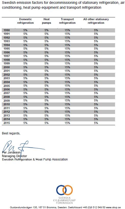
132 132

133 133

134 134