Development of a lab-scale auger reactor for biomass fast pyrolysis and process optimization using response surface methodology

Transcription

1 Graduate Theses and Dissertations Graduate College 2009 Development of a lab-scale auger reactor for biomass fast pyrolysis and process optimization using response surface methodology Jared Nathaniel Brown Iowa State University Follow this and additional works at: Part of the Mechanical Engineering Commons Recommended Citation Brown, Jared Nathaniel, "Development of a lab-scale auger reactor for biomass fast pyrolysis and process optimization using response surface methodology" (2009). Graduate Theses and Dissertations This Thesis is brought to you for free and open access by the Graduate College at Iowa State University Digital Repository. It has been accepted for inclusion in Graduate Theses and Dissertations by an authorized administrator of Iowa State University Digital Repository. For more information, please contact digirep@iastate.edu.

2 Development of a lab-scale auger reactor for biomass fast pyrolysis and process optimization using response surface methodology by Jared Nathaniel Brown A thesis submitted to the graduate faculty in partial fulfillment of the requirements for the degree of MASTER OF SCIENCE Co-Majors: Mechanical Engineering; Biorenewable Resources and Technology Program of Study Committee: Robert C. Brown, Major Professor Theodore J. Heindel D. Raj Raman Iowa State University Ames, Iowa 2009 Copyright Jared Nathaniel Brown, All rights reserved.

3 ii DEDICATION With gratitude and appreciation, this thesis is dedicated to my wife, Pari. Her love, support and understanding helped make this project possible.

4 iii TABLE OF CONTENTS LIST OF TABLES LIST OF FIGURES ABSTRACT v vii xi CHAPTER 1. INTRODUCTION Biomass fast pyrolysis Thesis overview 2 CHAPTER 2. TECHNICAL LITERATURE REVIEW Introduction Fast pyrolysis fundamentals Operating conditions End products description End product utilization Systems technology State of the art for auger type reactors Fossil fuel processing Biomass processing 26 CHAPTER 3. EXPERIMENTAL APPARATUS Lab-scale system design Lab-scale system components Lab-scale system development 62 CHAPTER 4. EXPERIMENTAL METHODS AND MATERIALS Introduction Experimental design 4.3 Experimental materials Testing procedures Product distribution Product analysis Data analysis and hypothesis testing 91 CHAPTER 5. RESULTS AND DISCUSSION Introduction Product distribution results Product analysis results 123 CHAPTER 6. CONCLUSIONS Research conclusions Regression models Product analysis Recommendations for future work 172 APPENDIX A. DESIGN AND DEVELOPMENT 175

5 iv APPENDIX B. MIXING STUDY 188 APPENDIX C. AUXILLARY EQUIPMENT AND INSTRUMENTS 194 APPENDIX D. EXPERIMENTAL DATA 200 REFERENCES 242 ACKNOWLEDGEMENTS 248

6 v LIST OF TABLES Table 1. Typical physical properties for bio-oil 9 Table 2. Comparison of auger reactor published data 35 Table 3. Biomass feeding system descriptions 50 Table 4. Heat carrier system descriptions 53 Table 5. Reactor system descriptions 56 Table 6. Product recovery system descriptions 59 Table 7. Shakedown trials operating conditions 65 Table 8. Factor considerations for experimental design procedure 68 Table 9. Selected factors and levels for experimental design 70 Table 10. Final central composite design, coded experiments 71 Table 11. Final central composite design, actual experiments 72 Table 12. Red oak biomass composition 73 Table 13. Red oak biomass ultimate and proximate analyses 74 Table 14. Steel shot composition and select properties 75 Table 15. Experimental operating conditions 76 Table 16. Description of symbols used in mass balance procedure 78 Table 17. Gas rotometer settings for experiments 79 Table 18. Non-condensable gas analysis for Run #24 83 Table 19. Thermal gravimetric analysis program method 88 Table 20. Chemical compounds quantified by GC/MS analysis 90 Table 21. ANOVA table 92 Table 22. Critical F-values for ANOVA F-test 93 Table 23. Lack of fit table 93 Table 24. Critical F-values for lack of fit F-test 94 Table 25. Critical t-values for t-test 96 Table 26. Summary of hypothesis tests 97 Table 27. Regression model coefficients and terms 98 Table 28. Sample experimental conditions for 8 selected tests 100 Table 29. Sample mass balance data for 8 selected tests 100 Table 30. Bio-oil yield model, statistics summary 103 Table 31. Biochar yield model, statistics summary 111 Table 32. Carbon monoxide yield model, statistics summary 119 Table 33. Carbon dioxide yield model, statistics summary 121 Table 34. Bio-oil moisture content model, statistics summary 127 Table 35. Water insoluble content model, statistics summary 132 Table 36. Ultimate analysis for biochar at center point tests 138 Table 37. Bio-oil carbon content model, statistics summary 144 Table 38. Bio-oil hydrogen content model, statistics summary 145 Table 39. Bio-oil oxygen content model, statistics summary 147 Table 40. GC/MS characterized compound comparison, whole bio-oil 156 Table 41. Reaction temperature model, statistics summary 162 Table 42. Regression models, summary of statistics 165 Table 43. Regression models, summary of significant terms 166 Table 44. Bio-oil analysis summary and comparison 167 Table 45. Motor power requirements analysis 181

7 vi Table 46. Shakedown trial operating conditions 186 Table 47. Shakedown trial yield and operating condition results 187 Table 48. Baseline biomass and sand mixture densities analytical data 192 Table 49. Biomass and sand mixture densities analytical data 193 Table 50. Feedstock and experimental condition data 200 Table 51. Product distribution and mass balance data 201 Table 52. Heat carrier system temperature data and other operating conditions 202 Table 53. Reactor system temperature data 203 Table 54. Product recovery system temperature data 204 Table 55. Bio-oil fraction mass balance data 205 Table 56. Bio-oil yield model statistical data 206 Table 57. Coded levels for model equations 207 Table 58. Biochar yield model statistical data 208 Table 59. Non-condensable gas yield model, statistics summary 209 Table 60. Non-condensable gas yield model statistical data 210 Table 61. Non-condensable gas data, composition 211 Table 62. Non-condensable gas data, molar analysis 212 Table 63. Non-condensable gas data, mass analysis 213 Table 64. Non-condensable gas data, volume meter properties 214 Table 65. Carbon monoxide yield model statistical data 215 Table 66. Carbon dioxide yield model statistical data 216 Table 67. Moisture content analytical data 217 Table 68. Moisture content model statistical data 218 Table 69. Water insoluble content analytical data 219 Table 70. Water insoluble content model statistical data 220 Table 71. Solids content analytical data 221 Table 72. Higher heating value analytical data 221 Table 73. Thermal Gravimetric Analysis data, bio-oil 221 Table 74. Thermal Gravimetric Analysis data, biochar 222 Table 75. Elemental analysis data, biochar 223 Table 76. Elemental analysis data, SF1 bio-oil 224 Table 77. Elemental analysis data, SF2 bio-oil 225 Table 78. Elemental analysis data, SF3 bio-oil 226 Table 79. Elemental analysis data, SF4 bio-oil 227 Table 80. Elemental analysis data, whole bio-oil 228 Table 81. Bio-oil carbon content model statistical data 229 Table 82. Bio-oil hydrogen content model statistical data 230 Table 83. Bio-oil oxygen content model statistical data 232 Table 84. Total acid number analytical data for center point tests 232 Table 85. GC/MS sample analytical data, Run #20 (maximum bio-oil yield) 234 Table 86. GC/MS analytical data, SF1 summary 235 Table 87. GC/MS analytical data, SF2 summary 236 Table 88. GC/MS analytical data, SF3 summary 237 Table 89. GC/MS analytical data, SF4 summary 238 Table 90. GC/MS analytical data, whole bio-oil summary 239 Table 91. Viscosity analytical data 240 Table 92. Reaction temperature model statistical data 241

8 vii LIST OF FIGURES Figure 1. Biomass fast pyrolysis schematic 2 Figure 2. Thermochemical processes 5 Figure 3. Fast pyrolysis product applications 12 Figure 4. Fast pyrolysis subsystem schematic 13 Figure 5. Biomass pretreatment schematic 13 Figure 6. Bio-oil recovery schematic 14 Figure 7. Bubbling fluidized bed reactor schematic 15 Figure 8. Circulating fluidized bed reactor schematic 16 Figure 9. Rotating cone reactor schematic 17 Figure 10. Auger reactor schematic, configuration 1 18 Figure 11. Auger reactor schematic, configuration 2 19 Figure 12. Ablative reactor concept 20 Figure 13. Hayes Process reactor 22 Figure 14. Lugi-Ruhrgas process schematic 23 Figure 15. Screw reactor concept 27 Figure 16. Twin screw mixer-reactor schematic 29 Figure 17. FZK twin screw mixer-reactor 29 Figure 18. Mississippi State University lab-scale auger reactor 32 Figure 19. University of Georgia auger reactor schematic 35 Figure 20. Lab-scale auger reactor system 39 Figure 21. Reactor design schematic 40 Figure 22. Heat carrier mass feed rates as a function of temperature change 42 Figure 23. Various auger flighting designs 43 Figure 24. Volumetric feed rate as a function of screw size and speed 44 Figure 25. Volumetric feed rate as a function of screw speed and configuration 45 Figure 26. Reactor lid drawing with dimensions in inches 46 Figure 27. Auger reactor rendering with lid removed 47 Figure 28. Auger reactor system rendering 48 Figure 29. Biomass feeding system schematic 49 Figure 30. Heat carrier auger drawing with dimensions in inches 51 Figure 31. Heat carrier system schematic 52 Figure 32. Reactor auger drawing with dimensions in inches 54 Figure 33. Reactor system schematic 55 Figure 34. Product recovery system schematic 58 Figure 35. LabVIEW program screenshot for data acquisition and process monitoring 61 Figure 36. Cold flow mixing images of cornstover biomass and silica sand 64 Figure 37. Corn stover (1.0 mm), corn fiber (1.0 mm) and red oak biomass (0.75 mm) 65 Figure 38. Sand, silicon carbide, alumina ceramic and steel shot heat carrier examples 65 Figure 39. Simplified reactor schematic with operational parameters shown 66 Figure 40. Central Composite Design schematic for two factors 69 Figure 41. Red oak biomass samples of three different grind sizes 73 Figure 42. SAE J827 steel shot size distribution 75 Figure 43. Reactor system schematic showing mass balance 77 Figure 44. Mass balance worksheet for experiments 80 Figure 45. Micro-GC gas analysis profile for Run #24 82

9 viii Figure 46. Temperature profile example for Run #20 84 Figure 47. Typical bio-oil recovery system temperatures 84 Figure 48. Product distribution results for the 30 fast pyrolysis tests 100 Figure 49. Pyrolysis product distribution range 101 Figure 50. Average operating temperature schematic for 6 center point runs 102 Figure 51. Bio-oil fraction distributions for 6 center point tests and for all tests 102 Figure 52. Absolute values for t-test statistics for bio-oil yield model 105 Figure 53. Actual vs. predicted bio-oil yield 105 Figure 54. Three response surfaces for modeled bio-oil yield 107 Figure 55. Modeled bio-oil yield as a function of heat carrier temperature and auger speed 109 Figure 56. Modeled bio-oil yield as a function of heat carrier temperature and feed rate 109 Figure 57. Absolute values for t-test statistics for biochar yield model 112 Figure 58. Actual vs. predicted biochar yield 112 Figure 59. Two response surfaces for modeled biochar yield 113 Figure 60. Modeled biochar yield as a function of heat carrier temperature and feed rate 115 Figure 61. Modeled biochar yield as a function of heat carrier temperature and auger speed 115 Figure 62. Average non-condensable gas composition at center points 117 Figure 63. Carbon monoxide and carbon dioxide yields vs. bio-oil yield for all tests 118 Figure 64. Actual vs. predicted carbon monoxide yield 120 Figure 65. Gas yields for 4 different species vs. bio-oil yield for all tests 122 Figure 66. Total non-condensable gas yield vs. bio-oil yield for 29 tests 122 Figure 67. Typical appearance of bio-oil fractions 123 Figure 68. Bio-oil moisture content at center points 124 Figure 69. Bio-oil moisture content range 124 Figure 70. Bio-oil moisture content vs. bio-oil yield for all tests 125 Figure 71. Absolute values for t-test statistics for moisture content model 127 Figure 72. Actual vs. predicted moisture content 128 Figure 73. Response surface for modeled moisture content 128 Figure 74. Modeled moisture content as a function of heat carrier temperature and auger speed 129 Figure 75. Water insoluble content for center points 130 Figure 76. Water insoluble content range 131 Figure 77. Modeled H 2 O insoluble content as a function of heat carrier temperature and feed rate 133 Figure 78. Water insoluble content vs. bio-oil yield for all tests 133 Figure 79. Actual vs. predicted water insoluble content 134 Figure 80. Solids content for center point tests 135 Figure 81. Higher heating value range 136 Figure 82. Biochar proximate analysis for center point tests 137 Figure 83. Bio-oil carbon content for center points 139 Figure 84. Bio-oil nitrogen content for center points 140 Figure 85. Bio-oil hydrogen content for center points 140 Figure 86. Bio-oil sulfur content for center points 141 Figure 87. Bio-oil ash content for center points 142 Figure 88. Bio-oil oxygen content for center points 143 Figure 89. Modeled bio-oil H content as a function of heat carrier temperature and feed rate 146 Figure 90. Actual vs. predicted oxygen content 147 Figure 91. Biochar and non-condensable gas yield vs. bio-oil yield for 29 tests 149 Figure 92. Bio-oil C, O, H, H 2 O and water insoluble contents as a function of yield for 30 tests 149 Figure 93. Bio-oil H:C ratio vs. O:C ratio (Van Krevelen diagram) for all 30 tests 150 Figure 94. C, O, H, H 2 O and H 2 O insoluble contents as a function of yield for 30 tests, dry basis 151

10 ix Figure 95. Bio-oil H:C ratio vs. O:C ratio for all 30 tests, including dry basis analysis 152 Figure 96. Total acid number for center points 153 Figure 97. GC/MS chromatogram for SF1, Run #20 (bio-oil max yield) 154 Figure 98. GC/MS chromatogram for SF4, Run #20 (bio-oil max yield) 155 Figure 99. GC/MS quantified volatile compounds 157 Figure 100. GC/MS quantified volatile compounds by fraction for center points 158 Figure 101. Viscosity measurements for Run #20 vs. time 159 Figure 102. Bio-oil viscosity range 160 Figure 103. Reaction temperature schematic 161 Figure 104. Vapor temperatures vs. heat carrier temperatures 161 Figure 105. Actual vs. predicted reaction temperature 163 Figure 106. Absolute values for t-test statistics for vapor temperature model 164 Figure 107. Modeled vapor temperature vs. heat carrier temperature 165 Figure 108. Recommended system design modifications 173 Figure 109. Heat carrier residence time as a function of auger speed 180 Figure 110. Biomass feeding system 182 Figure 111. Close-up of reactor augers 182 Figure 112. Reactor mounted on frame 182 Figure 113. Reactor lid and thermocouple detail 183 Figure 114. Gas cyclone 183 Figure 115. Condensers 1 and 2 (SF1 and SF2) 183 Figure 116. Electrostatic precipitator (SF3) 184 Figure 117. Condenser 3 in ice bath (SF4) 184 Figure 118. Reactor system detail 185 Figure 119. Biomass and sand mixture densities 188 Figure 120. Mixture density (L) vs. auger speed at three axial locations, Run Figure 121. Mixture density (L) vs. auger speed at three axial locations, Run Figure 122. Mixture density (C) vs. auger speed at four axial locations, Run Figure 123. Pentapycnometer instrument 191 Figure 124. Mixture density (C) vs. auger speed at four axial locations, Run Figure 125. Hammer mill 194 Figure 126. Knife mill 194 Figure 127. CHN/O/S analyzers 195 Figure 128. Thermal gravimetric analyzer 195 Figure 129. Bomb calorimeter 196 Figure 130. Moisture analyzer 196 Figure 131. Micro-GC cart 197 Figure 132. Gas volume meter and pressure gauge 197 Figure 133. Moisture titrator 198 Figure 134. Total acid number titrator 198 Figure 135. GC/MS 199 Figure 136. Viscometer 199 Figure 137. Residuals for bio-oil yield full model 206 Figure 138. Residuals for biochar yield full model 208 Figure 139. Residuals for non-condensable gas yield full model 209 Figure 140. Residuals for carbon monoxide yield full model 215 Figure 141. Residuals for carbon dioxide yield full model 216 Figure 142. Residuals for moisture content full model 218 Figure 143. Residuals for water insoluble content full model 220

11 x Figure 144. Residuals for bio-oil carbon content full model 229 Figure 145. Residuals for bio-oil hydrogen content full model 230 Figure 146. Predicted vs. actual hydrogen content 231 Figure 147. Residuals for bio-oil oxygen content full model 231 Figure 148. GC/MS chromatogram for SF2, Run #20 (bio-oil maximum yield) 233 Figure 149. GC/MS chromatogram for SF3, Run #20 (bio-oil maximum yield) 233 Figure 150. Quantified mass for all runs 240 Figure 151. Residuals for reaction temperature full model 241

12 xi ABSTRACT A lab-scale biomass fast pyrolysis system was designed and constructed based on an auger reactor concept. The design features two intermeshing augers that mix biomass with a heated bulk solid material that serves as a heat transfer medium. A literature review, engineering design process, and shake-down testing procedure was included as part of the system development. A response surface methodology was carried out by performing 30 experiments based on a four factor, five level central composite design to evaluate and optimize the system. The factors investigated were: (1) heat carrier inlet temperature, (2) heat carrier mass feed rate, (3) rotational speed of the reactor augers, and (4) volumetric flow rate of nitrogen used as a carrier gas. Red oak (Quercus Rubra L.) was used as the biomass feedstock, and S-280 cast steel shot was used as a heat carrier. Gravimetric methods were used to determine the mass yields of the fast pyrolysis products. Linear regression methods were used to develop statistically significant quadratic models to estimate and investigate the bio-oil and biochar yield. The optimal conditions that were found to maximize bio-oil yield and minimize biochar yield are high nitrogen flow rates (3.5 sl/min), high heat carrier temperatures (625 C), high auger speeds (63 RPM) and high heat carrier feed rates (18 kg/hr). The produced bio-oil, biochar and gas samples were subjected to multiple analytical tests to characterize the physical properties and chemical composition. These included determination of biooil moisture content, solid particulate matter, water insoluble content, higher heating value, viscosity, total acid number, proximate and ultimate analyses and GC/MS characterization. Statistically significant linear regression models were developed to predict the yield of gaseous carbon monoxide, the hydrogen content, moisture content and water-insoluble content of the bio-oil, and the vapor reaction temperature at the reactor outlet. A significant result is that with increasing bio-oil yield, the oxygen to carbon ratio and the hydrogen to carbon ratio of the wet bio-oil both decrease, largely due to a reduction in water content. The auger type reactor is currently less researched than other systems, and the results from this study suggest the design is well suited for fast pyrolysis processing. The reactor as designed and operated is able to achieve high liquid yields (greater than 70%-wt.), and produces bio-oil and biochar products that are physically and chemically similar to products from other fast pyrolysis reactors.

13 1 CHAPTER 1. INTRODUCTION A fundamental branch of the mechanical engineering discipline is energy conversion, transforming naturally occurring resources into forms that are more usable by society. Energy conversion is an application of engineering principles from thermodynamics, fluid mechanics, and heat transfer, as well as machine design and mechanics of materials. A classic example of an energy conversion process is coal combustion to provide heat for raising steam that runs turbines and generators for producing electricity. More recently, however, biomass has been recognized as a viable and abundant resource that can be used for the production of renewable fuels, energy, chemicals and other bioproducts [1]. According to The Global Summit on the Future of Mechanical Engineering 2028, One of the most critical challenges facing mechanical engineers is to develop solutions that foster a cleaner, healthier, safer and sustainable world [2]. Biomass fast pyrolysis is an energy conversion process that can be considered one such solution to these challenges. The objective of this research study is to design and develop a novel lab-scale auger reactor for biomass fast pyrolysis processing, determine its optimal operating conditions, and relate the product yields and composition to these conditions. This will allow for the reactor design to be evaluated and compared to existing, published data. This reactor type is relatively new in the field of biomass fast pyrolysis, and can be currently considered as an alternative reactor. Though there are potential economic and processing advantages of utilizing this reactor technology for bio-oil production, there is little published data relating the pyrolysis product yields and composition to the operating conditions of the reactor. 1.1 Biomass fast pyrolysis Fast pyrolysis is a thermochemical process used to produce primarily a liquid product known as pyrolysis oil or bio-oil [3], and is considered a promising route for biomass conversion. When biomass is rapidly heated in a controlled, oxygen depleted environment at atmospheric pressure to a final temperature of approximately 500 C, it is decomposed and converted within seconds to liquid bio-oil, solid biochar, and non-condensable gases [4]. Fast pyrolysis can collect over 70% of the starting material mass as liquid bio-oil, with the balance formed by approximately equal portions of biochar and gases.

14 2 Bio-oil can be used as a renewable industrial fuel to generate heat and electrical power, or can be upgraded into transportation fuels and specialty chemicals. Biochar can be used as a solid fuel source, and has more recently found applications as an agricultural soil amendment. The noncondensable gases are typically recycled into the process to provide process heat. A general schematic of this thermal process is shown in Figure 1, noting the relationship between the fast pyrolysis reactor and the system that separates and collects the reaction products. Also note the energy input to the reactor in the form of heat, which is required to carry out the endothermic fast pyrolysis reactions. Figure 1. Biomass fast pyrolysis schematic 1.2 Thesis overview This thesis consists of five remaining sections to systematically explain and support the research effort. The next section, Chapter 2, will summarize the literature review performed to determine the general state-of-the-art of the science and technology of biomass fast pyrolysis and review previous research efforts related to auger reactors. Chapter 3 will review the R&D efforts required to construct the laboratory reactor system, including a detailed description of the apparatus. Chapter 4 will detail the methodology and materials used for the experimental phase of the research. The results of the experiments will be presented in Chapter 5 along with a discussion, and Chapter 6 includes the conclusions of the research and recommendations for future work. Supplemental information is located in Appendices and will be referred to as necessary.

15 3 CHAPTER 2. TECHNICAL LITERATURE REVIEW 2.1 Introduction Lignocellulosic biomass is an abundant and geographically diverse natural resource. The USDA estimates that over one billion tons of dry matter may be available annually in the United States [5]. Examples of biomass resources include: agricultural crop residues such as corn stover, wood residues from the forest and milling industries, municipal solid waste (MSW) from urban areas, herbaceous energy crops such as switchgrass, and short-rotation woody crops [6]. Through photosynthesis, plants convert sunlight and CO 2 into stored chemical energy, therefore biomass can be considered an indirect form of solar energy and a renewable source of carbon [7]. The stored chemical energy in biomass can be converted into bioenergy (heat and electricity), liquid biofuels for transportation, chemicals, and other biobased products. This utilization of biomass can contribute to a net reduction in greenhouse gas emissions which may impact global climate change, and provide other benefits such as reducing foreign energy imports [8]. There are many biomass conversion pathways in various stages of development, and these pathways are commonly grouped into two major technology platforms: biochemical and thermochemical. These platforms are not exclusive, though, and opportunities exist to combine technologies into so-called hybrid processes [9]. Biochemical technologies, such as fermentation to produce alcohol fuels and anaerobic digestion to produce methane gas, are outside the scope of this research and will not be discussed. Thermochemical conversion techniques utilize heat to decompose biomass, and include four main processes (in order of increasing temperature): direct liquefaction, pyrolysis, gasification and combustion. Though pyrolysis and liquefaction are sometime grouped into one process, they will be discussed here separately. Direct liquefaction. Direct liquefaction, or often just liquefaction, is a mild temperature, high pressure conversion process (around 300 C and up to 240 bar, respectively) with the primary goal of producing a liquid product [1]. Liquefaction is often a catalytic process, and requires that the feedstock material be slurried in an aqueous solution, usually with water as a solvent. Because of this requirement, liquefaction may be well suited for resources that naturally have particularly high moisture contents, such as animal manure. Huber et al. [10] note that while bio-oils from liquefaction (often referred to as bio-crude) are of a high quality due to the low oxygen content, this comes at the

16 4 expense of a lower liquid yield. In general, direct liquefaction has been less investigated than other thermochemical processes; however refer to Behrendt et al. [11] for a recent review of direct liquefaction. Applications of bio-crude are similar to applications for bio-oil, and will be discussed later. Pyrolysis. Pyrolysis is the thermal decomposition of organic matter without oxygen present [3]. The origins of pyrolysis date back as far as ancient Egypt [4]. Upon heating, moisture is first driven off from a material, and then pyrolysis reactions occur before any remaining thermal processes occur. Depending on the conditions, varying amounts of solid, liquid and gas will be produced [12]. Pyrolysis occurs over a range of temperatures from 400 C 600 C, and usually at atmospheric pressure. Fast pyrolysis is marked by high heating rates, short vapor residence times (seconds) and rapid cooling of the reaction products, which favors maximum formation of liquids around 500 C [13]. Slow pyrolysis, alternatively, is marked by slower heating rates, longer vapor residence times (minutes), and high yields of solid char material [4]. Slow pyrolysis also known as conventional pyrolysis has basically been applied for many years as a carbonization type process for converting wood into charcoal [4, 14]. As slow pyrolysis yields minimal bio-oil, it will not be reviewed further. In addition to fast and slow pyrolysis (which are not always clearly delineated), several other types of pyrolysis are reviewed by Mohan et al. [4]. The fast pyrolysis process and technology, including applications for the end-products, are discussed in more depth in the next section. A benefit of direct liquefaction and pyrolysis over gasification and combustion is the ability to produce a liquid product, which can be more readily stored and transported compared to gaseous fuels. This implies that bio-oil can be produced in a separate location from the end-use application, and this distributed processing scheme may be advantageous as biomass transportation costs can be minimized for small scale regional facilities [15]. Gasification. Gasification is an endothermic process occurring around process temperatures of 750 C 1000 C to produce primarily a combustible fuel gas commonly referred to as producer gas or syngas [1]. Depending on the process conditions and the fluidizing gas, the syngas composition will contain varying amounts of CO, H 2, CH 4, CO 2, N 2 and other organic species. The heat required for gasification is often provided by partially oxidizing a portion of the feedstock material. Syngas can be combusted for heat and power applications, or upgraded into transportation fuels and chemicals using the Fischer-Tropsch process or other techniques [16]. For more information on gasification technology refer to Ciferno et al [17]. Combustion. Combustion is the highest temperature thermochemical conversion process (in excess of 1500 C), and it is well understood and commonly used in many industries. With

17 5 stochiometric or excess air present to fully oxidize the feedstock fuel, combustion produces heat with water and CO 2 as byproducts. Heat from combustion is used for various processes, including steam production and electricity generation. This process will not be reviewed further, however refer to Jenkins et al. for more information on biomass combustion [18]. Refer to Demirbas for a thorough review of thermal conversion of biomass [19], and Olofsson et al. for a review of applicable technologies and reactor configurations [20]. An overview of these processes and their general applications is shown in Figure 2. Liquefaction is shown offset in Figure 2 because it is not as well researched as the other thermochemical processes, and is sometimes not even mentioned as a thermal process and lumped together with pyrolysis as a means for producing primarily liquid fuels. LIQUEFACTION LIQUID CHEMICALS PYROLYSIS SOLID UPGRADING FUELS GASIFICATION GAS POWER COMBUSTION HEAT Figure 2. Thermochemical processes 2.2 Fast pyrolysis fundamentals Fast pyrolysis is a complex process, and though much research has been performed over the past few decades, it is still developing at a rapid rate. This process has shown great promise for being flexible and diverse, and is prized for the ability to produce a high yielding liquid fuel from almost any type of biomass feedstock. Minimal biomass pretreatments are required for fast pyrolysis [3], and

18 6 depending on the desired outputs the process can be carried out such that no outside energy inputs are required. Furthermore, depending on the product applications, fast pyrolysis can be a carbon neutral or even carbon negative process. As previously noted, fast pyrolysis is a rapid heating process in the lack of oxygen to decompose biomass into a liquid fuel, with solid and gaseous by-products. It is generally accepted that there are four main process characteristics for fast pyrolysis [4, 21], and will be discussed in more depth in the next section: Very high heat transfer rates Controlled reaction temperature Short vapor residence times Rapid separation and cooling of reaction products As the fast pyrolysis process occurs in a few seconds or less, heat transfer and mass transfer effects as well as reaction kinetics are all important phenomenon, however these considerations will not be reviewed here and can be found elsewhere [22-27]. Blasi [28] and Babu [29] discuss several different kinetic models in separate reviews of biomass pyrolysis Operating conditions There is much literature reported on the operating conditions for biomass fast pyrolysis, and biomass properties are the first consideration in maximizing liquid yield. To ensure rapid heating and complete devolatilization, small biomass particles are required. Though the particle size requirement is somewhat dependent on the specific reactor technology used, the general particle size requirement is agreed to be around 2.0 mm [10, 21, 30]. The only other pretreatment required prior to fast pyrolysis is reduction of the biomass moisture content. Typical requirements are around 10%-wt. or less, which minimizes the amount of water that is collected in the final bio-oil [21] and decreases the overall reaction heat energy requirements. Overall fast pyrolysis is an endothermic process, with sensible heat required to bring the biomass from ambient conditions to the reaction temperature regime. Above the sensible heat requirements, though, the fast pyrolysis reactions require a minimal heat addition. Daugaard et al. estimate a total heat for pyrolysis ranging from MJ/kg depending on the feedstock [31]. The condition that this heat be rapidly transferred to the biomass is critical for fast pyrolysis, and many

19 7 mechanisms and reactor configurations have been researched and developed to accomplish this. Heating rates on the order of 10 3 C/sec have been claimed [4]. If biomass is slowly heated, secondary reactions occur and more solid products are formed as liquid yields are decreased [32]. Rapid heating in a fast pyrolysis reactor typically occurs by means of a hot carrier gas or solid heat carrier material, or a heated reactor wall, or a combination of these [21, 33]. Though the addition of air or oxygen can provide heat by oxidizing a portion of the feedstock (as is performed for biomass gasification), this approach decreases the yield of bio-oil. Therefore, many reactors (especially lab-scale systems for research purposes) utilize a flow of nitrogen gas to provide an inert reaction environment. Depending on the reactor configuration, the heat transfer mode of conduction, convection or radiation may dominate, however they will each contribute to some degree. The reaction temperature is also critical for fast pyrolysis and has effects on the product yields and qualities. Higher char formations occur at temperatures less than approximately 425 C, and non-condensable gas production increases for temperatures above 600 C. Several sources report bio-oil yields are maximized around temperatures of 500 C ± 25 C [4, 13, 21, 30]. The heat transfer rate and the reaction temperature are both important: rapid heating to a reaction temperature that is too low or too high will adversely affect the products, as will a slow heating rate to the optimal reaction temperature. The reaction pressure for fast pyrolysis is typically near atmospheric, as higher pressures favor the formation of biochar [34]. In addition to rapid heating and controlled temperatures, a short residence time for the pyrolysis products is important to maximize liquid yields. As biomass is pyrolyzed, the reaction products evolve in the form of condensable vapors, tiny aerosol droplets, non-condensable gases and biochar. From the time biomass enters the reactor, the vapor residence time (where vapors here are considered to be all the reaction products other than solid biochar particles) is traditionally less than 2 seconds for fast pyrolysis. This consideration is extended to include the cooling of the vapor and aerosol products to collect them as bio-oil. For instance if the reaction products are formed in the reactor within the first second, within the next second they should be rapidly cooled to condense and recover as much vapors and aerosols as possible. The cooling process during the collection of bio-oil effectively minimizes further reactions that occur at high temperatures, so fast pyrolysis can not be considered an equilibrium process [4]. As with the optimal reaction temperature for fast pyrolysis, the 2 second vapor residence time is currently a well accepted and documented operating condition [4, 13, 30]. Longer residence times allow for secondary reactions to occur which form either additional gases or char, both of which are undesired and reduce the liquid yield.

20 End products description The chemical and physical characteristics of the fast pyrolysis products are dependent on many factors, including: the biomass composition and the operating conditions (as discussed previously), as well as the reactor and product recovery technology used for the processing (as discussed in Section 2.2.4). A brief introduction to the products of fast pyrolysis is presented next. Bio-oil. The primary product from fast pyrolysis is a dark brown liquid known as pyrolysis oil, bio-oil, liquid smoke, wood distillate, or a number of many other terms. Bio-oil has a distinct odor similar to smoke from a wood fire, and is often quite pungent. As discussed, the yield of bio-oil will vary depending on the operating conditions and feedstock properties, but yields in excess of 70%-wt. are common for wood biomass and well documented in the literature. In general, bio-oil yields for biomass fast pyrolysis range from 65%-wt. 75%-wt. Bio-oil is a complex mixture of more than 300 organic compounds formed during pyrolysis reactions that are essentially trapped in a liquid form [35]. Bio-oil is very different from traditional fossil-fuel based liquids, and indeed some researchers prefer not to refer to it as oil at all ( pyrolysis liquid, for example). Many of these differences and the unique properties of bio-oil are attributed to its high oxygen content (over 40%-wt.), which originates from the oxygen contained in the biomass feedstock. It is often noted that bio-oil elemental composition is very similar to that of the original feedstock, just in a more convenient liquid form [4, 36]. Bio-oil also contains significant amounts of water, which results from condensing any moisture contained in the feedstock as well as significant reaction water formed during the process. A common value for bio-oil moisture content is 25%-wt. An important aspect of bio-oil is that it can not be directly mixed with hydrocarbon fuels because phase separation occurs due to the high moisture content. Also due to the high oxygen and water contents, bio-oil has a lower heating value than petroleum based fuel-oils, often reported around 40% 50% less [4, 36]. In addition to higher oxygen and water contents, bio-oil is more acidic than petroleum based fuel-oils, with a common ph value of 2.5. Common physical properties of bio-oil are shown in Table 1, as reported by the reviewed literature. Note that bio-oil cannot be readily heated for distillation purposes. Due to its unique nature, a residue of up to 50%-wt. may remain. This has implications for bio-oil upgrading operations, which are discussed in the next section. The chemical composition of bio-oil is dependent on many factors, and includes many classes of oxygenated species. In addition to water, Bridgwater et al. describe the major chemical constituents of bio-oil as: aldehydes (15%-wt.), carboxylic acids (12%-wt.), carbohydrates (8%-wt.), phenols (3%- wt.), furfurals (2%-wt.), alcohols (3%-wt.) and ketones (3%-wt.) [13]. Alternatively, Mohan et al. list

21 9 five more general categories of chemical compounds: hydroxyaldehydes, hydroxyketones, sugars and dehydrogugars, and phenolic compounds [4]. Another major constituent of bio-oil (15%-wt. 30%- wt.) is a water-insoluble fraction thought to originate from the lignin portion of the biomass, and is therefore often referred to as pyrolytic lignin [4, 13]. Some of the interesting properties of bio-oil are based on the pyrolytic lignin fraction, as are the processing challenges and opportunities associated with bio-oil. Table 1. Typical physical properties for bio-oil Property Water content Specific gravity Viscosity ph Heating value Solids content Elemental analysis Unit Value Notes %-wt Wet basis cp 40 C MJ/kg HHV %-wt Wet basis %-wt. Wet basis Carbon Hydrogen Oxygen Nitrogen Ash Distillation residue %-wt. ~50 Wet basis Note: Adapted from [10, 21, 36-38]. Refer to these sources for more in-depth reviews of bio-oil physical properties. Though the chemical and physical characterization of bio-oil has been researched for decades, methodologies and standards are still being developed. Specific methodologies and practices important to this research will be discussed as necessary in later sections. Refer to Oasmaa et al. for several studies of commonly used procedures and recommendations for bio-oil testing [38-40]. Bio-oil has unique aging and stability issues, and as it is not an equilibrium reaction product it is known to change over time. Low temperature storage is a commonly used practice to minimize these changes. Bio-oil stability will not be discussed here, but is documented in the literature and is currently a research topic of great interest. Non-condensable gas. The gaseous products from fast pyrolysis will be referred to as noncondensable gas (NCG), rather than syngas or producer gas which is reserved for the reaction products of gasification. The NCG fraction from fast pyrolysis is a combustible mixture, and contains many species including: large amounts of carbon monoxide (CO) and carbon dioxide (CO 2 ), with

22 10 lesser amounts of hydrogen (H 2 ), methane (CH 4 ), ethylene (C 2 H 4 ), ethane (C 2 H 6 ), propane (C 3 H 8 ), and other light hydrocarbons. The NCG stream will also contain any un-reactive gases that were used in the process for fluidization, such as nitrogen. As with bio-oil and biochar, the NCG yield and composition will be dependent on many factors including the process conditions and feedstock. NCG yield is in the range of 10%-wt. to 20%-wt, and commonly has a yield similar to that of biochar. Biochar. The solid product from fast pyrolysis is a black, powdery substance known as biochar, char, agri-char or just charcoal [41]. Biochar yields from fast pyrolysis range from approximately 11%-wt. to around 25%-wt., with 13%-wt. to 15%-wt. being common values for fast pyrolysis of wood biomass. Elementally, biochar is composed mostly of carbon (> 60%-wt.), with smaller amounts of hydrogen, oxygen, nitrogen and sulfur depending on the biomass composition. In 2007, Mohan et al. reported biochar with fixed carbon values up to 78%-wt. and higher heating values up to 31.7 MJ/kg [42]. Typically the majority of the ash component in the biomass feedstock ends up concentrated in the biochar. The physical, chemical and biological properties of biochar vary widely, and are reviewed in a recent and comprehensive book by Lehmann & Joseph [41] End product utilization Bio-oil. There are many applications for bio-oil, in varying stages of research and commercial implementation. As produced, bio-oil can be considered a fuel source for standard industrial equipment such as boilers, furnaces, burners, stationary diesel engines, gas turbines and stirling engines [4, 36, 43]. Bio-oil used for generating heat or electricity in these applications displaces the use of light fuel oil, heavy fuel-oil or even diesel fuel; however modifications are often required to accommodate the unique properties of bio-oil as discussed. In these applications, options exist to potentially emulsify or co-fire traditional fuels with bio-oil. Bio-oil used for heat and power applications have been demonstrated with documented decreases in certain emissions. Refer to Bridgwater et al. [13], Czernik et al. [36], and Oasmaa et al. [38] for more information. Gust et al. also review potential standards for bio-oil properties used in heat and power applications [44]. In addition to utilizing bio-oil directly, there are various options for bio-oil utilization that require an intermediate upgrading step. Recently there has been considerable research and commercial interest in upgrading bio-oil into synthetic hydrocarbon fuels for transportation applications. For this type of application, the high oxygen content of bio-oil is reduced through deoxygenation processes commonly used in the petrochemical industry: hydrotreating and catalytic cracking [10, 13, 21, 36]. These processes upgrade bio-oil at high temperatures and pressures with

23 11 hydrogen present. Refer to Jones et al. for a design study considering bio-oil as a feedstock for upgrading to diesel and gasoline [45], Huber et al. for a study of integrating bio-oil into petroleum refineries [46], and Elliot for a review of bio-oil upgrading [47]. A different approach to synthesizing transportation fuels from bio-oil is using the pyrolysis liquid as a feedstock for gasification, rather than raw biomass. By gasifying a slurry of bio-oil and biochar, it is possible to produce a clean syngas which is then upgraded to transportation fuels using Fischer-Tropsch processing [48]. A final upgrading consideration for bio-oil is using steam reforming techniques for the production of hydrogen [10, 35, 49]. Hydrogen is required for many industrial processes, is frequently used in the petrochemical industry, and can be used in fuel cells to generate electricity. Even though bio-oil is a complex liquid, is contains specific compounds such as acetic acid, levoglucosan, and hydroxyacetaldehyde that have been researched for potential extraction [36, 43]. There are many other specialty products originating from bio-oil that are already in commercial use or have been identified, including: wood preservatives, insecticides and fungicides, fertilizers, resins, adhesives, road de-icers and numerous food flavorings and additives [21, 36]. Non-condensable gas. The gaseous by-products of fast pyrolysis are of relatively low value; hence their main application is direct combustion to provide heat as part of the fast pyrolysis process. This use of the gas, rather than flaring or reserving for a different application, makes the process more thermally efficient and more greenhouse gas neutral because auxiliary fossil-fuel based sources are minimized. In lab-scale applications, the non-condensable gas is typically vented. Biochar. Until recently, biochar was often considered a fast pyrolysis by-product similar to the non-condensable gas in that its best use is as a fuel source to provide energy for the process. As biochar has a high carbon content, it is a relatively energetic material that can contribute heat energy for the reactions or biomass drying, thus minimizing external fuel inputs. More recently, however, there has been research interest in utilizing biochar as a soil amendment [41, 50]. In this approach, biochar is incorporated into the soil where the biomass was harvested from, which provides benefits to the soil, the crop and the environment including a net reduction in atmospheric carbon [51]. In this sense the biochar is referred to as a carbon sequestration agent, as shown in the schematic of fast pyrolysis (FP) applications in Figure 3.

24 12 Figure 3. Fast pyrolysis product applications Image adapted from Bridgwater et al. [21] Systems technology As with any advanced process, fast pyrolysis systems are composed of multiple subsystems. The generalized subsystems that will be discussed are: pretreatment, reactor, and product recovery with a relationship as shown in Figure 4. Pretreatment. Compared to other biomass conversion technologies, the so called pretreatment required for fast pyrolysis processing is minimal [30]. Typically no catalysts are used, and no chemical treatments are required. Typically only size reduction and drying are required. As shown in Figure 5, raw biomass from a storage and handling facility is passed through a chopping device to reduce the particle size of the biomass and homogenize it such that it can easily be transported through a dryer. Heat for drying purposes can be provided with either flue gas from a direct use combustor as shown, or with process heat originating elsewhere. Finally, a grinder or milling device is used to reduce the biomass particles to the desired size range, typically around 2 mm as discussed previously. This is a general pretreatment subsystem, and specific technologies related to drying and size reduction will not be discussed and can be found elsewhere.

25 13 Figure 4. Fast pyrolysis subsystem schematic Figure 5. Biomass pretreatment schematic Before specific reactor technologies are discussed, common biochar and bio-oil recovery technologies will be discussed. The biochar recovery and bio-oil recovery technologies combined represent the product recovery subsystem shown in Figure 4. These technologies are discussed first because very similar product recovery technologies are utilized on fast pyrolysis systems, largely independent of the reactor type. Biochar recovery. It is important that biochar is separated from the remaining pyrolysis products quickly because interactions with char may cause unwanted secondary reactions. For biochar collection and separation, gas cyclones are common and used frequently because of their simple design and operation [21]. Gas cyclones have no moving parts, are well understood and used successfully in many industrial applications. Though well researched and able to provide high collection efficiencies (above 99%), cyclone separators are not able to collect very fine particulate matter. This is true even when multiple cyclones are used in series [13]. Other biochar collection equipment such as hot vapor filtration and moving bed filters [52] have been researched and are still under development. As such, some biochar particles inevitably bypass biochar collection equipment and end up as fine particulate matter suspended in the collected bio-oil. This can be a problematic for

26 14 certain bio-oil utilization equipment or processes, whereas in other applications this may be advantageous because of the increased energy value associated with the biochar. The amount of biochar in bio-oil (reported on %-wt. basis) can be determined by addition of a solvent such as methanol because the biochar particles will not dissolve with the liquids and can be filtered out. Bio-oil recovery. As discussed, bio-oil recovery technology is crucial to quickly cool the reaction products so as high yields can be realized. The associated technology can be complex and varies greatly between systems, with major differences between lab-scale and commercial reactors. Many research sized fast pyrolysis systems use a staged approach to cool and collect the reaction products sequentially. Small systems typically use water and ice cooled condensers or impingers, and a 2002 study by Gerdes et al. reviews the design and construction of a common lab-scale setup [53]. In contrast to simple heat exchangers, a more traditional technology for larger scale systems is a quenching type device in which collected bio-oil is re-circulated and cooled before being sprayed onto a stream of hot vapors and aerosols exiting the reactor. This type of quenching process minimizes potential blockages in heat exchanger type condensers [13]. Bio-oil aerosols are particularly difficult to collect, and a secondary device in addition to the quench system is often required. Denoted as a filter in Figure 6, an electrostatic precipitator (ESP) is the preferred secondary collection technology [13, 21]. Non-condensable gas is effectively separated from the collected bio-oil in the quench system as shown. Figure 6. Bio-oil recovery schematic

27 15 Bubbling fluidized bed. Bubbling fluidized bed (BFB) reactors, or more simply fluidized beds or even just fluid beds, are commonly used for bio-oil production and data from these systems is widely published and available. Refer to Boateng et al. [54] for a recent representative study, and Bridgwater et al. [30] for a detailed review. These systems used for fast pyrolysis have been developed over decades, based on similar technology used for combustors in industries including petrochemical and manufacturing. A well recognized company in fast pyrolysis processing is Dynamotive Energy Systems (Canada), and several bubbling fluidized bed reactors operate commercially using their patented BioTherm process [55]. Refer to a review of short residence time cracking processes by Hulet et al. for details on the BioTherm process [56]. Referring to Figure 7, a feeding system is used to mechanically (or pneumatically) convey biomass into a vertical reactor vessel featuring a bed of hot sand. A large flow of inert gas is used to fluidize the sand, providing a well-mixed volume with excellent heat transfer characteristics in which the reactions occur. The reactor, in this example, is heated indirectly by combustion flue gas in an annulus around the reactor, where other heating provisions such as tubes through the reactor are possible [21]. Pyrolysis products, including condensable bio-oil vapors and aerosols, biochar and non-condensable gases exit the top of the reactor with the fluidizing gas. Biochar and bio-oil are then collected as discussed. Resulting non-condensable gases are recirculated as a fluidizing gas or can be combusted for process heat. Figure 7. Bubbling fluidized bed reactor schematic

28 16 Note that Figure 7 is only one representation of this reactor type, where modifications to the gas handling and reactor heating configurations are common. For instance, biochar is shown here to be a by-product, where instead it could be used as a fuel source for the combustor to limit the auxiliary fuel requirement. Details of the biomass pretreatment and bio-oil recovery operations can be found in Figure 5 and Figure 6, respectively, as discussed previously. Though fluidized beds have been demonstrated commercially and provide high liquid yields, heat transfer problems can be significant and significant energy can be required to handle the fluidizing gas. Circulating fluidized beds. Circulating fluidized bed (CFB) reactors, sometimes referred to as transport beds, are similar to bubbling fluidized beds. However rather than having bed material remain suspended in one reactor, CFBs have a separate combustion reactor used to re-heat the sand which is continuously recirculated. As with fluidized beds, the CFB reactor is well understood and is currently used in several industries on commercial scales. One configuration of a CFB reactor for fast pyrolysis is shown in Figure 8, noting that biochar entrained with the bed material is combusted in the presence of air to provide heat for the re-circulated sand. Another Canadian company, Ensyn, utilizes circulating fluidized bed reactors as part of their proprietary Rapid Thermal Processing (RTP) technique used at several commercial fast pyrolysis plants [57]. Through a partnership with Red Arrow, the RTP technique is used to produce a consumer grade food flavoring, which is often referred to as liquid smoke [58]. Figure 8. Circulating fluidized bed reactor schematic

29 17 The CFB design has similar advantages as the BFB and may have fewer problems scaling up, but the sand recirculation loop requires significant complexity. As such, the CFB is not a common reactor design used for lab-scale fast pyrolysis studies. Refer to Hulet et al. for a review of several configurations of the Ensyn RTP design [56]. Rotating Cone. The rotating cone reactor is quite different than the bubbling fluidized or circulating fluidized bed reactors [3]. Rather than a vertical reaction vessel with bed material that remains well-mixed due to flowing fluidization gas, biomass is mechanically mixed in a rotating cone with a bulk solid heat transfer medium. Sand is used as the heat transfer medium, and is referred to as a heat carrier. Though sand is used as a heat carrier material in the fluidized bed reactors, hot fluidizing gas is also used to promote heat transfer and mixing effects. Therefore, one benefit of the rotating cone reactor is minimizing the amount of gas required for the process. However, as shown in Figure 9, one configuration of the rotating cone reactor includes a separate fluidized bed reactor to combust the biochar to provide heat for the recirculated sand. This aspect of the rotating cone design is very similar to the operation of the CFB reactor. The rotating cone reactor concept has been commercialized through work by Biomass Technology Group (BTG) in the Netherlands, which has developed a 50 ton per day facility in Malaysia [59]. In this design, sand and biomass are driven up the wall of the cone due to fast rotation speeds from RPM, and pyrolysis products exit from the top of the cone [13, 21, 56]. COMBUSTOR & HX HOT SAND BIOCHAR PRODUCTS CYCLONES REACTOR Figure 9. Rotating cone reactor schematic

30 18 Though the BTG rotating cone concept has claimed high liquid yields from a physically compact system [59], it has not been proven at large scales or operated for significant time periods. Auger reactor. The auger reactor concept also features mechanical mixing of biomass and a bulk solid heat transfer medium. However instead of the reactor vessel itself rotating, there are mixing devices that rotate inside a stationary horizontal reaction vessel. Typically the biomass and heat carrier are independently metered into the reactor, and the heat carrier is heated prior before entering the reactor. Figure 10 shows a reactor with two augers (or screws); however a single auger or similar mechanical mixing implement may also be used. As vapor products evolve they exit the reactor due to pressure differences, and the solid materials including biochar and the heat carrier exit at the end of the reactor. Similar to the previous designs, some biochar does leave the auger reactor with the vapor products and is removed with cyclones as discussed previously. A solid separator device can be used to remove biochar from the heat carrier material based on differences in particle size or density. Similar to CFB and rotating cone reactors, a combined heat exchanger and combustion reactor then reheats the heat carrier before it is recirculated into the auger reactor. Figure 10. Auger reactor schematic, configuration 1 Alternatively, Figure 11 shows an auger reactor that does not separate the biochar from the heat carrier. Similar to the CFB reactor, biochar is combusted to reheat the recirculated heat carrier.

31 19 BIOMASS PRE TREATMENT PRODUCTS AUGER REACTOR BIO-OIL RECOVERY FLUE GAS BIO-OIL HEAT CARRIER COMBUSTOR & HX B NON- CONDENSABLE GAS ASH AIR FUEL Figure 11. Auger reactor schematic, configuration 2 The auger reactor has similar advantages and disadvantages to the rotating cone reactor. As no fluidization gas is necessary, a smaller reactor volume can be realized which has the potential to decrease capital costs. Mechanical wear is a potential problem with this reactor. This concept has not been demonstrated on large scales, and there is no known commercial system in operation. This technology is still in the research phase and will be reviewed in depth in the next section. Ablative reactors. Rather than heat transfer to biomass through contact with hot solid material or hot gas, ablative pyrolysis is a completely different approach that has been researched. Biomass is pyrolyzed be being brought into contact with a hot surface, either under the influence of mechanical pressure or high gas flow rates. One version of an ablative reactor as shown in Figure 12 is a spinning disk or plate, and biomass is pressed against the hot surface to produce biochar and vapors. The influence of pressure for this reaction mechanism is often likened to melting butter on a hot frying pan by pressing down on it [4, 13]. The major benefit of this design is that much larger biomass particles can be used, and no carrier gas is required. However it is clearly a complex mechanical design which complicates the scale up. An alternative to the spinning disk is a vortex type reactor that uses high gas velocities rather than pressure to force biomass against a hot cylindrical surface. The National Renewable Energy Laboratory (NREL) operated a vortex reactor for some time with high bio-oil yields, but it required a gas ejector to provide extremely high gas velocities [13, 56]. There have been some

32 20 commercialization efforts for these types of fast pyrolysis reactors, but there has been much less research performed compared to BFBs and CFBs. BIOMASS PRODUCTS PRESSURE HOT ROTATING DISC BIOCHAR Figure 12. Ablative reactor concept Other types. There are other reactor concepts that have been researched; however they will not be reviewed here. These include using vacuum pressure to quickly remove pyrolysis vapors, entraining biomass in a flow of hot gas, and cyclonic type reactors similar to the vortex reactor previously mentioned. These reactors typically either have low liquid yields or are complicated, but they have had some commercialization efforts and are reviewed by Bridgwater [13, 21], Mohan et al. [4] and Hulet et al. [56], among others. Refer to recent pyrolysis reviews by Bridgwater [21] and Mohan et al. [4] for comparisons of reactor technologies, and Bridgwater & Peacocke for a particularly in-depth review of many fast pyrolysis reactor technologies and configurations [30]. 2.3 State of the art for auger type reactors Reported literature was reviewed to determine past and present research efforts related to auger reactors for processing biomass. It was quickly determined that there is a long history of augers being used to mechanically convey and mix materials in a reaction vessel, beginning as far back as the 1920s with coal as a feedstock. Therefore, auger type reactors for fossil fuel processing will be reviewed first, followed by research on biomass processing.

33 Fossil fuel processing In 1927, Laucks investigated a simple device used to process coal for smokeless fuel production [60]. Though not described as such, this system was essentially a slow pyrolysis auger reactor used to produce a coke-like product from coal. The reactor was a heated tube with a screw installed, where coal was introduced at one end, and the carbonized product exited the other. A 6 in (15.2 cm) diameter tube with a length of 12 ft (3.7 m) was situated vertically, and eventually scaled up to 12 in (30.5 cm) diameter and a length of 18 ft (5.5 m). While theoretically simple, many problems were noted during operation of the system, and were attributed to the difficulties in handling coal and conveying bulk solid type materials with a screw. The screw would often bind up upon coal decomposition, and residues would adhere to the screw. Modifications to the geometry of the screw, as well the feed direction did not remedy the clogging problems. Eventually it was determined that the reactor wall was at a much higher temperature than the screw surface, so that the coal adhered to the screw during the reaction. Design modifications included heating the hollow shaft of the screw, which allowed scaling up to a 36 inch (91.4 cm) diameter. The paper presents an interesting discussion on coal decomposition and the effect of temperature and pressure. It was concluded that the reactor system is favorable based on low power requirements and simple operation, the ability for continuous processing, high heat transfer, and the ability to heat different zones independently. It can be said that these types of considerations are all still important. Later, in 1941, Woody investigated the commercial viability of the Hayes Process for producing a residential fuel from petroleum coke or coal [61]. A 40 ton per day plant was operated in West Virginia, based on a 17 in (43.2 cm) ID, 20 ft (6.1 m) long reactor installed in a furnace. Similar to Laucks work, this system was an early auger reactor for slow pyrolysis of coal for solid fuel production (to be used as a heating or cooking fuel source). The reactor tube itself rotated slowly at RPM, and the auger inside was mated to a gear system that allowed for forward and backward rotation resulting in an apparent rotational speed of 13.5 RPM. The feed had a residence time of 20 minutes, and the product exited at the end of the reactor into another screw system where a water quench was used for cooling. Gas and tar also exited at the end of the reactor and were passed through a cooling and collection system. Using a coal combustion system, the reactor was operated at 593 C to 704 C. Brief analyses of the products are given, including production costs. A schematic of the reactor used in the Hayes Process is shown in Figure 13.

34 22 Figure 13. Hayes Process reactor Image source: Woody [61] Hulet et al. review the Lurgi-Ruhrgas (LR) process, developed in the 1950s to upgrade various carbonaceous feedstocks [56]. Developed in Germany to produce town gas from oil shale, the LR reactor is sometime referred to as a sand cracker because sand was used as a heat carrier to decompose (or crack) feedstock materials into higher value products such as fuel gases and hydrocarbon liquids. A more common heat carrier material used in the process was coke particles. The reactor in this system is also referred to as a mixer-reactor, as intermeshing screws are used to quickly combine the feedstock and the heat carrier material. The vapor products quickly exit the reactor (as low as 0.3 second residence times) and travel through cyclones and a product recovery section, whereas the solids exit the reactor and can be separated and recycled. A commercial plant utilizing the LR process was built in 1958 (Germany) to process naphtha for ethylene production on the order of 1.5 x 10 7 kg/year. In this review there was no mention of the mixing characteristics inside the reactor with regards to screw speed, ratio of heat carrier to feedstock, or other conditions. A schematic of the LR process is shown in Figure 14. By the 1980s, the LR process had begun limited operation in the United States. Schmalfeld favorably reviews the LR process by highlighting its versatility in the ability to utilize various feedstocks for generating of a wide variety of products [62]. He states that this flexible and efficient process has responded to changes in the energy market, as well as to environmental concerns. In addition to oil shale, feedstocks listed include: tar sands, asphaltic rock, heavy oil and diatomaceous

35 23 earth. Entrained particulate matter is removed from the vapor products in cyclones, and condensers are used to collect products. A liftpipe section is used to reheat (via combustion of carbon residues) and convey the heat carrier material back into the reactor. The process is noted to operate at temperatures and pressures (704 C and 13.8 kpa, respectively) such that specialty equipment is not required. Schmalfeld suggests sulfur dioxide emissions could be controlled with the addition of lime or dolomite in the heat carrier. A pilot scale operation was referenced to be operating by 1981 in McKittrick, California, near the McKittrick tar pits. One conclusion of this conference proceeding is that the LR process is superior to other similar methods and that products are of high enough quality for traditional refining methods. Figure 14. Lugi-Ruhrgas process schematic Adapted from Probstein et al. [63] Daniels et al. review another LR pilot plant operation in California to process tar sands for the production of 20,000 barrels per day of hydrogenated oil [64]. Similar to the LR process, TOSCO II is a commercial process to convert shale to fuels which utilizes a rotating drum reactor with recirculated ceramic balls as a heat transfer medium, and is reviewed by Probstein and Hicks [63]. During the 1990s, the auger type reactor was researched for pyrolysis of coal. Lin et al. investigated a dual-auger to lower the sulfur content in coal prior to combustion [65]. Coal pyrolysis was deemed an inexpensive alternative to post-combustion cleaning methods such as wet flue gas desulfurization and dry injection processes. A dual screw coal feeder reactor was employed in the study to simultaneously carry out two steps: desulfurization of coal via mild pyrolysis, and the

36 24 reaction/separation of the resulting H 2 S gas using a sorbent. At temperatures less than 550 C, the coal structure was maintained, while still allowing for sulfur to be removed as H 2 S. The unique design of this system features concentric augers, operated by independent motors. The inner tube (2.54 cm) was where the coal was fed and pyrolyzed, whereas the outer tube (5.08 cm) conveyed limestone pellets in the opposite direction to react with the H 2 S gas produced. The two motors were used to control the respective particle residence times. The reactor was heated for a length of m via three electric heaters, and featured collecting tanks on either end (one for char opposite the coal feed, and one for the spent sorbent on the opposite side of the CaO feed). The cleaned gas exited the reactor and passed through a volume meter before entering three condensers to collect liquid products. The tar and char yields were determined gravimetrically and the gas was analyzed via gas chromatography. Variable parameters included the process temperature (400 C 475 C), coal residence time in the reactor (2 min 6 min) and coal particle size (4 35 mesh). The resulting parameters of interest were the extent of devolatilization, product distribution, gas composition (especially H 2 S concentration), and desulfurization yield. It was concluded that both devolatilization and desulfurization increased with both residence time and temperature. The H 2 S was determined to be mostly from organic sulfur in the coal and was found to be released more readily than organic volatiles due to lower activation energy values. Also, CaO pellets were deemed to be an acceptable sorbent for this application. In a descriptive and useful report, Camp discusses various aspects of the Lawrence Livermore National Laboratory s involvement in assisting the DOE and the Coal Technology Corporation with several screw reactors for coal pyrolysis [66]. Here pyrolysis (termed mild gasification or low temperature carbonization ) is understood to be slow pyrolysis based on the low liquid yields and high char yields. However, producing liquid fuels and chemicals from the coal feedstock was the major aim of their research and development efforts. Caking and agglomerating coals were used in the study, and are mentioned to be problematic during processing. Screw pyrolyzers heated externally with combustion gas were deemed appropriate for this type of coal. Advantages of the externally heated reactor include no separation of recirculated solids or carrier gas. Disadvantages include mechanical maintenance and low liquid yields (which are likely attributed to the low gas flow rate and the low heat transfer rates). Three types of screw configurations are listed as design candidates single screw and two types of twin screw configurations: weld fabricated or machined type (as used in twin-screw extruders). The single screw design is the most simple and least inexpensive, but is prone to deposit formation likely similar to that described by Laucks [60]. The twin-screw extruder type system is the least prone to forming carbon build-up as the screws are fully meshing; however this results in the highest cost.

37 25 Camp concluded that the welded flight screws (intermeshing, but not fully) combine the benefit of preventing deposits from forming while remaining relatively inexpensive. A single screw pyrolyzer was first developed to help determine design and scale up equations. The 89 cm long screw had a diameter of 38 mm, with a pitch equal to the diameter. Various screw materials were investigated, and the reactor was heated electrically. Various types of coal and experimental conditions were investigated, and over 51 hours of operation were accomplished. Problems with the single screw design included clogging of vapor ports and binding of the screw. Coal would become packed in the reactor, and could bind the augers. To remedy these problems, the screw could be either turned off and on, or operated in reverse. Depending on the screw construction, the feed rate ranged from 3.7 kg/hr to 7.6 kg/hr. Rotational speeds of the auger ranged from 12 RPM to 36 RPM. It was determined that the single screw pyrolyzer was an unattractive option based on the torque requirements and the low feed rates that were achievable. Interestingly, Camp found that feed rates did not appear to increase with increasing screw speed. Therefore, Camp recommends a twin screw pyrolyzer to help free the char deposits that may form, as well as aid in mixing and heat transfer within the system. Welded flights are an inexpensive option compared to fully intermeshing screws. Recommendations for screw design include a hollow shaft to introduce a heat transfer fluid, as well as modifying the profile of the screw flighting to increase the intermeshing effect. Many design type equations and relationships were presented for externally heated screw pyrolyzers. For instance: the feed rate as a function of screw speed, geometry and fill conditions, as well as a heat transfer correlation also based on the same parameters. The feed rate and the heat transfer coefficient were related by the heat transfer area and a log mean temperature difference. The solid material residence time is shown to be a function of the feed rate, screw geometry and the fill characteristics. Each of these equations is combined into a final design equation to solve for the maximum feed rate of coal, which is claimed to be limited by heat transfer and not conveyance problems. To increase the heat transfer coefficient, Camp notes that radial mixing must be improved by flight design modifications, recommending a non-standard pitch of 0.25 to 0.5 times the diameter (in standard auger construction, the pitch is equal to the flight diameter). As a final recommendation, Camp recommends pre-heating the coal before the entering the pyrolyzer. The benefit of this pre-heating is the ability to condense water separate from the oil fractions. With a reported outlet temperature of 280 C, this pre-heating process is at higher temperatures than standard drying practices (approximately 100 C), and therefore appears to be a torrefaction chemical conversion process. Torrefaction is a mild thermal treatment process, and is

38 26 reviewed by Bergman et al [67]. For a follow up report on this research investigating twin screw heat transfer and other topics, refer to a later report by Camp et al [68] Biomass processing The following literature sources detail various aspects of pyrolysis carried out in reactors that feature one or more augers (or screws), or a similar rotating mechanical element. It is important to note that the operating conditions for these reactors varies widely, and important conditions such as auger speed are often not reported. A heat transfer medium is sometimes used that is mixed with the feedstock, whereas other reactors have heated walls that induce the pyrolysis reactions. There has been no finding of research relating to the mixing mechanisms of biomass and a heat transfer medium. Also, the reported research lacks clear relationships between product yields and composition with the reactor operating conditions. There is a wide range of system sizes, stages of development, biomass feedstocks and product distributions. The first known reference to the auger type reactor for biomass pyrolysis is from 1969, when Lakshmanan et al. investigated pyrolysis of starch and cellulose for the production of levoglucosan [69]. This reference includes a detailed account of the chemistry involved in the pyrolysis process to produce levoglucosan. Among two other reactor schemes, a screw conveyor was investigated because the researchers perceived this design would be useful for continuous handling the biomass as it underwent chemical and physical changes throughout the length of the reactor. The screw reactor was comprised of a feed hopper (batch feeding), a 1 ID steel tube with a similar diameter screw to allow for scraping of the reactor wall. No heat transfer medium was used as the reactor walls were heated via electrical means. The biomass feed rate was 200 g/hr, and the reactions were carried out at temperatures ranging from 340 C to 500 C. A heated vessel was installed at the end of the reactor to collect solid products, from which stemmed a tube that carried pyrolysis vapors to a product receiver and traps. Surprisingly, the screw had to be rotated by hand via a simple handle mechanism. The results of the experiments indicate that the screw reactor had slightly lower yields of levoglucosan than the batch reactor investigated, possibly due to further decomposition of the vapors as they traveled through the reactor. The study also found that char residues occasionally bound the screw inside the reactor. This was remedied by occasionally adding oxygen into the heated reactor to burnout any deposits and free the screw. The authors state that this type of reactor would be problematic at a large scale due to heat transfer issues. Also, the shaft seals were noted for areas to be concerned with mechanical wear.

39 27 Yongrong et al. discuss an auger reactor concept for pyrolyzing tire waste in a conference proceeding from 2000 [70]. They note that worldwide generation of used tire rubber exceeds 9 million tons annually, a sizeable amount when considered as a feedstock high in carbon. There is a brief review on the mechanisms and kinetics of fast pyrolysis, as well as a literature review on the reactor schemes currently being used for tire pyrolysis in China. At the Zhejiang University, two reactors have been developed that were briefly described (but will not be discussed here): an externally heated rotary kiln, and an internally heated cascade moving bed (CMB) reactor. There was also a description for the design of a screw reactor that can be either externally or internally heated. Perceived benefits include lower costs for construction and operation. Figure 15 shows a conceptual schematic of this reactor. The end of the paper lists 21 Chinese patents related to pyrolyzing tire rubber, including 4 patents on screw reactors and 4 patents on agitator reactors (including impellers and mechanical scrapers). Figure 15. Screw reactor concept Image source: Yongrong et al. [70] Around 2002, researchers at the Forschungszentrum Karlsruhe (FZK) center in Germany began investigating a two step biomass to liquid (BTL2) processing scheme consisting of decentralized fast pyrolysis followed by centralized gasification of bio-oil and biochar mixtures [71, 72]. The regional (also known as distributed or decentralized) processing includes: drying and grinding of biomass, fast pyrolysis in a twin-screw reactor, and recombination of the bio-oil and biochar into a slurry mixture. This slurry is formed to reclaim most of the energy from the biomass, but in a form that is more easily transported to a central facility where it can be pumped into a

40 28 pressurized entrained flow gasification reactor. Clean syngas is produced and subsequently upgraded into fuel using the Fischer Tropsch process. Operational in 2003, a 10 kg/hr fast pyrolysis reactor at FZK was the first known system to intentionally and directly utilize the mixer-reactor concept from the Lurgi-Ruhrgas process as discussed previously [73]. A schematic of the FZK mixer-reactor is shown in Figure 16, and the reactor system is shown in Figure 17. Note the long vertical pipe seen in the right side of Figure 17 is the hot sand recirculation loop as shown in Figure 16. A 2006 publication describes the reactor, the process and some preliminary results [74]. The twin screw reactor was selected for the fast pyrolysis system because of the experience and operation related to commercial sized Lurgi-Ruhrgas plants, and the fact that carrier gas which dilutes the product stream is not required for this type of reactor. The kg/hr reactor has a length of 1.5 m, with intermeshing screws with inner and outer diameters of 20 mm and 40 mm, respectively. Sand is heated indirectly to 500 C C in a vertical tube, surrounded by a shell with fluidized sand that is heated with flue gases from combusting the non-condensable pyrolysis gas. In the axial direction, straw biomass enters the reactor before the hot sand enters. There is no mention of mixing characteristics or mechanisms of the heat carrier and the biomass, other than a mechanically fluidized state is achieved. This is most likely based on the high rotational speed of the screws, up to RPM. To provide heat for the reactions, the sand to biomass feed ratio was originally 20:1 (mass basis), but ultimately reduced to 6:1. The vapor products leave the reactor due to pressure differences, coarse char is transported to the end of the reactor, and fine char is separated with two cyclones. It is not clear how or if the coarse char is separated from the sand before recirculating. If it is not separated, the coarse char will enter the reactor with the sand, as there appears to be no direct combustion process to burn off residual char (only the NCG is combusted). Bio-oil is collected in two condensers: one is mostly organics with low water content, and the other is an aqueous fraction with high water content. The mass yields of rice and wheat straw were: 50 55%-wt. bio-oil, 20%-wt. non-condensable gas, and 25 30%-wt. char. The mass yields of wood sawdust were: 70%-wt. bio-oil, 15%-wt. non-condensable gas, and 14 18% char. The heat carrier is recycled into the system via a mechanical type bucket elevator. The slurry is produced using a colloid mixer, and has 25 40%-wt. biochar solids with an energy density value of GJ/m 3, compared to GJ/m 3 for the raw biomass.

41 29 Figure 16. Twin screw mixer-reactor schematic Image source: Henrich [75] Figure 17. FZK twin screw mixer-reactor Image source: Henrich [75]

42 30 Other than the current system as described in this thesis, this is the only known reactor for fast pyrolysis of biomass utilizing two co-rotating, intermeshing screws and an independently metered heat carrier material. However there is no published information relating the product yields to process conditions such as sand temperature, heat carrier to biomass feed rate, screw speed, or others. As such, it is unclear why the particular operating conditions were selected and if the system or process is considered to be optimized. Furthermore, as the produced bio-oil has a specific intended end-use application, chemical analysis and composition is unfortunately not provided. The only analysis appears to be on the gasification feedstocks, which are understood to be the bio-oil and char slurries. In 2007, Plass discussed a partnership between FZK and Lurgi AG to commercialize the two step biofuel process [76]. This process, termed Bioliq, is reviewed in detail by Henrich, et al. in a 2009 publication documenting the cost estimates and energy balance [48]. Dinjus, et al. [77] and Leible, et al. [78] have also had opportunities to describe the process and the economics. In the Bioliq processing scheme, biomass is transported from a 25 km radius to a decentralized 0.1 GW fast pyrolysis plant, where approximately 90 plants across Germany supply bio-oil slurries to one of three 3.5 GW centralized gasification facilities for synthetic fuel production. Similarly in the U.S., commercialization efforts related to the auger reactor for biomass fast pyrolysis can be dated to the early 2000s. Renewable Oil International, ROI (Florence, AL) was formed in 2001 by Phillip Badger who describes the concept of having a small scale bio-oil plants to supply bio-oil to multiple end-users, or multiple plants supply bio-oil to one end-user [79]. ROI developed a 5 ton per day auger reactor system for use on a poultry farm to convert animal wastes to bio-oil, which is used for on-farm heating purposes. In a 2006 conference, Badger further describes the technology as simple and inexpensive to implement, with claims of liquid yields up to 60% [80]. The ROI commercialization strategy includes scaling up to a 125 ton per day plant located at a Massachusetts saw mill, though the construction or operation of this plant can not be confirmed as no information is currently available. The ROI system features a reactor with a single auger and uses steel shot as a heat carrier, but no known operational, yield or product composition data has been published. In a 2008 article, Badger discusses plans to have auger reactor systems on portable trailers that will be transported to various sites to process energy crops such as switchgrass [81]. The ROI technology was developed in conjunction with Peter Fransham, who in a 2006 article describes how scale-up limitations with fluidized bed reactors in the 1990s led to the auger reactor design [82]. Fransham claims his work with a heated auger reactor for processing treated wood dates back to the early 1990s, through Encon Enterprises. The concept of using a horizontal

43 31 reactor with a heat carrier material allowed for rapid vapor removal from the reactor and from the char, and high liquid yields around 60% are claimed at temperatures around 400 C. At some point, Encon Enterprises became Advanced BioRefinery, Inc., ABRI (Ontario, Canada), which is simultaneously commercializing the same reactor technology as ROI. ABRI has developed a 1 ton per day unit built for on-farm use, and also makes claims to the 5 ton per day unit operating on the Alabama chicken farm as described by Badger. A 50 ton per day unit was slated for operation at a logging site in Canada, though no information is currently available. In 2006, Badger and Fransham published an article describing fast pyrolysis technology that could be applied to modular, possibly transportable systems for bio-oil production [83]. As described above, ROI is developing small scale pyrolysis plants to place them in close proximity to a given biomass source, however there are no known commercial operating systems developed by ROI. The article notes underbrush material cleared by the U.S. Forestry Industry to minimize fires is expensive to transport due to its low density, and as an alternative Badger and Fransham suggest bio-oil production to simply handling, transportation and storage issues. A comparison of the energy density of bio-oil to various types of raw biomass and current densification techniques is presented. Based on various types of biomass and their moisture contents, bio-oil exhibits an energy content increase from 1.5 to 15 times on a volumetric basis (MJ/m 3 ). Another comparison is conducted for transporting solid biomass in a standard tractor trailer van versus transporting liquid bio-oil in a standard tanker trailer. Hauling solid wood chips results in approximately 24.5 tons maximum per trailer load, with an energy storage capacity of 220 GJ. However if transporting bio-oil in a tanker capable of hauling 9500 gallons of No. 2 fuel oil, the energy storage increase to 558 GJ. The authors note that gross vehicle weight regulations limit the amount of bio-oil that can be transported in this method, not the volume of the tanker. As a final comparison, a bulk solids handling system is compared to a liquid handling system for a 50 MW power plant concept. The solid fuel system incorporates a complicated array of many operations whereas the liquid system is simply composed of a few operations. Though both systems have a comparable capital cost, no analysis was conducted for operations and maintenance costs, and it s likely they would be much lower for the liquid system due to the lower number of unit operations. Another noted advantage of the bio-oil fuel system over the solid fuel system is the area requirement on site: 4.5 versus 9.6 acres, respectively. This study does not present any experimental data from an auger reactor system, or biomass fast pyrolysis in general. The only known published data specifically using a system constructed by ABRI or ROI is from a 2007 study by Schnitzer et al. that characterizes the composition of bio-oils and chars produced by fast pyrolysis of chicken manure [84]. Animal wastes are noted as a threat to the

44 32 environment, as well as posing health risks to humans and animals. These wastes, however, have the potential to be a feedstock for thermal conversion processes as opposed to alternative disposal methods. The reactor screw conveyor used for this study was developed by ABRI as discussed above. Steel shot heated to a mild temperature of 330 C was used as a heat transfer medium, where the size of the steel shot and the mixing of the shot with the feedstock were not described. There was also no mention of reactor design or crucial operating characteristics such as: feedstock or steel shot feed rate, or auger rotational speed. The vapors exited the reactor and were cooled to less than 100 C within 1 to 2 seconds. The product distribution was described as: 10% of the initial mass was converted to gas, 63% of the mass exited as hot vapor, and 27% left as solid char. Of the 63% vapor however, 13% was non-condensable, and no distinction was made between how the initial gas fraction was delineated from the final non-condensable gas fraction and how or if they exited the reactor separately. The bio-oil yield of 50% was split into two fractions by gravity via a separatory funnel. Several analytical methods were employed to characterize the products, including: combustion, NMR (both CP-MAS and C), and FTIR. Results indicated the heavier bio-oil fraction was higher in carbon and hydrogen, and lower in nitrogen and oxygen than the light bio-oil fraction. Utilizing a design from ROI, Mississippi State University (MSU) has been researching the auger reactor concept for bio-oil production since at least 2004, and has published multiple studies. A lab-scale auger reactor system has been developed at MSU as shown in Figure 18. Figure 18. Mississippi State University lab-scale auger reactor Image source: Steele [85]

45 33 In 2007, Mohan et al. published a paper documenting the biochar produced by the Mississippi State University auger reactor as a means for adsorbing heavy metals [42]. Lead, cadmium, arsenic and zinc can be toxic to plants and animals, and can be released into the environment by many industries. Though several methods to adsorb these materials currently exist, using biochar may be advantageous. Oak and pine samples (wood and bark) were pyrolyzed in a 1 kg/hr reactor at 400 C and 450 C. The 40 in (101.6 cm) reactor is externally heated in four separate zones, and no heat carrier is mixed with the biomass feed. The four heated zones are marked by an isothermal temperature and length in brackets, respectively: a pre-heat section [130 C, 4 in (10.2 cm)], an initial pyrolysis zone [either 400 C or 450 C, 10 in (25.4 cm)], a secondary pyrolysis zone [100 C less than the previous section, 8 in (20.3 cm)], and a cooling zone [300 C, 8 in (20.3 cm)]. The final 3 in (7.6 cm) is left unheated, leaving 7 in (17.8 cm) unaccounted for in the description. The reactor has a simple pipe configuration, and features a single auger with a diameter of 3 in (7.6 cm), and a pitch equal to the diameter (standard flight construction). The rotational speed was said to be highly changeable, but 12 RPM was used for this study. A descriptive schematic is provided that clearly illustrates the temperature profile down the length of the reactor, which also shows the residence time in each section. The char residence time is 30 seconds in the pyrolysis zones, and around 60 seconds in the whole reactor (linear speed of 91.4 cm/min). A wealth of characterization studies were performed on the char products, including proximate and ultimate analyses, as well as kinetic, equilibrium and adsorption studies. Oak bark was found to be the best adsorbent due to the high surface area and pore volume of the char it produced. The results indicated that the biochar has less specific surface area than activated carbon, but the researchers concluded that biochar may still be more valuable as an adsorbent than a source of solid fuel. In 2008, Ingram et al. published data on bio-oil produced from the previous study [86]. Oak and pine samples (both wood and bark) were pyrolyzed in the 1 kg/hr electrically heated reactor at 450 C, with no carrier gas or heat carrier material, and at a low auger speed of 12 RPM. The authors note that the system operation has lower heat transfer rates and longer vapor residence times than prescribed for traditional fast pyrolysis, but that these characteristics are not inherent to the ROI design or the auger design in general. Though not described explicitly, the inclusion of a heat carrier is what provides the increased heat transfer in the ROI design. As such, the authors state that this system is a first generation design and a second generation system is under development. It is assumed the new system will include the capability of adding heat carrier material into the reactor. The bio-oil yields were relatively low for fast pyrolysis of wood biomass (44%-wt. - 56%-wt.), which can be attributed to the low heat transfer rates. A number of bio-oil characterization studies are

46 34 performed to conclude that the lab-scale auger reactor system produces bio-oil that is very similar to other fast pyrolysis reactors that have higher heat transfer rates. The authors note that the auger reactor may be a suitable technology for small scale, distributed fast pyrolysis systems as described by Badger and Fransham [83]. In 2009, Bhattacharya et al. published a study investigating fast pyrolysis of wood and plastic mixtures using the MSU auger reactor [87]. As a means to recycle the 30 millions tons of plastic produced in the U.S. annually, the authors consider fast co-pyrolysis of plastic and wood. Three different types common plastics were mixed with yellow pine wood at 50:50 mixtures by weight: polystyrene, polypropylene, and high density polyethylene. The feedstocks were pyrolyzed at 1 kg/hr at 450 C (the polystyrene mixture was pyrolyzed at 525 C), and the bio-oil vapors were collected in a series of three water cooled condensers. As the authors refer to the previous studies for operation of the reactor, the auger speed is assumed to be the same at 12 RPM. As previously, there is no mention of heat carrier or purge gas used in this system. After detailed chemical and physical analyses, the authors conclude that the bio-oil from wood and plastic is upgraded relative to bio-oil from wood alone. As the plastic materials are hydrocarbons, the bio-oil from the mixed feed has a lower oxygen and water content, which increases the heating value. The bio-oil was also found to be less acidic and less dense, which are important considerations for storage and handling. For the various feedstock combinations, the bio-oil yields ranged from 38%-wt. to 64%-wt. Around this same time, a lab-scale auger reactor for slow pyrolysis was under development at the University of Georgia (UG). Garcia-Perez et al. published a 2007 report documenting the properties of bio-oil produced from pine wood in an indirectly heated reactor system [88]. The reactor is an electrically heated 100 mm diameter tube, and biomass is fed with a rotary valve at 1.5 kg/hr. The auger speed is very low at 2.2 RPM, which correlates to a solid residence time of almost 6 minutes in the heated zone. Biochar exits at the end of the reactor into a char trap, and vapors exit into a vertical heat exchanger and a set of five ice traps. The reactor operates at a slight negative pressure using a vacuum pump, and is purged with 3 L/min of nitrogen. The pine wood resulted in a bio-oil yield of almost 58%-wt., and a char yield of 30%-wt. The collected bio-oil was separated into two fractions before analysis. Bio-oil was blended into biodiesel at various mass fractions from 10% to 50%, with additional analyses performed. The authors concluded the bio-oil addition to biodiesel is feasible, and results in minimal changes in the fuel properties. There is minimal discussion on the reactor design, and it is not clear why the temperature or auger speed conditions were selected. No heat carrier is used in this system, which is shown schematically in Figure 19.

47 35 Table 2 summarizes the product yields and selected operating conditions from published data on auger type reactors used for biomass fast pyrolysis. Figure 19. University of Georgia auger reactor schematic Image source: Garcia-Perez et al. [88] Reactor Table 2. Comparison of auger reactor published data Product yields (%-wt.) Bio-oil Biochar NCG Feedstock Auger speed (RPM) Temperature ( C) Heat carrier nr Oak MSU a None nr Pine UG b Pine None Wood FZK c Sand Wheat straw ABRI d Chicken manure nr 330 Steel shot Notes: All product yields are on a wet biomass basis (as reported or assumed) nr Not reported a Mississippi State University reactor, data from Ingram et al. [86] b University of Georgia reactor, data from Garcia-Perez et al. [88] c Forschungszentrum Karlsruhe reactor, data from Raffelt et al. [74] d AdvancedBioRefinery Inc. reactor, data from Schnitzer et al. [84] Of special interest in Table 2 is the large variation in auger speed among the different reactor systems. Note that the MSU system [86] uses an auger speed very similar to that used in the Hayes Process reactor [61], and within the range of auger speeds as reported by Camp for the twin-screw coal pyrolyzer [66], and none of these three systems have a heat carrier material. These auger speeds are much lower than reported by Raffelt et al. for the twin screw reactor using sand as a heat carrier

48 36 [74]. Also it is noteworthy that over a period of six decades, researchers investigating auger reactors for coal and biomass processing repeatedly reported difficulties with mechanical binding and feed clogging. Hornung, et al., describe a system of two rotary type kilns used to process scrap electronic material [89]. This material, known as Waste Electronic and Electrical Equipment (WEEE), contains environmentally harmful components such as: dioxins, furans, lead, cadmium, and bromine. Discarded WEEE is typically either combusted or landfilled with traditional trash; however this allows the toxins to enter the atmosphere and ground water supply. In an effort to address this problem, 12 European entities have developed the Haloclean pyrolysis process. The feedstock is reduced to a size of 25 mm, where it is then mixed with steel spheres in a rotary kiln to promote both heat transfer and grinding of the material. This first kiln (Haloclean) operates around 350 C by means of external electric heaters, and features an axial screw to convey and mix the WEEE and metallic spheres as a heat carrier material. Volatile products exit the reactor, and the remaining material and heat carrier enter a second rotary kiln (PYDRA) operating at 500 C. The literature states that the rotary kiln is able to provide good heat transfer rates and short residences times to prevent secondary reactions, however these residence times are on the order of hours rather than seconds. There is no distinction mentioned between solid and gaseous residence times. The thermal chemical treatment pilot plant has a range of capabilities in regards to product utilization in terms of combusting gas and oil for process heat, or cooling and cleaning the products for other end uses. The oil formed was found to be composed mostly of phenols, and had a bromine content too high for subsequent processing. The system is considered to be successful in that it is able to both recover and separate precious metals from the electronic waste. Kodera et al. developed a small scale reactor based on a screw conveyor to process waste plastics for fuel gas production in Japan [90]. This gas production is envisioned as a way to recycle plastic, and as an energy source for various industries. When considering the pyrolysis of polyolefins, the paper mentions such difficulties as controlling the residence time and the formation of waxy products and coke. Also, when using a fluidized bed reactor, the reaction products require separation from the inert fluidizing gas. This led to the development of a horizontal, tubular reactor referred to as a moving bed reactor. This reactor features a screw conveyor used to mix a feedstock and sand that was used as a heat carrier. The reactor was heated electrically for 900 mm (500 mm at a constant temperature), and has dimensions of 1200 mm length by a diameter of 70 mm. The processing occurs at atmospheric pressure, and the system is purged with nitrogen. The gaseous products travel through

49 37 a gas meter and are analyzed via gas chromatography. The sand and any liquid products are collected in a receiver at the end of the reactor where a screen traps the sand and allows liquids to pass through. Two main experiments were performed: pyrolysis using polypropylene pellets (3 mm diameter) and sand (0.3 mm diameter), and catalysis using the same products in conjunction with a silica aluminum catalyst mixed in with the sand. The results of the experiments carried out at 700 C were a gas yield on the order of 82%-wt. and 94%-wt., with the main constituents being methane, ethylene, propylene and some C 4 C 6 species. The sand in the 500 mm isothermal section had a residence time of 10 minutes, which was considered to be the reaction time. Important trends were that the mass yield of gas increased with reaction time and temperature, while the opposite was true for the oil yield (which decreased with both reaction time and process temperature). The yields were found to be linear with reaction time. Temperatures ranged from 500 C to 700 C, and reaction times ranged from 5 to 25 minutes. The authors concluded that the rotation rate of the screw effectively controlled residence time of the polymer and liquid products, but the gas composition was independent of reaction time implying that the gas residence time is independent of the screw speed. Also sand was deemed as an adequate heat transfer medium. There was no mention of screw speed, screw geometry, or mixing of the sand and feedstock. The authors suggest that the fuel gas could have applications for residential cooking, heating and even transportation. Based on the development of this bench-scale reactor, a similar demonstration scale reactor was conceptually designed. The 3 m long unit is sized for 100 kg/hr, and is heated via combustion of the oil by-product formed. The unique design features six screws: twin screws in the main reactor, which is flanked on either side by reactors each with two more screws rotating in opposite directions. Oudhuis et al. discuss a unique screw reactor that is part of a two-stage gasification process as part of the Waste to Energy research platform at the ECN of the Netherlands [91]. The Pyromaat facility is a 25 kw th two-stage gasifier concept that has processed such waste feedstocks as: scrap metal and plastics (including electronic equipment as discussed for the Haloclean reactor), tire rubber, construction and demolition material, carpets, and biomass. The pyrolysis system is electrically heated and features a horizontal screw reactor with a diameter and length of 10 cm and 150 cm, respectively. The screw is said to have open flighting and helps to ensure the feedstock contacts the hot reactor wall, similar to a rotary kiln. The feed rate ranges from 1 kg/hr 10 kg/hr, and the operating temperature and pressure is 500 C and atmospheric, respectively. Approximately 28% char is formed by this step, and the volatile products are then gasified in a reactor with a diameter and height of 15 cm and 150 cm, respectively, at 1200 C. A gas cooler and scrubber follows the gasifier, which prepares the gas for sampling and various end-uses such as a Solid Oxide Fuel Cell. An

50 38 interesting aspect of this system is the feedstock composition and the potentially toxic chemicals contained therein. The metal constituents in the feedstock are contained in the char by-product, along with carbon and ash. This is a potential way to keep these environmentally harmful products out of the environment, for this byproduct has been envisioned by the ECN to be smelted for re-utilization rather than the alternative of landfill storage or incineration. Similarly, Brandt et al. investigate unique gasification system aimed at minimizing the tar yield in the producer gas stream [92]. A 100 kw th gasifer was preceded by an externally heated pyrolysis unit featuring a screw conveyor. The pyrolysis system, operating at C, was fed with wood chips at a rate of approximately 28 kg/hr. The gaseous and char components were then directly fed into a gasifer where steam and air were introduced to oxidize the products at C. Before exiting the reactor and being analyzed, the gaseous products were also passed through a bed of char at the bottom of the reactor for further reactions to occur. This unique system results in documented decreases in tar production.

51 39 CHAPTER 3. EXPERIMENTAL APPARATUS The lab-scale fast pyrolysis system designed and developed for this research is shown below in Figure 20, and the design and description of each sub-system will be described. The system consists of the following main components: biomass feeding sub-system, heat carrier sub-system, auger reactor sub-system, product recovery sub-system, data acquisition and control sub-systems. Figure 20. Lab-scale auger reactor system

52 Lab-scale system design The engineering design procedure for the lab-scale system centered primarily on the reactor and heat carrier sub-systems which will be described briefly. For a lab-scale biomass fast pyrolysis system, biomass feed rates around 0.5 kg/hr 2.0 kg/hr are common. Therefore, early in the design phase a nominal biomass feed rate of 1.0 kg/hr was selected and became a fixed parameter. The initial design calculations were based largely on thermodynamics, and were used to calculate the required heat carrier mass feed rate. After the heat carrier feed rate was determined, then the geometry of the reactor and other sub-systems could was considered. The Mathcad 2001i Professional and Interactive Thermodynamics v1.5 software packages were used extensively during the design phase for simultaneous equation solving purposes. For the discussion of the reactor design, the generalized schematic shown in Figure 21 will be useful. Note that the parameters and variables shown will be discussed as necessary. m P = m b m c m HC m b m = m + m S HC C Figure 21. Reactor design schematic Regarding the system mass balance, the reactor was considered an open system with biomass and heat carrier as entering flows, and solids and pyrolysis products as exiting flows. The mass balance for steady state conditions is described by Equation 1. dm dt ( m + m ) 0 = m b + m HC m p m S = m b + m HC m p C HC = Equation 1

53 41 Where m, m, m, m, and m are the mass flow rates of biomass, heat carrier, b HC p S C pyrolysis products, solids, and biochar respectively, in units of kg/hr. This analysis assumes all biochar exits with the heat carrier material, and the pyrolysis products include condensable vapors, aerosols and permanent gases. Considering the reactor system as a heat exchanger in which flowing heat carrier material transfers heat to flowing biomass material, the heat carrier mass feed rate is determined by Equation 2. QP m b m HC = Equation 2 C p,hc ( T T ) HC,i HC,f Where Q P (J/kg) is the heat required for pyrolysis of biomass, C p,hc (J/kg-K) is the specific heat capacity for the heat carrier material on a mass basis, T HC,i (K) and T HC,f (K) are the inlet and exit temperatures of the heat carrier material, respectively, and the feed rates are as discussed. Biomass and heat carrier inlet properties and assumptions can be found in Appendix A. The heat for pyrolysis, Q P, includes the sensible heat energy required to bring the biomass to the reaction temperature, plus the energy required to initiate and complete the pyrolysis reactions [31]. A value of 1.61 MJ/kg was selected for Q P, which is slightly above the value required for pyrolysis of corn stover [31]. The system was originally designed to process corn stover biomass. Though fast pyrolysis is an endothermic process, it is noteworthy that the majority of the heat required is simply for the sensible heat input to raise the biomass temperature. For instance, assuming an average specific heat of 2.27 kj/kg-k for biomass [93], a temperature increase from 25 C to 500 C requires 1.08 MJ/kg, or over 2/3 of the total heat required for pyrolysis. The details of the heat for pyrolysis analysis can be found in Appendix A. Referring again to Equation 2, the specific heat capacity of the heat carrier was selected to be J/kg-K for sand [94, 95]. Therefore, to determine the heat carrier mass feed rate, the only unknown variables are the inlet and outlet temperatures of the material. However to ensure sufficient heat is available for pyrolysis, the outlet temperature should remain above a threshold near the minimum pyrolysis reaction temperature. For suitable outlet temperatures between 400 C 500 C, the required heat carrier feed rates are shown in Figure 22 as a function of inlet temperatures ranging from 475 C 700 C. These are considered to be reasonable and achievable inlet temperatures, and the heat carrier feed rate results are in agreement with information regarding the FZK twin screw mixer-reactor [74, 75] and the CFB reactor as part of the RTP design [56].

54 42 Heat carrier mass feed rate, m (kg/hr) HC Heat carrier inlet temperature, T HC,i ( C) Heat carrier exit temperature, T HC,f ( C) Figure 22. Heat carrier mass feed rates as a function of temperature change Similar theoretical analyses were performed to determine the feed rate requirements for heat carrier materials other than sand, including steel and aluminum shot. After a suitable range of heat carrier feed rates was known, the design procedure was extended to consider the flow of biochar and pyrolysis products through the reactor. The analysis and assumptions for properties of biochar and pyrolysis products are found in Appendix A. To determine the volumetric flow rate of gaseous pyrolysis products through the reactor, the average molecular weight for bio-oil vapors and non-condensable gas was adapted from a 2006 design study utilizing ASPEN Plus software to analyze large-scale bio-oil production [96]. With feed rates and flow rates of reactants and products as determined, the design procedure continued by considering the reactor as a mechanical conveying system. This system was first designed to convey and mix biomass and heat carrier, at room temperature conditions. The volumetric fill of the solids in the reactor cross section, τ feed, was assumed to be 0.5 as is common for screw conveyors [97]. This assumption also allows for gaseous products to occupy volume in the reactor above the solids. The detailed analysis of the reactor fill specifications for biomass, heat carrier, biochar and vapors can be found in Appendix A.

55 43 Before any reactor dimensions were considered, the auger geometry and configuration were developed. To help ensure sufficient mixing in the reactor, a twin-auger design resembling the FZK system [74] and the LR process [56] was favored over the single auger design used by MSU [86] and UG [88]. The twin auger design was also chosen to limit the potential for feedstock clogging in single auger pyrolyzers as described by Camp [66, 68] and Laucks [60]. Literature on mechanical conveying of bulk solids and industrial mixing was reviewed to determine standard practices and design parameters [97-102]. A 2005 study by Al-Kassier et al. investigating a screw dryer for biomass was also referenced [103]. Many technologies for mixing of particulate solids were reviewed, and these sources helped verify that a mixer based on co-rotating, intermeshing augers with standard flighting is a suitable design for the system of interest. It was found that special auger flighting designs such as those shown in Figure 23 are often preferred for mixing applications [97], however these were not considered due to the corrosive, abrasive and high temperature environment inside the reactor. Figure 23. Various auger flighting designs Image adapted from Screw Conveyor Corporation [104] To assist in selection of the auger diameter, d A, manufacturer data was referenced to relate volumetric capacity to diameter and rotational speed [105]. For example, a 1.5 in (2.81 cm) OD auger has a nominal capacity of 57.9 cm 3 /revolution. For a requirement to convey a given volumetric flow of material, there is a tradeoff between auger size and speed: a small auger rotating quickly can theoretically convey the same volume of material as a larger auger rotating slower. For the range of volumetric feed rates determined for biomass and heat carrier mixtures (175 cm 3 /min 475 cm 3 /min), a 1.0 in (2.54 cm) OD auger was found to be sufficient for reasonable rotational speeds that are within the range of similar pyrolysis reactor systems. Figure 24 shows the resulting volumetric feed rate of various size screws and screw speeds.

56 Volumetric feed rate (cm 3 /min) RPM 60 RPM 30 RPM 10 RPM DESIGN MAX DESIGN MIN Screw diameter (cm) Figure 24. Volumetric feed rate as a function of screw size and speed Note that the volumetric feed rates shown in Figure 24, however, are in reference to a single auger. As the design calls for two augers, the volumetric carrying capacity is greater than for a single auger. The fact that the augers are intermeshing, though, implies the capacity will be inherently greater than for a single auger, but will not be doubled. It is therefore assumed that the capacity of twin intermeshing augers is 1.5 times that of a single auger with the same outer diameter. For a single #16 auger [1 in (2.54 cm) OD, 1.25 in (3.175 cm) pitch], the volumetric capacity is 16 cm 3 /revolution [105], so twin #16 intermeshing augers are assumed to have a capacity of 24 cm 3 /revolution. These two cases represent the first two lines in Figure 25, respectively, as a function of screw speed. However as the system is designed not to operate completely full to allow for thorough mixing and efficient vapor removal, an additional case is shown for 50% volumetric fill. Recall the previous design assumption for the level of fill, τ feed, is 50%, implying faster auger speeds are required for a given volumetric feed rate.

57 45 Volumetric feed rate (cm 3 /min) cm OD 2 x 2.54 cm OD 2 x 2.54 cm OD, 50% fill 2.54 cm OD 2 x 2.54 cm OD 2 x 2.54 cm OD, 50% fill DESIGN MAX DESIGN MIN Screw speed (RPM) Figure 25. Volumetric feed rate as a function of screw speed and configuration After 1.0 in (2.54 cm) was selected as a suitable auger size, the reactor dimensions were developed. Based on suitable auger speeds as shown in Figure 25, the superficial linear velocity of heat carrier and biomass could be determined based on the pitch of the auger and the rotational speed. Based on velocity and volumetric feed rate, the minimum required cross-sectional area to transport the materials can also be determined. To ensure sufficient volume for mixing operations, a factor of 1.3 was included to increase the minimum required cross-sectional area. Refer to Appendix A for details on the cross-sectional area requirements analysis. With the auger dimensions specified, and the minimum area and volume requirements known, the reactor dimensions and geometry were drafted in the computer aided design package SolidWorks To eliminate any potential dead space between auger flighting where biomass and heat carrier are not able to mix, the reactor cross-section is omega-shaped (ω) rather than the rectangular design used by FZK. For a single auger design the reactor cross-section can be circular. After the reactor cross-section was designed, the reactor length was determined based on an iterative procedure to analyze the vapor residence time. Based on the known cross-section of the reactor, the auger geometry, and the fill specifications for the solids, the volume for vapors to occupy is known. Recall that for this analysis, the term vapor is used to describe the pyrolysis products

58 46 exiting the reactor: condensable vapors, aerosols and non-condensable gases. Based on the vapor properties analysis mentioned previously, the vapor velocity can now be determined, and with an assumption for reactor length the residence time can be determined. As discussed previously, the optimal residence time for fast pyrolysis is well documented, and typically around 2 seconds or less. Note that the residence time for vapors in the auger reactor is largely independent of the auger speed, and hence also independent of the solids residence time which is directly dependent on the auger speed. The length consideration for the vapor residence time analysis was the center-to-center distance from the biomass inlet to the vapor outlet. This length was chosen such that the residence time in the reactor was less than 1 second. So as to provide a mechanism for varying the residence time, however, five vapor outlet ports were incorporated into the reactor lid design. The residence time at the first outlet port was calculated to be less than 0.4 seconds. The first vapor outlet port is located an axial distance of 4.25 in ( cm) from the heat carrier inlet, and the reaming ports are each spaced 2 in (5.08 cm) apart. The top view of the final reactor lid is shown in Figure 26, with dimensions in inches. Vapor outlets Heat carrier inlet Biomass inlet Figure 26. Reactor lid drawing with dimensions in inches It is worth noting that the vapor residence time calculations are based on many assumptions and are likely to be accurate within ± 30%. The analysis is especially difficult for this type of reactor configuration (compared to fluidized beds, for instance) given the limited amount of design references available. The internal volume of the reactor that is occupied by the vapor products is difficult to calculate, based on the unknown level of solids inside the reactor as a function of axial length. Heat transfer and reaction effects were also not taken into account for this residence time

59 47 analysis, implying that biomass is basically instantly converted to reaction products upon entering the reactor. Nonetheless, refer to Appendix A for detailed calculations as part of the residence time analysis. The heat carrier residence time analysis is also shown in Appendix A, noting that this residence time is based only on reactor length and linear velocity, which is only a function of screw speed and geometry. For typical operating speeds as predicted by Figure 25, the heat carrier residence time is between 8 and 15 seconds as shown in Figure 109 in Appendix A. As the biomass entering the reactor is converted into various reaction products, no biomass residence time is given. Furthermore, as the reaction time and mechanism for biochar is unknown, it is difficult to calculate the solid residence time but it will be similar to that of the heat carrier. A digital rendering of the reactor design is shown in Figure 27, where the lid is shown removed to so the augers can be seen. Reactor heater Vapor outlet port Heat carrier inlet Biomass inlet Reactor (Lid removed) Solids canister Figure 27. Auger reactor rendering with lid removed

60 48 A single 1/8 HP (92.3 W) motor was selected for the augers, and the procedure based on power requirements for conveying bulk solid materials [97] is saved for Table 45 of Appendix A. The motor transfers power to both augers through a system of three spur gears. The heat carrier system was designed as a vertical electrically heated pipe, with a storage hopper on top. The heat input requirements are known based on the heat for pyrolysis analysis as discussed. The hopper volume and pipe dimensions were based on geometric considerations to provide enough material for up to 3 hours of run time (depending largely on the heat carrier feed rate). The heat carrier material is volumetrically conveyed from the vertical pipe by a horizontal 1-1/8 in (2.858 cm) OD auger into the reactor. Similar to the augers in the reactor, this auger is powered by a 1/8 horsepower motor as determined by the analysis shown in Table 45 of Appendix A. The heat carrier and biochar is conveyed out of the reactor into a cylindrical storage vessel sized to hold a greater volume than the vertical heat carrier assembly. Biomass is volumetrically conveyed into the reactor using a screw feeder. All components are housed on a portable aluminum frame. A digital rendering of the heat carrier system as designed is shown in Figure 28. Aluminum frame Heat carrier hopper Heat carrier heater Biomass feeder Solids canister Reactor heater Figure 28. Auger reactor system rendering

61 Lab-scale system components Biomass feeding system. As shown in Figure 29, the main component of the biomass feeding system is a simple, off-the-shelf volumetric screw feeder (Tecweigh Flex-Feed 05 Series Volumetric Feeder). The descriptions for the symbols shown in Figure 29 are provided in Table 3. The unit has a 0.5 ft 3 (14.16 dm 3 ) capacity hopper that stores biomass, and a 0.5 in (1.27 cm) OD auger that serves to both meter and inject biomass into the reactor. The biomass is agitated and encouraged to exit the feeder by the walls of the hopper which flex alternately at the same speed as the metering auger. The feeder has a clear polycarbonate lid to view the condition of the biomass during a test, and is fitted with a nitrogen purge inlet. By purging a small amount of nitrogen through the hopper, a slight positive pressure is provided to discourage the back flow of pyrolysis vapors into the hopper. The injection auger feed tube [0.75 in (1.905 cm) OD] is wrapped with a water cooled copper coil, which serves to remove heat conducted from the reactor to ensure that the biomass does not begin decomposing prematurely. The cooling water for the injection auger is room temperature, and the flow rate is manually controlled with a 22 GPH (83.3 L/hr) rotometer. Figure 29. Biomass feeding system schematic Refer to Table 3 for descriptions

62 50 Table 3. Biomass feeding system descriptions Symbol designation Description Temperature measurement B Biomass inlet Material flow A Biomass B Compressed nitrogen C Nitrogen purge - Biomass hopper D Nitrogen purge - Reactor inlet E Cooling water (from tap) F Cooling water return Component 1 Gas rotometer (4.5 sl/min N 2 max) 2 Feeder 3 Feeder motor, 90 VDC 4 Feeder controller 5 Metering auger, 0.5 in (1.27 cm) OD 6 Metering auger cooling coil 7 Reacor inlet cooling coil 8 Biomass exit (to reactor) 9 Liquid rotometer (1.39 L/min H 2 O max) The biomass feed tube connects to the reactor with a ¾ in (1.905 cm) bored-through compression fitting, so as a quick connection and disconnection can be accomplished. At this 90 connection, biomass enters the reactor through a 1.5 in (3.81 cm) OD stainless steel tube, and a quickclamp cap on top of the inlet features an additional nitrogen purge inlet to prevent any back-flow of vapors. The quick-clamp cap allows for easy removal to visually inspect the biomass inlet area. The total volumetric flow rate of nitrogen to the biomass hopper and the biomass inlet is manually controlled with a 4.5 sl/min rotometer, and the flow rate between the two is equalized as necessary. The total volumetric flow rate of nitrogen to the system is controlled with an Alicat 20 sl/min mass flow controller. Directly above the biomass injection auger is a type-k thermocouple to measure the temperature at the biomass inlet. The feeding system is positioned on aluminum rails and can slide back and forth to allow for ease of separating the feeder from the reactor during biomass calibration procedures. The biomass feeding system is shown in Figure 110 of Appendix A. Heat carrier system. The heat carrier feeding system is marked by a vertical 2 in (5.08 cm) Schedule 40 storage pipe and a 0.4 ft 3 (11.33 dm 3 ) conical feed hopper. The 2 in (5.08 cm) heat carrier storage pipe transitions to a 1 in (2.54 cm) Schedule 40 pipe at the bottom and mates to a perpendicular 1-1/4 in (3.175 cm) Schedule 40 pipe. Inside the horizontal 1-1/4 in (3.175 cm) pipe is a #18 standard size metering auger [1-1/8 in (2.858 cm) OD, 1.5 in (3.81 cm) pitch] fabricated by

63 51 Auger Manufacturing Specialists (Frazer, Pennsylvania). This stainless steel auger features one piece construction with right-hand flighting and dimensions in inches as shown in Figure 30. Figure 30. Heat carrier auger drawing with dimensions in inches A schematic of the heat carrier system is shown in Figure 31, with a listing of descriptions in Table 4. As the metering auger rotates, it draws material from the vertical storage pipe and conveys it at a certain volumetric flow rate. The metering auger extends into a 90 bend, which reduces to a vertical 1 in (2.54 cm) Schedule 40 pipe that allows heat carrier material to drop directly into the reactor vessel. The entire heat carrier feeding system is constructed from stainless steel. A Dayton 3XA80 1/8 HP (93.21 W), 90 VDC gearmotor (60 RPM max) powers the heat carrier metering auger, and is mounted on an adjustable bracket. The heat carrier feeding system is electrically heated by three sets of Watlow ceramic fiber heaters. Each set of cylindrical heaters forms a clamshell that wraps around the pipe and heat is transferred radiantly from the heater surface through an air gap and the pipe wall into the interior of the pipe. Below the hopper are two sets of 6 in (15.24 cm) x 3 in (7.62 cm) x 7.5 in (19.05 cm) [L x ID x OD] 450W/90V pre-heaters, followed by a 24 in (60.96 cm) x 3.5 in (8.89) x 7.5 in (19.05) [L x ID x OD] 1800W/240V heater. In-between the pre-heaters and the main heater is a flanged section of pipe where the assembly attaches to the reactor frame. This section of pipe is heated with an HTS/Amptek electrical heat tape. The horizontal feed pipe also features and electrical heat tape to maintain the desired temperature of the heat carrier material in-between the vertical pipe outlet and the reactor inlet. All exposed pipes and metal surfaces of the heat carrier system are insulated with ceramic insulation material to minimize heat losses.

64 52 Figure 31. Heat carrier system schematic Refer to Table 4 for descriptions

65 53 Table 4. Heat carrier system descriptions Symbol designation Description Temperature measurement PH Pre-heater section, upper vertical pipe HC 1 Heat carrier 1, midway vertical pipe HC 2 Heat carrier 2, vertical pipe outlet HC 3 Heat carrier 3, reactor inlet (gas phase) Control temperature PH 1C Pre-heater 1 control (air gap) PH 2C Pre-heater 2 control (air gap) HT 1C Heating tape 1 control (wall) HC 1C Main heater control (air gap) HT 2C Heating tape 2 control (wall) Material flow A Heat carrier B Compressed nitrogen C Nitrogen purge - Heat carrier hopper D Nitrogen purge - Heat carrier auger Component 1 Heat carrier hopper 2 Pre-heater 1 (15.24 cm, 450W x 2) 2a Pre-heater 1 controller 3 Pre-heater 2 (15.24 cm, 450W x 2) 3a Pre-heater 2 controller 4 Heating tape 1 4a Heating tape 1 controller 5 Heat carrier pipe 6 Main heater (60.96 cm, 1800W x 2) 6a Main heater contoller 7 Meter auger motor, 90 VDC 7a Metering auger motor controller 8 Metering auger, cm OD 9 Heating tape 2 9a Heating tape 2 controller 10 Heat carrier outlet (reactor inlet) 11 Gas rotometer (4.5 sl/min N 2 max) The heat carrier feed hopper has a nitrogen purge inlet, again, to provide a positive pressure to ensure there is no back flow of pyrolysis vapors. As the heat carrier material empties from the hopper and storage pipe, this flow of nitrogen becomes especially important to fill the displaced volume that would otherwise create a low pressure zone that would encourage the flow of pyrolysis vapors into the heat carrier system. There is an additional nitrogen purge inlet where the metering auger shaft enters the horizontal feed tube, which provides a positive pressure to eliminate any air entering the system or any pyrolysis vapors exiting the system. A 4.5 sl/min rotometer manually controls the total volumetric flow of nitrogen to these inlets, and the flow rate between the two is equalized as necessary.

66 54 There are four temperature measurements associated with the heat carrier feeding system, all with Type-K thermocouples to measure process conditions inside the respective pipes. The first temperature is in-between the two pre-heaters, followed by a temperature measurement halfway down the length of the main heater, and then another location directly above the metering auger. As there is a pipe reducer directly above this thermocouple, the heat carrier material becomes more packed and well mixed, giving the best indication of the entering heat carrier material temperature. This temperature (HC 2 ) will be referred to often. The final temperature measurement location is in the vertical heat carrier inlet pipe; however this temperature measurement does not adequately measure the heat carrier material temperature, and instead provides a gas phase temperature. All four temperature measurement locations are in the middle of the respective pipes. Reactor system. The reactor system is completely constructed from stainless steel. The reactor outer dimensions are approximately 22 in (55.88 cm) x 2.5 in (6.35 cm) x 1.5 in (3.81 cm) [L x W x H], however the cross section is omega shaped (ω) rather than rectangular. The two #16 standard augers [1 in (2.54 cm) OD, 1.25 in (3.175 cm) pitch], manufactured by Auger Manufacturing Specialists (Frazer, Pennsylvania), are identical and feature one piece 309 stainless steel construction, with left-hand flighting. The general auger dimensions in inches are shown below in Figure 32. Figure 32. Reactor auger drawing with dimensions in inches The augers in the reactor rotate in the same direction, and intermesh slightly (no contact). A detail of the augers is shown in Figure 111 of Appendix A. A Dayton 3XA78 1/8 HP (93.21 W) 90VDC gearmotor (180 RPM max) drives the augers in the reactor through a solid stainless steel 5/16 in (0.794 cm) power shaft. The motor is mounted on an adjustable bracket on the opposite end of the heat carrier inlet. In a custom housing at the motor end of the reactor, the power shaft terminates with a spur gear that transfers power to two identical gears so as the augers rotate at the same rotational

67 55 speed. As with the metering auger for the heat carrier material, there is a nitrogen purge on the reactor where the power shaft enters, which eliminates unwanted air from entering the system. Similarly, on the opposite end of the reactor, the terminating bearings on the auger shafts are purged with nitrogen as well. The volumetric flow rate of nitrogen on the biomass inlet side of the reactor is manually controlled with a 8.0 sl/min (max) rotometer, while the flow rate on the opposite end of the reactor can not be controlled [but can be inspected with a 5.0 sl/min (max) flow meter]. A ¼ in (0.635 cm) stainless steel lid is connected to the reactor with 24 bolts, and a custom ceramic gasket is used for sealing. In axial terms, the heat carrier material enters the reactor 2.25 in (5.715 cm) after the biomass inlet (center-to-center). Similarly, the first product outlet port is 4.25 in ( cm) from the heat carrier inlet, or 6.5 in (16.51 cm) from the biomass inlet, center-to-center. There are 4 more product outlet ports, each spaced 2 in (5.08) axially from one another. Each of the 5 outlet ports are 0.75 in (1.905 cm) OD stainless steel tubes, with a height of 4 in (10.16 cm) above the reactor lid. The reaction products can exit only one port at a time, and the remaining ports are capped off. These features are seen in Figure 112 of Appendix A. A schematic of the reactor system is shown in Figure 33, with associated descriptions provided in Table 5. 4 B 4a HT 3C R 5 R 4 R 3 R 2 R 1 C 1 3 A 7 7a S O 5 D 9 10 E 6 5a RH C 2 1 F G 8 11 A Temperature measurement A Material flow A c Control temperature 1 Component 1 Pressure measurement Electrical Figure 33. Reactor system schematic Refer to Table 5 for descriptions

68 56 Table 5. Reactor system descriptions Symbol designation Temperature measurement R 1 R 2 R 3 R 4 R 5 S O Control temperature HT 3C RH C Pressure measurement Description Reactor 1, gas phase, cm Reactor 2, gas phase, cm Reactor 3, gas phase, cm Reactor 4, gas phase, cm Reactor 5, gas phase, cm Solids outlet, gas phase Heating tape 3 control (wall) Reactor heater control (air gap) 1 Reactor, gage pressure Material flow A Biomass B Heat carrier C Pyrolysis products D Compressed nitrogen E Nitrogen purge - Reactor end F Nitrogen purge - Reactor main 1 G Nitrogen purge - Reactor main 2 Component 1 Reactor vessel 2 Reactor augers, 2.54 cm OD 3 Vapor outlet port (5) 4 Heating tape 3 4a Heating tape 3 controller 5 Reactor heater (30.48 cm, 900W x 2) 5a Reactor heater controller 6 Solids canister 7 Reactor augers motor, 90 VDC 7a Reactor augers motor controller 8 Compressed nitrogen cylinder 9 Nitrogen mass flow controller 10 Gas rotometer (5.0 sl/min N 2 max) 11 Gas rotometer (8.0 sl/min N 2 max) A Type-K thermocouple measures the temperature in-between each product outlet port (5 axial temperatures), with the measurement location just below the inside surface of the reactor lid as shown in Figure 113 of Appendix A. There is an additional outlet port at the end of the reactor lid which serves as the high pressure measurement location for a pressure transducer. Solid materials (heat carrier and bio-char) exit the reactor at the opposite end of the biomass feeder through a rectangular opening with approximate dimensions of 3.5 in (8.89 cm) x 1.45 in (3.683 cm) [L x W]. These solids fall into a cylindrical stainless steel canister with dimensions of 10

69 57 in (25.4) x 12 in (30.48) [OD x H]. A Type-K thermocouple measures the gas phase temperature at the solids outlet location. Heat losses from the reactor are minimized by the use of an additional 900W/120V Watlow ceramic fiber heater. This heater, positioned in-between the heat carrier inlet and the solids outlet, has dimensions of 12 in (30.48 cm) x 3.5 in (8.89) x 7.5 in (19.05) [L x ID x OD]. All major exposed metal surfaces of the reactor are insulated with ceramic insulation material to minimize additional heat losses. The major reactor equipment is housed on a heavy-duty 80/20 aluminum frame with casters. Product recovery system. Downstream of the product outlet tube from the reactor, 0.5 in (1.27 cm) OD stainless steel tubing is used with additional electric heat tapes to ensure sufficient process temperatures are maintained. In addition to the electric heat tape, ceramic insulation is used to insulate the tube. As part of the product recovery system, a gas cyclone separator is used to remove fine biochar particles entrained in the process stream exiting the reactor. Biochar is collected in a 1-1/2 in (3.81 cm) OD stainless steel canister [L = 6 in (15.24 cm)], connected to the cyclone with a quick-clamp fitting. There are outlet ports before and after the gas cyclone which are used to measure the pressure drop across the device. There are also Type-K thermocouples before and after the cyclone to measure the process temperature at these locations. The cyclone is shown in Figure 114 of Appendix A. A schematic of the product recovery system is shown in Figure 34, with descriptions provided in Table 6. After the gas cyclone, the product stream enters a set of water cooled condensers. The condensers are single tube heat exchangers, and feature 1-1/2 in (3.81 cm) OD 304 stainless steel quick-clamp tubing wrapped with copper cooling coils. The quick-clamp tubing style allows for easy disassembly between runs to allow for thorough cleaning of the condensers. The first two condenser stages are each 17.5 in (44.45 cm) L, connected by a 4 in (10.16 cm) horizontal tee section. The vapor stream travels down through the first stage (co-current with the cooling water flow), and up through the first stage (counter-current with the cooling water flows), where condensed bio-oil collects on the walls of each condenser stage and drips down into separate 250 ml Nalgene bottles. The first condenser stage is cooled with room temperature water, and the flow rate is manually controlled with a 22 GPH (83.27 L/hr) rotometer. The second stage is cooled with chilled water using an Elkay TR2-10 water chiller, and the flow rate is manually controlled using a 22 GPH (83.27 L/hr) rotometer. Condensers 1 and 2 are referred to as stage fraction 1 (SF1) and stage fraction 2 (SF2), respectively.

70 58 F 22 VM 6 15 A A c 1 A Temperature measurement Control temperature Pressure measurement Material flow 21 1 Component Electrical D 2 HT 4C 3a D 1 TO 3 D 3 A 19 D D 11 C 1 C C B E Figure 34. Product recovery system schematic Refer to Table 6 for descriptions After the first two condenser stages, the process stream exits though a 0.5 in (1.27 cm) OD stainless steel tube and enters an electrostatic precipitator (ESP) collection device [106]. The ESP is constructed of 2 in (5.08 cm) OD quick-clamp tube fittings, and is approximately 22 in (55.88 cm) L (inlet center-outlet center). A 1/8 in ( cm) stainless steel rod (or electrode) hangs down through the center of the ESP and is charged with approximately -15kV by using a Glassman Series ER high voltage power supply (30 kv max). The outer body of the ESP is grounded through the power supply, and the 15kV voltage difference encourages liquid bio-oil aerosol droplets to be attracted to the ESP walls. The ESP device basically serves to dis-entrain and collect any liquid aerosols ( bio-oil mist )

71 59 in the process stream. Bio-oil that collects along the inner walls of the ESP drips down and is collected in a 250 ml Nalgene bottle. In-between the second condenser stage and the inlet to the ESP is a temperature measurement with a Type-K thermocouple, as well as a port that serves to determine the pressure drop across various components. The ESP is referred to as stage fraction 3 (SF3). After the ESP, the process stream flows through a flexible tube into another condenser, this one a 3/8 in ( cm) OD stainless steel coil placed in an ice bath container. This fourth and final bio-oil collection device serves to drop the process temperature to below atmospheric, and remove as much moisture and as many condensable products as possible. Condensed bio-oil is collected in a tee section at the end of the coil, before the coil exit. At the exit of the coil condenser, there is a final temperature measurement and pressure port, as well as a 0-5 in-h 2 O pressure gauge to ensure there is a slight positive pressure within the system. The third condenser is referred to as stage fraction 4 (SF4). Table 6. Product recovery system descriptions Symbol designation Description Temperature measurement D 1 Downstream 1, cyclone inlet D 2 Downstream 2, SF1 inlet C 1 Condenser 1 (wall) C 2 Condenser 2 (wall) D 3 Downstream 3, SF3 inlet D 4 Downstream 4, SF4 outlet VM Volume meter inlet Control temperature HT 4C Heating tape 4 control (wall) Pressure measurement 2 Cyclone, differential 3 SF1 - SF2, differential 4 SF3 - SF4, differential 5 SF4 outlet, gage 6 Volume meter inlet, gage Material flow A Pyrolysis products B Cooling water (from tap) C Condenser 1 cooling water D Condenser 2 cooling water E Cooling water return F Non-condensable gas (to vent)

72 60 Table 6. (Continued) Symbol designation Description Component 1 Gas cyclone 2 Biochar collection canister 3 Heating tape 4 3a Heating tape 4 controller 4 Liquid rotometer (1.39 L/min H 2 O max) 5 Liquid rotometer (1.39 L/min H 2 O max) 6 Chiller 7 Condenser 1 8 Cooling coil 9 SF1 collection bottle 10 SF2 collection bottle 11 Condenser 2 12 Electrostatic Precipitator (ESP) 13 SF3 collection botttle 14 ESP electrode 15 Power supply, 30 kv 16 Condenser 3 17 SF4 collection bottle 18 Ice bath 19 Gas drier tube 20 Vacuum pump 21 Micro GC 22 Volume meter The remaining fast pyrolysis products in the permanent gas phase are passed through a packed bed of desiccant to remove any further moisture or particulate matter that might be remaining. A Gast vacuum pump aids in overcoming the pressure drop associated with flowing the product stream through the packed bed of desiccant, and a loop in the process stream around the vacuum pump helps to maintain a slight positive pressure throughout the entire system. After the vacuum pump, the gas is analyzed in-situ with a Varian CP-4900 Micro-Gas Chromatograph (Micro-GC). Before venting, the total gas volume is measured in an Excel TY-LNM-1.6 diaphragm meter (2.5 m 3 /hr max). The gage pressure and temperature are measured at the volume meter inlet with a 0-5 in- H 2 O pressure gauge and Type-K thermocouple, respectively. Refer to Figure 115 in Appendix A for an image of condensers 1 and 2, and Figure 116 and Figure 117 for images of the ESP and condenser 3, respectively. Refer to Figure 118 of Appendix A for an overview picture of the reactor system.

73 61 Data acquisition and control system. The data acquisition system is based off a National Instruments cdaq-9172 system, which has a simple 8-slot plug and play chassis and USB interface. Two NI9263 analog output modules (4-channel, ± 10V) are used to provide signals for controlling various devices such as the biomass feeder or nitrogen mass flow controller. One NI9205 analog input module (32-channel, ± 10V) is used to monitor voltage inputs from pressure transducers and other devices. Five NI9211thermocouple input modules (4-channel, ± 80mV) are used to measure up to 20 process temperatures. The NI hardware communicates with a Dell Optiplex 755 PC through a single high speed USB cable and LabVIEW 8.2 software. A LabVIEW program was developed to both monitor process conditions during a test, as well as record important data during the test. A screenshot from this program is shown in Figure 35. Figure 35. LabVIEW program screenshot for data acquisition and process monitoring The control system is split into various components on the reactor frame. On the feeder side of the reactor, the pre-heaters and heat tapes associated with the heat carrier feed system are

74 62 controlled with a stand-alone 6-channel heater control box. Both of the 6 in (15.24 cm) ceramic preheaters and both electrical heat tapes associated with the heat carrier feed system are controlled with Series 16A PID temperature controllers from Dwyer Instruments/Love Controls. Each of these controllers has feedback temperatures from Type-K thermocouples attached to the surface of the heat carrier pipe in their respective locations. The electrical heat tapes on the downstream product section, in-between the reactor exit and the condenser inlet are controlled with Series 32A PID temperature controllers from Dwyer Instruments/Love Controls located on the face of an electrical enclosure on the far end of the reactor. Similarly, each of these controllers has a feedback temperature from Type- K thermocouples that measure the surface temperature of the 0.5 in (1.27 cm) OD process tube. The main 24 in (60.96 cm) heat carrier heater and the 12 in (30.48 cm) heater around the reactor are controlled with EZ-ZONE PID controllers from Watlow, located on the opposite end of the reactor frame in a dedicated control box. The heat carrier heater feedback temperature is from a Type-K thermocouple measuring the surface temperature of the pipe, and the reactor heater feedback temperature is from a Type-K thermocouple measuring the air gap temperature in-between the heater surface and the reactor surface. On the same side as this heater control box are the motor controllers for the heat carrier metering auger and the reactor augers. The heat carrier metering auger and the reactor augers are manually controlled by Dayton 4Z527 and Dayton 2M171 DC motor controllers (potentiometer based), respectively. The biomass feeder is manually controlled by an off-the-shelf potentiometer based controller from Techweigh. 3.3 Lab-scale system development After the complete system was designed, constructed and all components were installed, a development effort was undertaken to understand and refine the operation. Before high temperature pyrolysis experiments were performed, an informal cold-flow mixing study was completed. The goal of this study was to determine if the degree of mixing for solid particulate matter was a function of auger speed or location (axial and radial) within the reactor. A gas pycnometer was used to measure the particle density of sand and biomass mixtures sampled from different axial positions of the reactor for various auger speeds. Details of this study can be found in Appendix B. The novel use of a gas pycnometer to determine the particle density of solid mixtures was found to be a poor method of characterizing solid mixtures. Subsequently, a literature review on experimental apparatus for mixing studies confirmed that complex and specialized analytical

75 63 equipment is required for proper characterization of solid mixtures [ ]. For instance Ziegler et al. used a special color meter to determine how well two different types of chocolate were mixed in a co-rotating twin-screw device [107]. In 2007, Jones et al. used positron emission particle tracking (PEPT) to follow tracer material in a ploughshare mixer to study axial mixing behavior [110]. Paul et al. describe other characterization techniques such as: diffusing wave spectroscopy, positron emission topography, magnetic resonance imaging and X-ray tomography in a comprehensive handbook [99]. Therefore, a more qualitative approach was undertaken to study the mixing behavior of the system. A clear polycarbonate lid for the reactor was designed so the mixing interaction of biomass and heat carrier materials could be viewed in real time. Biomass particles and sand were fed into the reactor at various feed rates while the auger speed was varied. In time order from left to right and top to bottom, still images of sand and corn stover biomass (dyed green to enhance the contrast) are shown in Figure 36 to illustrate the mixing behavior. Note the black dot on the polycarbonate lid designates the location of the first vapor outlet port. The feed rates of biomass and sand are 1.0 kg/hr and 20 kg/hr, respectively, in Figure 36. By visual inspection, the degree of mixing between biomass and heat carrier was considered to be excellent. The mixing mechanisms could be described as a bulk mixing process, in which the materials would fold on top of the other by way of the screw flighting design. Mixing of material between the two augers was also noted to occur. More complete mixing was observed at lower auger speeds, with approximately 45 RPM being the ideal rotational speed for the design feed rates. At higher auger speeds (> 70 RPM), the material is quickly conveyed through the reactor with minimal mixing, and at lower speeds (< 35 RPM) the augers are not able to convey the materials through the reactor before clogging problems occur. At these low speeds, material begins to build up within the reactor and is not conveyed out quickly enough. Mechanical fluidization of the materials was not observed. As a result of these quantitative and qualitative mixing studies, general rotational auger speeds were known such that actual fast pyrolysis shakedown trials commenced. In all, over 19 shakedown trials were performed to investigate the system operation and performance with various feedstocks and conditions. Different size particles of corn stover, corn fiber and two types of wood were tested as biomass feedstocks. Shown from left to right in Figure 37 are 1.0 mm corn stover, 1.0 mm corn fiber, and 0.75 mm oak wood.

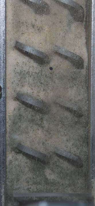
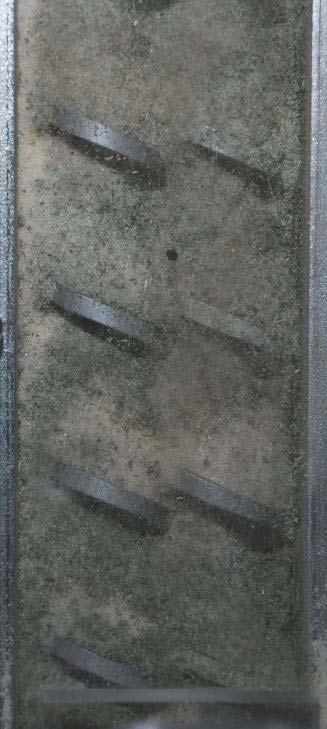
76 64 Figure 36. Cold flow mixing images of cornstover biomass and silica sand

77 65 Figure 37. Corn stover (1.0 mm), corn fiber (1.0 mm) and red oak biomass (0.75 mm) Different types and sizes of heat carrier materials were tested as well, as shown from left to right in Figure 38: sand, silicon carbide, alumina ceramic, 1.0 mm steel shot and 0.7 mm steel shot. A sample of operating conditions used during the shakedown trial phase is shown in Table 7. Figure 38. Sand, silicon carbide, alumina ceramic and steel shot heat carrier examples Table 7. Shakedown trials operating conditions T HC T R m b m HC d b d HC Q N2 ω A ( C) ( C) (kg/hr) (kg/hr) (μm) (μm) (SLPM) (RPM) Low High Calibration procedures are performed to determine the proper heater temperatures to maintain the desired heat carrier inlet temperature, T HC ( C). This corresponds to temperature T HC2 in Figure 31. The electrical guard heater around the reactor is set to a sufficient temperature, T R ( C), to minimize heat losses. This corresponds to temperature T RHc in Figure 33. The biomass mass feed rate, m b (kg/hr), is achieved by setting the auger speed rate on the biomass feeder, based on calibration procedures. Similarly, the heat carrier mass feed rate, (kg/hr), is achieved by setting the metering auger speed rate based on calibration procedures. The nominal biomass particle size, d b m HC

78 66 (mm), is achieved by the screen size used in a cutting mill or based on a standard sieving procedure. The nominal heat carrier particle size, d HC (mm), is as received by the manufacturer or based on a standard sieving procedure. The total volumetric flow rate of nitrogen into the system, Q N2 (SLPM), is controlled by a mass flow controller and is constant for the duration of a test. The rotational speed of the augers in the reactor, ω A (RPM), is achieved by setting the desired speed rate on the motor controller and is constant for the duration of the test. These operating conditions correspond to the simplified schematic of the reactor shown in Figure 39. m, T HC, d HC HC HEAT CARRIER PRODUCTS BIOMASS m b, d b A NITROGEN MOTOR HEATER TR REACTOR Q N2 SOLIDS Figure 39. Simplified reactor schematic with operational parameters shown In addition to testing various feedstocks and operating conditions, the shakedown trials were useful in refining the configuration and operation of the laboratory apparatus and finalizing the experimental procedures. Use of the different vapor outlet ports was investigated, as were different gas cyclones are condenser configurations. A final benefit of performing numerous shakedown trials was to demonstrate proof-of-concept of the reactor design, including steady-state operation. Several challenges and solutions were realized during the shakedown trial testing phase, and will not be discussed. Refer to Table 46 in Appendix A for details of the operating conditions performed for the shakedown trials, and Table 47 for the product distribution results. These tables illustrate that the procedures and the lab-scale system produce respectable mass balances and repeatable bio-oil yields within the range of reported literature for fast pyrolysis. This provided evidence and confidence to proceed with the experimentation phase of the research which will be described next.

79 67 CHAPTER 4. EXPERIMENTAL METHODS AND MATERIALS 4.1 Introduction For this research, a Response Surface Methodology (RSM) was selected to optimize the auger reactor design. This is a systematic methodology that allows for statistical investigation of responses that are a function of multiple factors (or variables), including any interaction effects between factors. For instance as discussed previously, the yields from biomass fast pyrolysis are known to be dependent on several conditions, thus these conditions need to be investigated simultaneously. As there is minimal data available on the auger reactor operating conditions, it is worthy to study the effects of these conditions on responses such as bio-oil yield and composition. RSM is a common experimental methodology used in the optimization of industrial processes [112, 113]. By constructing a theoretical model to estimate a given response, useful visual representations and equations can be developed to maximize or minimize the response. A thorough procedure was followed to determine a specific design of experiments to carry out the RSM, and will be discussed. 4.2 Experimental design The first step in a RSM is the selection of an appropriate experimental design. This selection is dependent not only on the number of factors of interest, but also the availability of resources. At least thirteen factors associated with the reactor system were identified that have possible effects on the product distribution and composition, as summarized in Table 8 along with the fast pyrolysis consideration affected by each factor. As the reactor system is a first generation design, factors that were assumed to have minimal effects were eliminated, as were factors that were not continuous ( categorical factors). As the lab-scale system was designed for a certain biomass feed rate (1 kg/hr), this was also eliminated as a factor. Furthermore, changing the biomass feed rate will alter the heat removal requirements for the bio-oil recovery system, potentially causing inconsistent system operation. In regards to the bio-oil recovery system, the design and operation of these components will affect the pyrolysis products; however these considerations are outside the scope of this research. Finally, the system was designed to provide heat for pyrolysis by means of the heat carrier material, so the reactor heater temperature was eliminated as a variable. According to the literature review performed on biomass fast pyrolysis and solids mixing, the remaining factors were all considered to be important enough to warrant further study. The heat

80 68 carrier feed rate, m HC, is easily adjustable by means of controlling the metering auger speed, and will intuitively effect the yields and composition because of the heat transfer effects. Similarly, the temperature of the heat carrier material, T HC, can be controlled by setting the electric heaters and the importance of reaction temperature is well documented. The rotational speed of the augers in the reactor, ω A, will affect the mixing behavior of the biomass and heat carrier, as discussed previously, which is assumed to then affect the heat transfer and devolatilization of the biomass. Finally, the flow rate of nitrogen, Q N2, effects the vapor residence time in the reactor and is easily controlled. Factor No. Table 8. Factor considerations for experimental design procedure Factor category Factor Fast pyrolysis consideration a Concern for selection 1 Type 5 Not continuous 2 Biomass Feed rate 1 Small turndown, system design properties 3 Particle size 1 Minimal effect compared to other factors 4 Moisture content 1 Minimal effect compared to other factors 5 Type 1,5 Minimal effect, not continuous 6 Heat carrier Feed rate 1,2 None 7 properties Particle size 1 Minimal effect, system capabilities 8 Temperature 1,2,~3 None 9 Auger rotational speed 1,2,~3 System capabilities 10 Reactor Vapor outlet port 3 Not continuous 11 configuration Total nitrogen flow rate 3 None 12 Reactor heater temperature 1,2 Control, system design 13 Product recovery Condenser temperature(s) 4 Outside scope of research Note: a - Fast pyrolysis considerations: (1) Rapid heat transfer, (2) Controlled reaction temperature, (3) Short vapor residence times, (4) Rapid cooling of reaction products, (5) Catalytic effects With four factors, n, selected (n = 4), the experimental design selection process was continued. As mentioned previously, a design was required to study possible interactions between factors and develop a response surface, so a 2 n factorial design was eliminated [113]. A 3 n factorial design could be used to develop this response surface; however 81 experiments are required for four factors which were deemed impractical to implement. Therefore, a Central Composite Design (CCD) was selected as a suitable design for the response surface methodology, and is often used in place of 3 n factorials to minimize experimental time and expenses [113]. Out of the possible CCD options, the commonly used circumscribed option was selected (can be referred to as CCC) as it allows for investigation of a large design space [112]. Other CCD options such as the inscribed (CCI), face centered (CCF), and Box-Behnken designs may require fewer runs than the CCC, but have a more restricted experimental space [112, 113]. The circumscribed central composite design is called such

81 69 because it has a 2 n factorial design imbedded within axial points as shown in Figure 40. Note this diagram only shows two factors, as all four factors can not be shown conveniently in two (or even three) dimensions. The axial points, also called star points [112], test conditions outside the main design space to help generate the curvature of the quadratic model. Note that typically all the points are given coded coordinates, with the so-called center-points having coordinates of (0, 0), and axial points at a distance α from the center point. Center point replicates are performed to help establish the experimental error [113]. 0, + -1,+1 FACTOR X2 COORDINATE +1,+1, 0 CENTER POINT 0, 0 FACTOR X 1 COORDINATE +, 0-1,-1 +1,-1 0, - Figure 40. Central Composite Design schematic for two factors Image adapted from Kuehl [113] The number of experiments, N, and the α value required for a CCD with n factors and m center point replicates are calculated by Equations 3 and 4 respectively. n N = n + m Equation 3 α = (2 n ) 1/4 Equation 4

82 70 For 6 center point tests (m = 6), this results in a four factor, five level central composite design requiring 30 experiments and an α value of 2.0. This α value implies that, for a given level, the step from the factorial point (1) to the axial point (α) is the same as from the center point (0) to the factorial point (1). The levels for the design were chosen based on information gathered or determined during the literature review, engineering design and shakedown trial portions of the project. In selecting levels for this type of design, there is a tradeoff between what the experimental apparatus can physically achieve and what will allow for a suitable response surface to be developed. The final factors and levels chosen for the design are shown in Table 9, with notation as discussed previously. ` Table 9. Selected factors and levels for experimental design Level T HC ( C) Factor Q N2 (SLPM) ω A (RPM) m HC (kg/hr) α α As noted, the resulting model from this experimental design procedure is quadratic (second order) with 15 coefficients as shown in Equation 5, and serves to estimate the response surface [113]. There is an intercept term, β o, and 14 remaining coefficients associated with each factor (4), each of the interaction terms between factors (6), and each factor squared (4). Note that the response in Equation 5, Y i, is general and different models can be developed for any number of responses. Y = β i + β + β + β o T T T + β HC HC 2 HC 1 T Q m + β N2 HC 22 HC + β + β + β Q N2 Q T HC ω + β N2 N β ω ω A m 2 A 3 + β HC ω + β A 23 + β 44 + β Q 34 m 4 N2 ω A 2 HC m ω HC A m HC Equation 5 As an expansion of Table 9, a list of all the experiments performed is shown in Table 10 in the coded format. Note the three sections shown: 16 factorial design experiments, 8 axial point experiments, and 6 center point experiments with the same conditions.

83 71 Table 10. Final central composite design, coded experiments 2 n factorial treatment design (n = 4) 2n axial points (n = 4) Center points (m = 6) T HC ( C) Factor Q N2 (SLPM) ω A DOE # (RPM) m HC (kg/hr) α α α α α α α α Similarly, Table 11 is shown for the actual experimental conditions. Note the second column shows the order the experiments were performed in. Due to lengthy and complex calibration procedures for the heat carrier mass feed rate, m HC, and inlet temperature, T HC, the experiments were randomized within blocks of heat carrier feed rates that were grouped together. While it is often preferred to completely randomize the experiments including the center point tests, minimization of experimental error is also an important consideration. Calibrating the system for one group of feed rates and completing that block of experiments was determined to be the best option for maintaining and repeating the operating conditions of the system.

84 72 Table 11. Final central composite design, actual experiments 2 n factorial treatment design (n = 4) 2n axial points (n = 4) Center points (m = 6) T HC Factor DOE Run V N2 ω A m HC # # ( C) (SLPM) (RPM) (kg/hr) Experimental materials The biomass used for this research was northern red oak (Quercus Rubra L.) obtained from Wood Residuals Solutions (Montello, WI). Red oak is a hardwood species in the Beech family used for lumber, and is native to most of the eastern United States [114]. This biomass was chosen based on two factors: superior performance as determined during shakedown testing, and the ability to compare the results to other pyrolysis studies using oak wood. Often used as animal bedding, this oak wood was kiln dried before delivery in a super-sack to the BECON facility in Nevada, IA. Here it was first processed into more homogenous sized particles in an Art s Way Manufacturing stationary

85 73 hammer-mill with a 1/8 screen size, as shown in Figure 125 of Appendix C. Further size reduction was accomplished using a Retsch SM 200 heavy duty cutting mill with a 0.75 mm screen size, as shown in Figure 126 of Appendix C. This size was selected to minimize heat transfer limitations. Other than size reduction, no further drying or pre-treatment steps were carried out before testing. After grinding, the biomass was stored at ambient conditions in 5 gallon plastic buckets with sealed lids. The red oak biomass is shown in Figure 41 from left to right: as received, after hammer mill processing with a 1/8 screen, and after knife mill processing with a 0.75 mm screen. Figure 41. Red oak biomass samples of three different grind sizes Soil Control Lab (Watsonville, CA) analyzed the composition of the red oak biomass on April 21, 2009 with results as shown in Table 12. These results shown that cellulose, hemicellulose and lignin account for over 93% of the mass, and that the biomass has a low ash content. Table 12. Red oak biomass composition 1 Component Results Notes on method Fats, Waxes and Oils 0.1 Ether extract Resins 1.5 Alcohol extraction Water soluble polysacchardies 1.7 Hot water extraction Hemicellulose 20.0 Hydrolysis with 2% HCl Cellulose 29.8 Hydrolysis with 80% H 2 SO 4 Protein 0.5 Total Nitrogen X 6.25 Lignin-humus 43.3 Total carbon X Ash deg. C Total 97.3 Other or missing components 2.7 Percent Moisture Percent dry weight, unless otherwise noted

86 74 The elemental composition of the biomass was determined with a LECO TruSpec CHNOS analyzer as shown in Figure 127 of Appendix C. Carbon, hydrogen and nitrogen were analyzed based on the ASTM D5373 standard, and ASTM D4239 was referenced for the sulfur analysis. Thermal gravimetric analysis methods and ASTM D5142 were used to determine the ash content and perform the proximate analysis of the biomass using a Mettler Toledo Star e System as shown in Figure 128 of Appendix C. The higher heating value of the biomass was determined using standard calorimetric methods with a Parr 1341EB oxygen bomb calorimeter as shown in Figure 129 of Appendix C. These analyses, performed in triplicate, are summarized in Table 13. Table 13. Red oak biomass ultimate and proximate analyses Ultimate Analysis (%-wt., ar) Carbon Nitrogen Hydrogen Sulfur Ash Oxygen a Average Standard deviation Proximate Analysis (%-wt., ar) HHV b Moisture Volatiles Fixed carbon Ash Total (MJ/kg) Average Standard deviation Notes: a - Oxygen by difference. b - Higher heating value. ar - As received The heat carrier used for this research was AMASTEEL cast steel shot from Irvin Industries (Ann Arbor, MI), and is typically used for abrasive or shot peening applications [115]. Steel shot was selected as a heat carrier based on superior performance as determined during shakedown testing. Compared to sand, steel shot is denser and more thermally conductive, and is less likely to clog upon becoming moist. Though not important for this study, a potential downside to steel shot compared to sand is its inability to be conveyed pneumatically. The steel shot size used was S-280, and though the 280 indicates a nominal diameter of in (0.71 mm), the official designation is a distribution based on SAE J827 standards as shown in Figure 42. The composition of the steel shot and select properties (as provided by Irivin Industries and not tested) is shown in Table 14 [115].

87 75 To ensure similar composition of steel shot between tests, 1500 lbs (680.4 kg) was obtained from a single manufactured lot through LS Industries (Wichita, KS). The steel shot was stored at ambient conditions in sealed 50 pound bags, and fresh steel shot was used for each experiment. Figure 42. SAE J827 steel shot size distribution Image source: Marco U.S.A. [116] Table 14. Steel shot composition and select properties Element %-wt. Iron > 96.0 Carbon < 1.20 Manganese < 1.30 Silicon < 1.20 Chromium < 0.25 Copper < 0.20 Nickel < 0.20 Specific gravity (@ 15.6 C) > 7.6 Meltin g point ( C) Testing procedures The RSM was carried out by performing three major types of testing: reactor operation to determine the fast pyrolysis product distribution, analytical testing to determine the composition of the bio-oil and biochar that was produced, and statistical methods to analyze and evaluate the data.

88 76 Extensive graphical methods were also carried out to interpret and analyze the results. These three procedures will be discussed independently next Product distribution The product distribution for each of the CCD runs was determined by performing experiments with the lab-scale reactor system previously described. The product yields are determined gravimetrically in the case of bio-oil and biochar while the mass of non-condensable gas is calculated from its volumetric yield. With notation as discussed previously, the operating conditions for the experiments are shown Table 15. Table 15. Experimental operating conditions T HC T R m b m HC d b d HC Q N2 ω A ( C) ( C) (kg/hr) (kg/hr) (μm) (μm) (SLPM) (RPM) The biomass feed rate is controlled by setting the motor speed on the biomass feeder, and is calibrated to feed a relatively constant mass rate. As the feeder conveys material volumetrically, small fluctuations in bulk density will vary the mass feed rate slightly. Therefore, the rate is given as an average over the duration of an experiment. Calibration tests are a minimum of ten minutes each and performed for at least five speed settings. Before each pyrolysis run, the moisture content of the biomass is determined by heating a 4 g sample to 105 C using an Omnimark Mark 2 Standard moisture scale as shown in Figure 130 of Appendix C. Approximately 1200 g of prepared biomass is then weighed with a 2100 x 0.01g Ohaus Explorer scale and placed into the feed hopper. This mass is denoted as m b in the mass balance schematic shown in Figure 43, and recorded on the mass balance worksheet as shown in Figure 44. Note the biomass feed is not begun until the system has reached operating temperatures. Similarly, the steel shot feed rate is controlled by setting the motor speed on the heat carrier metering auger motor controller. The calibration procedure includes recording the time required to feed a known amount of heat carrier through the reactor, and is performed for a minimum of one hour of feed time for three different speed settings. Typical rotating speeds for the heat carrier metering auger are RPM. Depending on the feed rate required for a specific experiment, approximately 23 kg of steel shot is then weighed and placed in the feed system. A 64 kg x 0.1g Sartorius FBG-64

89 77 EDE-H scale is used to determine the mass of the heat carrier. The steel shot mass is denoted as m HC in Figure 43, and is recorded on the mass balance worksheet shown in Figure 44. The important mass balance symbols used in Figure 44 are listed in Table 16. Figure 43. Reactor system schematic showing mass balance Refer to Table 16 for nomenclature Important components are then cleaned, weighed and installed on the system. These include the solids canister, the cyclone catch, condenser 1 (SF1) and condenser 2 (SF2), the ESP collection bottle (SF3), and the third condenser coil (SF4). The masses are all recorded on the mass balance worksheet. Each of these components is weighed on the Ohaus scale, except the condensers which are each weighed on the Sartorius scale separately. The electric heaters associated with the heat carrier system and reactor, including heat tapes, are then initiated to began the warm-up phase of the procedure. The down-stream heat tapes inbetween the reactor and the condensers are set to 485 C. The reactor heater set point is constant for

90 78 all the tests, and the set point temperatures for the remaining heaters are determined based on suitable calibration procedures. These procedures are performed to determine the correct heater temperatures to maintain a steady heat carrier inlet temperature, T HC, as a function of the heat carrier feed rate and the final desired temperature. The set points for the heat carrier heaters range from approximately 40 C C above the required heat carrier inlet temperature, with 60 C - 70 C being the most common range. The warm-up phase takes approximately two hours. Table 16. Description of symbols used in mass balance procedure Symbol m NCG m HC m b m S m cy m C m SF1 m SF2 m SF3 m SF4 m bio-oil m b,h2o Description Mass of non-condensable gas Mass of heat carrier Mass of wet biomass Mass of solids (heat carrier and biochar) Mass of biochar collected in cyclone Total mass of biochar Mass of stage fraction 1 bio-oil Mass of stage fraction 2 bio-oil Mass of stage fraction 3 bio-oil Mass of stage fraction 4 bio-oil Mass of total bio-oil Mass of moisure in wet biomass Early in the warm-up phase, cooling water flow is initiated to the biomass injection auger at 12 GPH (0.757 L/min), and condensers 1 and 2 at 20 GPH (1.26 L/min) each. The chiller is started to provide cold water to condenser 2. Around 5 gallons of Ice is added to the container where the third condenser is located. The nitrogen flow is also initiated during the warm up phase, and the total volumetric flow rate is controlled with a mass flow controller based on the desired CCD value. As described previously, four gas rotometers are used to split the total flow between various other components on the system. As shown in Table 17, the volume fraction of flow through each rotometer remains constant for each flow rate. Before the pyrolysis phase of an experiment the nitrogen gas is vented. After sufficient heat carrier temperatures are attained, the augers in the reactor are initiated and set to the desired CCD value using the motor controller. The controller is set to a percentage of 180 RPM (the maximum speed). For instance the center point setting is 30%, corresponding to 54

91 79 RPM. The heat carrier feed rate is begun and a lab timer is started. The LabVIEW program is then started to observe system temperatures and pressures during the heat carrier feeding phase. The time required for the heat carrier feeding phase is dependent on the feed rate, and ranges from approximately 25 minutes to over one hour to reach steady state conditions. Once steady heat carrier inlet temperatures have been attained, the pyrolysis phase can be initiated. Table 17. Gas rotometer settings for experiments Total flow rate Q N2 (sl/min) Purge flow rate through rotometers (sml/min) Reactor (end) Heat carrier system Reactor (main) Biomass feed system %-vol. of total The fast pyrolysis phase of the experiment is begun by switching the flow of purge nitrogen from the vent to the Micro-GC and gas volume meter. The ESP is then energized to -15 kv and the LabVIEW program is set to begin collecting temperature and pressure data. The Micro-GC program and the biomass feed are now initiated, while a lab timer is started and the volume reading on the gas meter is recorded. Gage pressure readings at the volume meter are observed and recorded periodically on the mass balance worksheet as shown in the lower right portion of Figure 44. The pyrolysis phase is continued until the biomass or heat carrier material is depleted, or until the bio-oil collection bottles become full, and typically lasts around one hour. The shutdown procedure begins with stopping the biomass feed and the lab timer, and recording the final volume reading on the gas meter. This is followed by stopping the heat carrier feed and lab timer. The heaters are then shutdown, and the water and nitrogen flows continue to cool the system while the temperatures are observed. After the water and nitrogen are shut down, the condensers, the ESP bottle and third condenser coil are removed. The final masses are determined and recorded on the mass balance worksheet. After cooling to room temperature, the char catch and the solids canister are removed and the masses are determined and recorded. Any biomass and heat carrier material remaining in the system is also removed and the masses are determined and recorded.

92 80 Run date Reactor heater set point temperature ( C) 550 Run ID Run No./ DOE No. Heat carrier inlet temperature ( C) Heat carrier heater set point temperature ( C) Run Jared Brown N 2 volutermic flow rate (SLPM) operators Auger rotational speed (% of 180 RPM) Vapor port 1 Heat carrier feed rate (kg/hr) Biomass Heat Carrier NCG Note Value 1 Value 2 Unit Note Value 1 Value 2 Units Note Value Units Moisture Canister Initial - %-wt. - g content mass volume m 3 Initial mass Initial mass Final volume m 3 Bucket 1 g Bucket 1 g Note Values Bucket 2 g Bucket 2 g Bucket 3 g Bucket 3 g Final mass Final mass Hopper 1 g Canister - g Hopper 2 g In reactor g Below auger g Bucket 1 g Feed tube 1 g Bucket 2 g Feed tube 2 g Bucket 3 g Vaccum g Bucket 4 g Misc. g Bucket 5 g Feed rate Feed rate Start/stop Time Start/stop Time Elapsed time - min Elapsed time - min Bio-oil Biochar (cyclone) Note Initial Final Units Note Initial Final Units Condenser 1 g Catch g Condenser 2 g In cyclone g ESP (SF3) g Misc. 1 g Tube (SF2-3) g Coil (SF4) g NOTES Condensers g SF1 bottle g SF2 bottle g SF3 bottle g Misc. 1 g Misc. 2 g Rotometer settings ume meter NCG: Pressure readings (in-h 2 O) at vol Figure 44. Mass balance worksheet for experiments This procedure is repeated for all the central composite design experiments. Based on the data collected during the mass balance procedures, the product distribution can be completed as follows. As shown in Equation 6, the bio-oil yield on a wet basis (wb) is given as a weight percentage of the original wet biomass mass, m b. The total collected bio-oil mass, m bio-oil, is a sum of the individually collected fractions, SF1-SF4, as shown in Figure 43. Y m + m + m + m m bio oil Equation 6 m SF1 SF2 SF3 SF4 bio oil,wet (% wt., wb) = = m b b

93 81 However the weight of moisture carried in by the biomass, m b,h2o, varies slightly between experiments, so it is often appropriate to normalize the bio-oil yields to a dry basis (db). This is done by calculating the yield on a dry biomass basis, and with the biomass moisture content removed from the bio-oil mass, as shown in Equation 7. Note that the biomass moisture content is determined with the moisture scale as discussed previously. Also note that this calculation does not remove any reaction water contained in the bio-oil, only the original biomass moisture mass. Y m m bio oil b,h2o bio oil, dry (% wt.,db) = Equation 7 m b m b,h2o The calculation of the biochar yield on a wet biomass basis is shown in Equation 8, with notation as discussed previously and shown in Figure 44. ( m m ) S HC + mcy mc Y C (% wt., wb) = = Equation 8 m m b b For notation used in Equations 6 8, refer to Table 16. As noted previously, the noncondensable gas stream is analyzed with a Varian CP-4900 Micro-GC, connected to Galaxie Chromatogrpahy 1.9 software on a Dell D630 laptop. A Varian Molsieve 5A column is used for detecting hydrogen, oxygen, nitrogen, methane and carbon monoxide (110 C injector temperature, 100 C oven temperature, with argon carrier gas at kpa). A Varian Pora Plot Q column is used to detect carbon dioxide, ethylene, acetylene and ethane (110 C injector temperature, 58 C oven temperature, with helium carrier gas at kpa). Each gas sampling program lasts between 3 and 4 minutes, and approximately 15 analysis points are collected during the steady state portion of an experiment. The Micro-GC is shown in Figure 131 of Appendix C. The non-condensable gas yield is determined by applying the ideal gas law, in conjunction with gas analysis data from the Micro-GC and gas property data collected at the gas meter (temperature, pressure and volume) as shown in Figure 132 of Appendix C. A characteristic sample output from the Micro-GC (Run #24/DOE #2) is shown in Figure 45, noting the steady state region where the pyrolysis reactions are occurring.

94 82 tration (%-vol.) Gas concen Steady state region Analysis number Note: Run #24/DOE #2. Heat carrier temperature = 575 C, Heat carrier feed rate = 12 kg/hr, N 2 flow rate = 3.5 sl/min, Auger speed = 58.5 RPM. N2 H2 CO CH4 C2H6 C2H4 CO2 Figure 45. Micro-GC gas analysis profile for Run #24 The numerical results that correspond to this graphical representation are shown in the third column of Table 18, noting the Micro-GC analyzer was able to detect approximately 96.4%-vol. of the gas. Therefore, the concentration of gas species needs to be normalized to account for the unknown portion by assuming the known composition of gas sums to 100% of the volume. Then, based on molecular weights of each gas species and the normalized concentration, the weighted molecular weight can be determined for each species contribution. The sum of these, shown in the last column of Table 18, is assumed to be the apparent molecular weight of the non-condensable gas mixture, M NCG (kg/kmol). During the steady-state operation as shown in Figure 45, the volume of nitrogen passing though the meter is also known based on the Micro-GC gas composition results. This allows for calculation of the total volume of non-condensable gas produced, and the total gage pressure and gas temperature at the meter inlet are known, so the mass (and then the yield) of the NCG can be estimated by applying the ideal gas law. As shown in Table 18, 34 kg/kmol is a common value for the apparent molecular weight of the non-condensable gas mixture.

95 83 Compound, i Table 18. Non-condensable gas analysis for Run #24 Formula Known concentration (%-vol) M i (kg/kmol) Normalized concentration (%-vol) y i Nitrogen free (kmol/kmol) y i M i Nitrogen free (kg/kmol) Nitrogen N Hydrogen H Carbon monoxide CO Methane CH Ethane C 2 H Etheylene C 2 H Carbon dioxide CO Unknown Sum Note: Data from Run #24/DOE #2. Heat carrier inlet temperature = 625 C, Heat carrier feed rate = 12 kg/hr, N 2 flow rate = 3.5 sl/min, Auger speed = 58.5 RPM A typical temperature profile of an experiment is shown in Figure 46, with data presented from Run #20/DOE #24. The heat carrier inlet temperature, T HC, is shown to increase during the warm-up phase, and then level out to the desired value (625 C for this particular experiment). The gas phase temperatures inside the reactor are seen to increase with time as the heat carrier is fed, and then decrease once the biomass feeding begins. This happens because the cold biomass enters and absorbs heat from the reactor. However the reactor temperatures quickly steady out to a temperature ranging from approximately C, depending on the axial location in the reactor. The condenser inlet temperature is maintained above approximately 430 C to prevent preliminary condensation of pyrolysis products, and is seen to quickly increase once biomass feeding begins and hot vapors leave the reactor. The downstream temperatures associated with the bio-oil recovery system are shown in Figure 47, and the ranges are based on the temperature of the vapor products entering the reactor, which is a function of the heat carrier temperature, T HC. The wall temperature of the first condenser quickly increases once biomass is fed into the reactor and hot vapors evolve. Note the noncondensable gas leaving the final condenser is typically less than 15 C, however it increases to above ambient (approximately 30 C) by the time it reaches the volume gas meter after passing through the vacuum pump and Micro-GC.

96 84 Temperature ( C) Start heat carrier feed HC (Inlet) Reactor 1 Reactor 2 Reactor 3 Reactor 4 SF1 (Inlet) SF1 (Wall) SF3 (Inlet) Start biomass feed Time (hours) Approximate steady state region Note: For Run #20/DOE #24. Heat carrier inlet temperature = 625 C, Heat carrier feed rate = 15 kg/hr, N 2 flow rate = 2.5 sl/min, Auger speed = 54 RPM Figure 46. Temperature profile example for Run #20 Figure 47. Typical bio-oil recovery system temperatures

97 Product analysis After a given pyrolysis experiment was complete, the bio-oil and biochar collected were subjected to a number of analytical tests to characterize the physical properties and chemical composition. As applicable, the analysis methods closely follow the recommendations for testing as commonly reported in related literature - refer to Oasmaa et al. for one such study [117]. Note that the methods will only be described briefly here, and complete laboratory standard operating procedures (SOPs) were referenced during the analysis. Also, not all analyses were performed for all the bio-oil fractions or all of the biochar samples. Sample preparation. After cooling, biochar samples from the cyclone were stored in sealed, labeled plastic bags. Bio-oil fractions were immediately stored in sealed, separate and labeled plastic bottles (250 ml HDPE bottles for SF1 SF3, and 50 ml polypropylene bottles for SF4) in dark, refrigerated conditions around 5 C. Prior to any testing procedures, all bio-oil samples were removed from the refrigerator, and homogenized by vigorously shaking the sample bottle by hand for a minimum of one minute, followed by stirring at 1700 RPM (Eastern Mixers 5VB-C) for a minimum of one additional minute. Some tests require additional homogenization techniques and will be discussed. Various lab balances are used as part of the analytical test procedures, with the numbers in parenthesis corresponding to the test method(s) that are described below. a. Cole-Parmer Symmetry PA220, 220 g x 0.1 mg (1, 4, 8) b. Sartorius ME 254S, 250 g x 0.1 mg (2, 3) c. Mettler Toledo MX5, 5 g x 1 μg (5, 7) d. Mettler AE 100, 110 g x 0.1 mg (6) 1. Moisture content. Moisture content is an important fuel property because it affects combustion behavior; however it is also used as an indication of bio-oil quality and has implications for stability. After the bio-oil preparation techniques were performed, moisture content of bio-oil was determined by the common Karl-Fischer (KF) titration method. This was accomplished by using a MK5 KF Moisture Titrator as shown in Figure 133 of Appendix C, and referencing ASTM E203. This is an accepted method for determining the moisture content for pyrolysis liquids. A μg sample is injected into the instrument, and is dissolved in a solvent (Hydranal Working Medium K) and a reagent (Hydranal Composite 5K) that reacts with and consumes the water present. A syringe is weighed before and after sample injection to determine the sample mass.

98 86 Calibration standards are performed with D.I. water prior to testing. Moisture content is reported on a percent weight of the wet bio-oil, denoted by (%-wt., wb). 2. Water insoluble content. Bio-oil can generally be separated into water soluble and water insoluble fractions, though some components are partially soluble which leads to inconsistencies in definitions used in related literature. Nonetheless, the water insoluble fraction is often referred to as the pyrolytic lignin portion of the bio-oil, and is an important property for bio-oil upgrading considerations and may reveal insight on the pyrolysis reactions. The method starts by placing 20 ml of sample in a bottle and homogenizing in an ultrasonic water bath (Branson B-52) for 30 minutes, followed by additional homogenization on a laboratory shaker table (Thermo-Scientific Max Q 2500) for 30 more minutes. From this bottle, 2 g bio-oil samples are retrieved and 10 g of D.I. water is added to each. The mixtures are homogenized using a vortex mixer for 1 minute, after which 10 additional grams of water is added. This procedure is repeated twice more so the final mass ratio of water to bio-oil is 20:1. The final mixture is sonicated for an additional 30 minutes, placed on the shaker table for one hour, and rotated in a centrifuge (Fischer Scientific accuspin 1) at 2500 RPM for 20 minutes to fully solubulize any miscible components. Filter paper (Whatman No. 42) is weighed after drying at 105 C for 15 minutes and cooled in a desiccant vessel for 15 minutes. The prepared sample is poured over this filter paper, assisted by a vacuum pump (Fischer Scientific MaximaDry), where the water soluble components pass through the filter and the water insoluble components are left on the filter. The filter paper, sample bottle and lid are dried at 50 C for 20 hours and cooled in a desicca nt vessel for 15 minutes. The masses of the filter paper, sample bottle and the sample lid are then determined and recorded. The water insoluble content is then determined by subtracting the final weight of the filter, sample bottle and lid from the initial weights, divided by the mass of the total bio-oil sample. Insoluble content is reported on a percent weight of the wet bio-oil, denoted by (%-wt., wb). 3. Solids content. The solids content of the bio-oil is an important fuel property because it affects combustion behavior and particulate emissions. As noted, the solids suspended in bio-oil are typically fine biochar particles that were not removed by the gas cyclone, but could include sand particles in the case of fluidized beds. To determine the solids content, a procedure similar to that for determining water insoluble content is used, except methanol is used as a solvent rather than water. This allows for all compounds to be solubulized, except particulate matter. A 1 g sample of bio-oil is added to 12 g of ACS grade methanol, and homogenized using a vortex mixer. Filter paper (Whatman No. 42) is weighed after

99 87 drying at 105 C for 15 minutes and cooled in a desiccant vessel for 15 minutes. The prepared sample is poured over this filter paper, assisted by a vacuum pump, where the methanol soluble components pass through and the methanol insoluble components are left on the filter. The filter paper is dried under a fume hood for 15 minutes, dried at 105 C for 30 minutes, and cooled in a desiccant vessel for 15 minutes. The final mass of the filter paper is determined, and the change in mass divided by the bio-oil sample mass is the solids content, reported on a percent weight of the wet bio-oil (%-wt., wb). 4. Higher heating value. The higher heating value, or heat of combustion, of bio-oil is a major fuel property of interest. Using a calorimeter, the chemical energy stored in a fuel sample (solid or liquid) is released during combustion, and is quantified by measuring the temperature change of 2000 g of water surrounding the combustion vessel. As the instrument is well-insulated (assumed to be adiabatic), the energy released from the combustion reaction is completely absorbed by the water, reflected as in increase in temperature that is precisely measured. A Parr 1341EB oxygen bomb calorimeter was used as shown in Figure 129 of Appendix C. The instrument includes a stainless steel vessel that is pressurized to 30 atmospheres with oxygen to ensure complete combustion. The procedure for determining the heating value is modified from ASTM D240 for liquid hydrocarbon fuels. The bio-oil sample mass is typically 0.7 g, and approximately 0.2 g of mineral oil is often added to the sample to aid in complete combustion. This is especially required for high water content samples, and is accounted for in the combustion value calculations. The higher heating value is typically reported in units of (MJ/kg) on a wet bio-oil basis. 5. Thermal gravimetric analysis. Thermal gravimetric analysis, or TGA, is used to determine the mass change of a sample with increasing temperature and time. This data is used for the proximate analysis, which gives the percent weight of moisture, volatiles, fixed carbon and ash. As noted previously, a TGA/DSC Mettler Toledo Star e System is used (see Figure 128 in Appendix C), and ASTM D5142 is referenced for analyzing biochar. Calcium carbonate is used as a reference standard. Sample masses for bio-oil range from mg, with 80 mg being a common value, and biochar sample masses range from mg, with 15 mg being a common value. The program method for the TGA is as shown in Table 19. Note that the moisture value as determined by TGA is much higher than as determined by KF titration methods, because bio-oil contains many compounds other than water that volatilize at temperatures less than 105 C. As such, for this study, the main property of interest as determined by TGA is the ash content of the bio-oil and biochar.

100 88 Table 19. Thermal gravimetric analysis program method Hold time Temperature ( C) Step (min) Start Stop Heating rate ( C/min) Purge gas Flow rate (ml/min) Ramp N Hold N Ramp N Hold N Hold Air Elemental composition. The elemental composition of interest for bio-oil and biochar includes the percent weight amount of carbon (C), hydrogen (H), nitrogen (N), oxygen (O) and sulfur (S) present. In combination with the ash content, this represents the ultimate analysis of the product. As discussed previously, the elemental composition is determined with LECO TruSpec CHN/O/S analyzers (see Figure 127 in Appendix C). This system completely combusts fuel samples (solid or liquid), and analyzes the evolved gas products to determine the composition. Typical sample weights are 0.1g and 0.2g for the C/H/N analyses and the S analysis, respectively, for both bio-oil and biochar. ASTM D5291 and ASTM D1552 are referenced for analyzing the C/H/N and S content in the bio-oil, respectively, and ASTM D5373 and ASTM D4239 are referenced for analyzing the C/H/N and S in the biochar, respectively. With C, H, N, S and ash known, the oxygen content is determined by difference for this study. 7. Total acid number. The total acid number, or TAN, is a valuable property of interest when comparing bio-oil to petroleum based fuels. In general, this test determines the amount of potassium hydroxide (KOH) required to neutralize a 1 gram quantity of sample, given in units of milligrams KOH per gram of sample (mg/g). A Metrohm 798 MPT Titrino titrator is used for the TAN analyses, as shown in Figure 134 of Appendix C, and ASTM D664 is referenced for the procedure. A solvent of 50%-wt. toluene, 49.5%-wt. 2-propanol and 0.5%-wt. D.I. water is prepared at a volume of 100 ml and analyzed as a blank to calibrate the instrument, after which 5.0 g of TAN standard (Fischer Scientific ST , 2.5 mg KOH /g) is added to the solvent and analyzed to verify the instrument operation. Then a 0.2 g sample of bio-oil is dissolved in 5 ml dimethylformamide (DMF), and added to 75 ml of methanol before analysis. 8. Gas chromatography/mass spectrometry (GC/MS). GC/MS methods are used to help characterize the chemical composition of bio-oil. A Varian CP-3800 GC and Saturn 220 GC/MS are used as shown in Figure 135. The capillary column is a CP-19CB/CP 8722 (86% dimethylpolysiloxane phase, 14% cyanopropyl-phenyl), with dimensions of 60 m x 0.25 mm x 0.25

101 89 μm (length x ID x film thickness). The GC portion of the instrument vaporizes the injected sample (99.999% helium is used as a carrier gas at 1 ml/min) and separates compounds based on the column selection described. The compounds are then analyzed and detected in the MS portion of the instrument using the electron ionization mode. Ideally, specific compounds are detected which produce specific signals at a corresponding retention times. A m/z range from 30 to 300 is scanned, and standard mass spectra with 70 ev ionization energy is recorded. The Varian GC/MS software package includes a NIST library that is used to match the resulting mass spectra for peak identification if necessary. The injector temperature on the instrument is maintained at 250 C, and the GC/MS interface is maintained at 235 C. The initial oven heating begins at 45 C for four minutes and is brought to the GC/MS interface temperature at a heating rate of 3 C/min (63.3 minutes). The GC/MS interface temperature is then maintained for an additional 13 minutes. Bio-oil samples on the order of 0.25 g are diluted in HPLC grade methanol at 4.5%-wt (95.5%-wt. methanol). The methanol solution is prepared with phenanthrene as an internal GC/MS standard at a concentration of 0.02%-wt. The bio-oil is homogenized with the methanol by mixing with a vortex mixer, and then filtered with a 0.2 μm filter before placing into a GC/MS sample vial. In addition to the phenatnthrene standard, the GC/MS instrument is calibrated to quantify the concentration of 32 additional compounds as shown in Table 20. In addition to acetic acid and levoglucosan (two common bio-oil constituents), the 30 remaining compounds are grouped into the broad chemical families of furans, phenols, guiacols, syringols, and other GC/MS as shown. 9. Viscosity. Viscosity of bio-oil is an important property because it affects the fluid flow characteristics in pipes, pumps and injection nozzles on utilization equipment. Dynamic (absolute) viscosity measurements are made with a Brookfield LV-DV-II+ Pro viscometer as shown in Figure 136 of Appendix C. This instrument determines the viscosity of a fluid by sensing the torque required to rotate a shaft spinning at a constant rotational speed within the fluid. Depending on the composition of a given bio-oil sample, different shaft attachments (spindles) are used to attain a minimum amount of torque required by the instrument. Depending on the spindle used, 3 16 ml of sample is required for analysis. In general, more viscous samples require a smaller diameter spindle. The spindle speed is adjusted to maintain an adequate torque reading (in-between 10% and 90% of the maximum), and a Thermo-Haake B7 water heater is used to maintain the temperature of a water jacket around the sample vessel. For this study, viscosity measurements were made at 40 C, which is a commonly reported value.

102 90 There are many other bio-oil and biochar analysis methods available for determination of other properties; however these are some of the most commonly reported methods and will indicate a broad overview of the product composition. Table 20. Chemical compounds quantified by GC/MS analysis Chemical compound Chemical formula Acetic (ethanoic) acid C 2 H 4 O 2 1,6-Anhydro-β-D-glucopyranose (Levoglucosan) C 6 H 10 O 5 Furans 2-furancarboxaldehyde (Furfural) C 5 H 4 O 2 2-Furanmethanol (Furfuryl alcohol) C 5 H 6 O 2 3-Methyl-2(5H)-furanone C 5 H 6 O 2 2-Furancarboxaldehyde, 5-methyl- C 6 H 6 O 2 Phenols Phenol C 6 H 6 O Benzene-1,4-diol (Hydroquinone) C 6 H 6 O 2 Phenol, 2-methyl- (o-cresol) C 7 H 8 O Phenol, 3-methyl- (m-cresol) C 7 H 8 O Phenol, 4-methyl- (p-cresol) C 7 H 8 O Phenol, 2,4-dimethyl- C 8 H 10 O Phenol, 2,5-dimethyl- C 8 H 10 O Phenol, 2-ethyl- C 8 H 10 O Phenol, 3-ethyl- C 8 H 10 O Phenol, 3,4-dimethyl- C 8 H 10 O Guaiacols Phenol, 2-methoxy- C7H8O2 Phenol, 2-methoxy-4-methyl- C 8 H 10 O 2 4-OH-3-methoxybenzaldehyde (Vanillin) C 8 H 8 O 3 Phenol, 4-ethyl-2-methoxy- C 9 H 12 O 2 2-Methoxy-4-(2-propenyl)phenol (Eugenol) C 10 H 12 O 2 Phenol, 2-methoxy-4-(1-propenyl)-, (E)- C 10 H 12 O 2 Syringols Phenol, 2,6-dimethoxy- C9H12O3 4 methyl 2,6 dimethoxy phenol C 9 H 12 O 3 Ethanone, 1-(4-hydroxy-3,5-dimethoxyphenyl) C 14 H 12 O 2 Other GC/MS compounds 1-Hydroxy-2-Propanone C 3 H 6 O 2 propane-1,2,3-triol (Glycerin) C 3 H 8 O 3-Hydroxy-2-butanone C 4 H 8 O 2 2-Furancarboxaldehyde, 5-(hydroxymethyl) C 6 H 6 O 3 2-methyl-2-cyclopenten-1-one C 6 H 8 O 1,2-Cyclopentanedione, 3-methyl- C 6 H 8 O 2 2H-Pyran-2-one C 6 H 10 O 3

103 Data analysis and hypothesis testing As the product distribution tests were completed, the yields of bio-oil and biochar were calculated, as were the resulting mass feed rates of biomass and heat carrier. The Micro-GC data was analyzed, and the average temperature at the gas meter was determined from the LabVIEW data to help calculate the NCG yield. The analysis of the NCG was extended to convert the composition on a volume basis to a mass basis composition. With the mass of NCG calculated as discussed previsouly, as well as an apparent molecular weight based on the normalized and weighted gas composition, the number of moles of NCG produced can be calculated. Then, based on the molar concentration as determined by the Micro-GC and each gas species molecular weight, the mass of each species could be determined. Finally, temperature data was also analyzed to determine the average heat carrier inlet temperature over the duration of the biomass feed time. The SAS-JMP 6.0 statistical software package was utilized to perform the regression modeling procedures. The parameters of the experimental design (type, factors, levels, and number of center points) were input into the program, along with the raw data values for a given response. The standard least squares method was selected to run the model, first with all coefficients present ( full model ) as show previously in Equation 5. The resulting model data was then analyzed graphically and statistically. The residuals (distance of actual experimental data from the predicted values) were first observed to ensure the experimental measurements were not related to each other in some way, which would decrease the validity of the model. The assumptions required to perform a linear regression model will not be discussed, but were reviewed by Kuhel [113] and Levine et al. [118]. The assumptions required to perform a linear regression are assumed to hold true for this study unless determined otherwise by analysis of the residuals. The overall fit of the data to the model was correlated through the coefficient of determination (R 2 value), which gives the percentage of variation that can be explained by the model. A high R 2 value does not imply the fit of the model to the data is significant, though, and for this purpose a simple F-test is carried out by reviewing the analysis of variance (ANOVA) table. This is common practice for validating linear regression models. A standard ANOVA table is provided by the JMP software, and provides the F-test statistic as the ratio of mean squares for the regression model (MSR) and the error (MSE). For this reason the F-statistic is often referred to as the F-ratio. The mean squares are determined based on the degrees of freedom (number of estimated parameters in the model and the number of observations), and the sum of squares based on the regression model. A sample ANOVA table is shown in Table 21, with standard notation that will not be discussed.

104 92 Degrees of freedom (DOF) Table 21. ANOVA table Sum of squares Mean sqaure F ANOVA Regression (model) k SSR MSR = SSR / k MSR / MSE Error ν = N-k-1 SSE MSE = SSE / ν Total k + ν = N - 1 SST = SSR + SSE Recall that for this study the number of experiments, N, is 30, and k represents the number of parameters (besides the intercept term) estimated by the model. Also, note the R 2 statistic is computed as the ratio of SSR over SST, and the root mean square error (RMSE or σ) is the square root of MSE. The RMSE approximates standard deviation of residual error, and is an important value to evaluate the model. The F-statistic calculated by the ANOVA table can be compared to a critical F-value based on the degrees of freedom and a desired confidence level. For this study, the confidence level for all analyses was selected to be 95% (α = 0.05). If the F-value from the ANOVA table is greater than the critical F-value, then the model is considered to be significant at a 95% confidence level. More formally, a null hypothesis, H o, is stated such that each coefficient of the model is equal to zero as shown in Equation 9, implying that the full regression model is insignificant and is not useful. The alternative hypothesis in Equation 10 states that at least one coefficient is not equal to zero and implies that the model is significant and therefore useful for further analysis. H o1 : β 1 = β 2 = = β i = 0 Equation 9 H a1 : β i 0 (for at least one i) Equation 10 The null hypothesis is rejected if the F-value from the ANOVA table, F ANOVA, is greater than the critical F-value, F α,k,ν, evaluated at the confidence level α, and degrees of freedom of k and ν, as denoted in Equation 11. Refer to Table 21 for descriptions of each value. H o1 rejection region: F ANOVA > F α,k,ν Equation 11 The critical F-values for the F-test to determine if the model is useful are shown in the last column of Table 22, and are based on the degrees of freedom as shown. Note that this is a general table and for certain situations the critical value of interest is not shown. Examples of this include reduced models that may not contain one or more of the main effects, and will be discussed.

105 93 Table 22. Critical F-values for ANOVA F-test No. terms in Degrees of freedom Model Error Total model k ν = n-k-1 N-1 F 0.05,k,ν 14 (Full) In addition to the ANOVA table to evaluate the variance in the model, a lack of fit (LOF) analysis is also provided by the JMP software program and is reviewed. This analysis is only possible because of the replications performed at the center point conditions, and compares the error from the model to that originating from the replicated experimental data. The latter is called pure error, and originates from the realties of experimental apparatus and test procedures, and can not be explained by any type of model regardless of complexity. The lack of fit table is very similar to the ANOVA table, except that the first row describes the lack of fit, and the second row describes the pure error as shown in Table 23. Note that the DOF for the pure error is based on the number of center point replicates, m, as discussed previously, and the total DOF for the lack of fit tabl e is based on the error DOF from the ANOVA table. Degrees of freedom (DOF) Table 23. Lack of fit table Sum of squares Mean sqaure F LOF Lack of Fit λ = ν - (m-1) SSR MSR = SSR / λ MSR / MSE Pure error m-1 SS E MSE = SSE / ( m-1) Total ν = N-k-1 SST = SSR + SSE The F-test is used again to determine if the lack of fit is considered significant, with the null hypothesis as stated in Equation 12, the alternative hypothesis in Equation 13, and the null hypothesis

106 94 rejection region shown in Equation 14. If the lack of fit hypothesis can not be rejected, the model usefulness must be carefully scrutinized. H o2 = Lack of fit is significant Equation 12 H a2 = Lack of fit is insignificant Equation 13 H o2 rejection region: F LOF < F α,λ,m-1 Equation 14 The critical F values for the lack of fit test, F LOF, are shown in the last column of Table 24, with the degrees of freedom as shown. As with the table of critical F ANOV values, Table 24 is generalized and considers most but not all possible modeling situations. A Table 24. Critical F-values for lack of fit F-test Degrees of freedom Lack of fit Pure error Total No. terms in λ = ν - (m-1) model m-1 ν F 0.05,λ,m-1 14 (Full) Also, note that for the ANOVA F-test, a high F ANOVA is desired because this implies the null hypothesis H o1 will likely be rejected and the model can be considered significant. To reject the null hypothesis H o2 for the lack of fit F-test (accept H a2 ), however, a low F LOF is desired based on the rejection region as shown. This form of the lack of fit test is chosen based on common convention.

107 95 If visual analysis of the residuals from the model verifies the assumptions to use a regression model, and the null hypotheses for the significance of the model and the lack of fit are rejected, then the model can be used as an approximation of the response surface [118]. If the whole model is found to be significant, though, that does not imply that all the terms in the model are significant. As such, the significance of each term is also reviewed to determine if the model can be reduced by removing terms. Removing terms from the model always decrease s the R 2 value, but m ay increase the F ANOVA value and decrease the F LOF value which implies the reduced model may be more significant and less like ly to occur by chance compared the full m odel. The JMP software provides the t-test statistic for each coefficient estimate, β i, and the null hypothesis shown in Equation 15 is rejected and the alternative hypothesis in Equation 16 is accepted if the absolute value of the t-statistic is greater than the critical t-value as shown in Equation 17. Ho3,i = β i is insignificant Equation 15 H a3,i = β i is significant Equation 16 H o3,i rejection region: t i > t 0.05,ν Equation 17 The critical t-values to evaluate the significance of each estimate are shown in Table 25, as a function of the degrees of freedom, ν, as discussed previously. After the t-test is used to determine which coefficients are significant, the regression procedure is duplicated with insignificant terms removed and the new model is re-evaluated as discussed. In other words hypotheses 1, 2 and 3 are tested again for the new model. To determine if the reduced model is significant compared to the full model, a so-called Model utility test (MUT) is performed. The MUT also uses the F-statistic as a means to evaluate the significance of one model compared to another, as calculated by Equation 18. SSE = r SSE k F k r MUT Equation 18 SSE k ν

108 96 Where r is the degrees of freedom in the reduced model and other notation is as described previously. After the F MUT value has been calculated, the null hypothesis shown in Equation 19 is either rejected to accept the alternative hypothesis shown in Equation 20, or accepted based on the rejection region shown in Equation 21. Table 25. Critical t-values for t-test No. terms in Degrees of freedom model ν t 0.05,ν 14 (Full) H o4 = Reduced model is less significant than full model Equation 19 H a4 = Reduced model is more significant than full model Equation 20 H o4 rejection region: F MUT > F 0.05,k-r,ν Equation 21 After statistical analysis of the models, numerous graphical representations can be prepared for further analysis. A three-dimensional response surface can be generated to observe the influence of multiple factors on a given response, or two dimensional plots can be generated to observe the effect of a single factor while the others are held constant.

109 97 As a summary, the hypothesis tests are listed below in Table 26, noting that if the null hypothesis can be rejected based on the region and test statistic shown, then the alternative hypothesis can be accepted. As such, in general it is desired that the null hypotheses 1 3 are rejected and the null hypothesis 4 is not rejected, if applicable. Table 26. Summary of hypothesis tests Null Hypotheses H o1 Regression model is NOT significant H o2 Model Lack of Fit IS significant Parameter estimate, i, H o3,i is NOT significant H o4 Reduced model is LESS significant Rejection region Alternative Hypotheses Regression model F ANOVA > F 0.05, k, ν H a1 IS significant Model Lack of Fit F Lack Of Fit < F 0.05, λ, m-1 H a2 is NOT significant Parameter estimate, i, t i > t 0.05,ν H a3,i IS significant F MUT > Reduced model is H a4 F 0.05, k-r, ν MORE significant Refer to Table 27 for descriptions of the coefficients in the full regression model, as well as the terms, symbols and coded symbols associated with each coefficient. Note the three main horizontal sections correspond to: (1) the four main effects based on the factors selected, (2) six interaction or cross-terms, and (3) four higher order terms, all as discussed previously. The coded symbols are used to normalize each term based on the 0 level value (see Table 9) for each factor and the difference between levels. It is important the coded values are always used when analyzing the regression model equations. More information and sample calculations for the coded symbols are shown in Appendix D, Equations D1 D5. The full regression model with the coded symbols is shown in Equation 22, noting that the values for the coded symbols are not the physical properties or conditions associated wi th that term. Y = β i + β + β + β o τ τ + β HC HC 1 θ μ τ N2 HC HC + β + β + β τ θ θ HC N2 N2 + β Ω μ A 3 HC Ω + β A 23 + β 34 + β θ 4 N2 Ω τ HC + β 22 θ N2 + β33 Ω A + β 44 μ HC Ω A μ μ HC A HC Equation 22 As a final and important note concerning data analysis, most bio-oil properties of interest are extensiv e, implying that the total value for a given property is the sum of property values for a number

110 98 of sub-total Equation 23, where y SFi (i = 1,2,3,4) is the property values [95]. In other words, if a given property is analyzed for each fraction (SF1-SF4), the resulting property can be determined for the whole bio-oil (equivalent of all fractions mixed together) by adding the weighted values of the property for each fraction. A given property for the whole bio-oil, y bio-oil, is frequently determined by for each bio-oil fraction, and other notation is as previously discussed. It is advantageous to perform this procedure so the resulting whole bio-oil can be compared to other whole bio-oils referenced in the literature. y bio-oil = y SF1 m m SF1 bio oil + y SF2 m m SF2 bio oil + y SF3 m m SF3 bio oil + y SF4 m m SF4 bio oil Equation 23 Coefficient number Table 27. Regression model coefficients and terms Coefficient symbol Associated term Symbol Coded Symbol 1 β 0 (Intercept) β 1 Heat carrier inlet temperature, T HC (Temperature) 3 β 2 N 2 volumetric flow rate, Q N2 (N 2 flow rate) Auger rotational speed, ω A 4 β 3 (Auger speed) Heat carrier feed rate, m 5 β 4 (HC feed rate) HC X 1 X 2 X 3 X 4 τ HC θ N2 Ω A μ HC 6 β 12 Temperature N 2 flow rate X 1 X 2 τ HC θ N2 7 β 13 Temperature Auger speed X 1 X 3 τ HC Ω A 8 β 23 N 2 flow rate Auger speed X 2 X 3 θ N2 Ω A 9 β 14 Temperature HC feed rate X 1 X 4 τ HC μ HC 10 β 24 N 2 flow rate HC feed rate X 2 X 4 θ N2 μ HC 11 β 34 Auger spee d HC feed rate X 3 X 4 Ω A μ HC 12 β 11 Temperature Temperature 2 X 1 2 τ HC 13 β 22 N 2 flow rate N 2 flow rate 2 X 2 2 θ N2 14 β 33 Auger speed Auger speed 2 X 3 2 Ω A 15 β 44 HC feed rate HC feed rate 2 X 4 2 μ HC

111 99 CHAPTER 5. RESULTS AND DISCUSSION 5.1 Introduction After the testing and analysis procedures were completed, numerous results were available that will be discussed. First the results of the product distribution testing will be presented, which includes the regression models for the yields of bio-oil, biochar and NCG. Next, the results for the product analysis testing will be presented, which includes general results and regression models for certain properties of interest. 5.2 Product distribution results The product distribution tests resulted in a wide range of product yields which allowed for examining the spectrum of pyrolysis. For instance Figure 48 shows the product distribution results for all the experiments, noting that the carried water present in the bio-oil is simply the moisture content of the biomass. This figure shows that the bio-oil yields on a wet basis ranged from just over 42%-wt. to almost 74%-wt. Also seen is that in general, the mass balance closures were excellent, and for the 30 runs averaged 98.4 ± 1.08%-wt. Only one run required measurement of the noncondensable gas yield by difference. The feedstock data including feed times and masses for biomass and heat carrier can be found summarized in Table 50 of Appendix D. This table shows that the red oak biomass moisture content averaged 5.8 ± 0.25%-wt. The biomass feed rate averaged 1.0 ± 0.04 kg/hr for the 30 runs, and the absolute heat carrier temperature difference between the desired value and the value averaged over the steady state feeding time averaged 4.7 ± 3.7 C. Heat carrier feed rates were also shown to be consistent. A subset of Table 50 is shown in Table 28 for all 6 center point tests, plus the maximum bio-oil yield test (Run 20) and the minimum bio-oil yield test (Run 13). These specific tests will be referred to frequently. The yield data including masses of bio-oil and biochar collected, as well as the calculated mass of NCG and the totals can be found in Table 51 of Appendix D. Also shown in this table is the dry basis bio-oil yield as discussed (refer to Equation 7). A subset of Table 51 is shown in Table 29, which shows the yield data for the test conditions presented in Table 28. A graphical representation of the data in Table 29 is shown in Figure 49.

112 Product yield (% -wt., wb ) Unaccounted NCG Biochar Bio-oil Carried water Run No. Figure 48. Product distribution results for the 30 fast pyrolysis tests Run No. DOE No. Table 28. Sample experimental conditions for 8 selected tests Run Date Moisture content (%-wt.) Mass fed (g) Biomass Feed time (min) Feed rate (kg/hr) Mass fed (g) Feed time (min) Heat carrier Feed rate (kg/hr) Average temperature ( C) Apr Apr Apr May May May May Apr Table 29. Sample mass balance data for 8 selected tests Bio-oil Biochar NCG TOTAL Run DOE Run Mass Yield Yield Mass Yield Mass Yield No. No. Date (g) (%-wt., wb) (%-wt., db) (g) (%-wt., wb) (g) (%-wt., wb) (%-wt., wb) Apr Apr Apr May May May May a Apr Note: a - NCG yield measured by difference for Run No. 13

113 101 Product yield (%-wt., wb) * Bio-oil minimum yield (Run 13) * By difference Center point average (6 runs, same conditions) Bio-oil Biochar NCG Unaccounted Bio-oil maximum yield (Run 20) Figure 49. Pyrolysis product distribution range Extensive experimental testing data was collected using National Instruments data acquisition hardware and LabVIEW software as discussed. Temperature profiles for the duration of each experiment were plotted, and a suitable steady state region was determined as shown in Figure 46. The collected data was then averaged over this region for each experiment. The average pressure in the reactor for the steady state operating region, averaged for all experiments, was negligibly above atmospheric at 2.0 ± 0.58 in-h 2 O g. Refer to Table 52 of Appendix D for reactor pressure data, heat carrier system temperature data and biomass inlet temperature data. Similarly, refer to Table 53 in Appendix D for reactor temperature data, recalling that the thermocouples at these locations measure vapor phase temperatures (see Figure 113 of Appendix C). Product recovery system temperature data can also be found for all experiments in Table 54 of Appendix D. The steady state operating temperatures averaged for the six center point tests are shown at their respective locations on the reactor schematic in Figure 50. Though the heat carrier system temperatures (422 C, 506 C and 533 C as shown circled in Figure 50) vary for each experiment, the remaining values shown in Figure 50 are highly characteristic of the overall operation of the system. As discussed previously, the bio-oil was collected in four sequential stage fractions as follows: warm condenser (SF1), cool condenser (SF2), electrostatic precipitator (SF3), and an icecooled condenser coil (SF4). It was found that the mass distribution among stage fractions was largely independent of test conditions. As shown in Figure 51, the average distribution at the six

114 102 center point tests (same conditions) was very similar to the overall average distribution for 30 tests (varying conditions). The stage fraction mass distribution data is shown in Table 55 of Appendix D. On average, over 98% of the mass of bio-oil was collected in stage fractions 1 3. Figure 50. Average operating temperature schematic for 6 center point runs F raction of total (%-wt) Overall average (30 runs, different conditions) Center point average (6 runs, same conditions) SF1 SF2 SF3 SF4 Figure 51. Bio-oil fraction distributions for 6 center point tests and for all tests

115 103 Bio-oil yield. The full regression model for total bio-oil yield (Equation 6) resulted in the statistical analysis summarized in Table 30 and additional details are saved for Table 56 of Appendix D. The residuals of the model, as shown in Figure 137 of Appendix D, were reviewed and determined to be sufficient for satisfying the assumptions to use a linear regression model. A high R 2 value (> 98%) and a low RMSE value compared to the response (< 1.2 %-wt., wb) indicated an excellent fit of the data to the model. The null hypothesis H o1 is rejected for the full model according to the F-test, implying the alternative hypothesis H a1 is accepted and the model is considered significant at a 95% confidence level. In other words, with a p-value (area to the right of the critical F-value on the F- distribution) less than , there is basically zero probability of obtaining a higher F ANOVA value by chance if H o1 were true. The null hypothesis H o2 is also rejected, and the alternative hypothesis H a2 is accepted to imply there is no significant lack of fit. This implies the regression model is adequate. Table 30. Bio-oil yield model, statistics summary Full Reduced Statistic Value Significant Value Significant Hypothesis tests R F ANOVA F ANOVA > F 0.05,k,ν * F 0.05,k,ν Reject H o1 F LOF 1.19 X 1.13 X F LOF < F 0.05,λ,m-1 * F 0.05,λ,m Reject H o2 t 0.05,ν t statistics for model terms Value Significant Value Significant Hypothesis tests β t > t 0.05,ν Reject H o3 β t > t 0.05,ν Reject H o3 β t > t 0.05,ν Reject H o3 β t > t 0.05,ν Reject H o3 β t > t 0.05,ν Reject H o3 β X - - t < t 0.05,ν Don't reject H o3 β t > t 0.05,ν Reject H o3 β X - - t < t 0.05,ν Don't reject H o3 β t > t 0.05,ν Reject H o3 β X - - t < t 0.05,ν Don't reject H o3 β X - - t < t 0.05,ν Don't reject H o3 β t > t 0.05,ν Reject H o3 β X - - t < t 0.05,ν Don't reject H o3 β X - - t < t 0.05,ν Don't reject H o3 β t > t 0.05,ν Reject H o3 F MUT 0.91 F MUT < F 0.05,r-k,ν F 0.05,r-k,ν 2.79 Don't reject H o4 Note: * The null hypotheses H o1 and H o2 are rejected for the full model and the reduced model

116 104 After the full model was considered significant, the t-test was performed for each term to accept or reject H o3, and 6 terms were found to be insignificant as shown in Table 30. The reduced model was also found to be significant (F-test to reject H o1 ), with no significant lack of fit (F-test to reject H o2 ), and was determined to be more significant than the full model (using F-test to accept H o4 ) with results also shown in Table 30. These results imply the reduced model provides an adequate estimate of the response surface and can be investigated further. As shown in Table 30, the four main factors of the experimental design were all found to be significant, as were two interaction effects and two higher order effects. Identification of significant interaction terms and higher order terms justifies the use of the experimental design selected. The relative significance of each of the model coefficients is shown graphically in Figure 52, noting the vertical line of the critical t-test statistic for significance at a 95% confidence level. If the absolute value of the t-test statistic for a given term is greater than the critical value shown, it is significant. However by reviewing the t-statistics, the relative significance of one term compared to another can also be determined. For instance it is easily seen that heat carrier temperature is more significant than nitrogen flow rate in terms of bio-oil yield. Also, according to the t-tests, the terms shown in Figure 52 are the only ones to affect bio-oil yield. The response surface form of the bio-oil yield is shown in Equation 24 below, noting the factor coefficients are associated with the coded levels and not the physical quantity. For instance the temperature value in Equation 24, T HC, must range from -2 ( α) to +2 (+α), which correlates to the physical quantities of 425 C and 625 C, respectively. All other values of interest can be interpolated. Ybio oil (% τ Ω 2.36 τ HC 2 HC wt., wb) A 0.73 μ = τ 0.64 τ μ 2 HC HC HC HC θ N Ω A μ HC Equation 24 More information on the model equation is provided in Table 57 and Equations D1 D5 of Appendix D. A common way to represent the fit of the model is to plot the expected values versus the actual experimental values, as shown in Figure 53. The narrow shaded band is the 95% confidence interval, and the broader shaded band is the 95% prediction interval associated with the fit of the data. If one product distribution experiment was conducted as described (with known conditions that need not be the same as those used to develop the model), the model predicts that the resulting bio-oil yield will fall within the broader range of values. However if several such experiments were

117 105 conducted with the same conditions, similar to the procedure used for the center point runs, the resulting average is expected (with 95% confidence) to fall within the narrow band of values. t 0.05, 21 t-test statistic absolute value HC temperature N2 flow rate Main effects Model term Auger speed HC feed rate HC temperature Auger speed HC temperature HC feed rate HC temperature HC temperature HC feed rate HC feed rate Interaction effects Higher order effects Figure 52. Absolute values for t-test statistics for bio-oil yield model o-oil yield, wb) Actual bi (%-wt Predicted bio-oil yield (%-wt., wb) Figure 53. Actual vs. predicted bio-oil yield

118 106 In general, the model reveals several insights to the operation of the reactor regarding bio-oil yield. The three dimensional surface nature of the model response, however, presents both challenges and unique opportunities to display and discuss these insights. For instance Figure 54 shows typical response surface representations of bio-oil yield as a function of heat carrier temperature and each remaining factor separately. In these plots two factors are held constant. In Figure 54 (a), the heat carrier feed rate and the auger speed are kept constant at the center point conditions of 15 kg/hr and 54 RPM, respectively. Though temperature is a much more influential factor, the nitrogen flow rate is a significant factor and bio-oil yield is shown to increase for increasing nitrogen flow rate. This is an expected result as the residence time is decreased for increasing carrier gas flow rate. This is in accordance with Gronli & Antal [32] who discuss the effect of low gas flow rates increasing charcoal production at the expense of bio-oil yield. This simple correlation is also evident by inspection of Equation 24 and Figure 52 (no interaction or higher order terms with nitrogen flow rate). In Figure 54 (b), the heat carrier feed rate and the nitrogen flow rate are kept constant at the center point conditions of 15 kg/hr and 2.5 sl/min, respectively. Though not immediately apparent, this graphic shows that at lower heat carrier temperatures the yield increases for lower auger speeds, however the rear corner of the response surface shows that at higher temperatures low auger speeds begin to decrease the yield. This interaction effect between heat carrier temperature and auger speed will be discussed shortly. In Figure 54 (c), the auger speed and the nitrogen flow rate are kept constant at the center point conditions of 54 RPM and 2.5 sl/min, respectively. This response surface shows that, in general, the bio-oil yield increases with increasing heat carrier feed rate. This may be explained by the increased heat transfer effects associated when more heat carrier material is present. Note the similarity between Figure 54 (a), (b), and (c) the bio-oil yield tends to increase continuously and quickly with increasing heat carrier temperature, and then begin to level out and plateau at the high heat carrier temperature conditions. No apparent maximum point is shown after which the yields begin to decrease, which was unexpected given the high heat carrier temperature of 625 C (recall the review of literature stating the optimal fast pyrolysis temperature is approximately 500 C). This anomaly begins to reveal interesting effects between the transfer of heat between the hot heat carrier and the cool biomass, as well as the relationship between the heat carrier temperature and the pyrolysis vapor reaction temperature.

119 107 %-wt., wb N 2 volumetric flow rate (sl/min) Bio-oi l yiel d Heat carrier temperature ( C) (a) Bio-oil yield as a function of heat carrier temperature and N 2 flow rate %-wt., wb Auger speed (RPM) Bio-oil yield Heat carrier temperature ( C) (b) Bio-oil yield as a function of heat carrier temperature and auger speed %-wt., wb Bio-oil yield Heat carrier feed rate (kg/hr) Heat carrier temperature ( C) (c) Bio-oil yield as a function of heat carrier temperature and heat carrier feed rate Figure 54. Three response surfaces for modeled bio-oil yield

120 108 To further investigate the interaction effects between heat carrier temperature and auger speed, and heat carrier temperature and feed rate, Figure 55 and Figure 56 were developed, respectively. In Figure 55 the feed rate and nitrogen flow rate are kept constant at the center point conditions (15 kg/hr and 2.5 sl/min, respectively), while the reduced model equation is used to plot the bio-oil yield as a function of temperature and the 5 levels of constant auger speeds. Similarly, in Figure 56, the nitrogen flow rate and auger speed are kept constant at the center point conditions (2.5 sl/min and 54 RPM, respectively), while the reduced model equation is used to plot the bio-oil yield as a function of heat carrier temperature and the 5 levels of heat carrier feed rates. As shown in Figure 55, the model shows a clear interaction between auger speed and heat carrier temperature in relation to bio-oil yield. As the auger speeds and temperature are continuously changing in the response surface representation, this interaction effect is not readily seen in Figure 54 (b). Nonetheless, the bio-oil yield prediction equation suggests that for heat carrier temperatures below 550 C a low auger speed is preferred to achieve high bio-oil yields. This may be explained by the increased mixing of biomass and heat carrier that was observed for low auger speeds during the development of the reactor as described previously. However for temperatures above 550 C, higher auger speeds are desired to increase the yield, which suggests that additional mixing time between heat carrier material and biomass is not required and provides minimal benefit. The hot temperature of the material at these conditions may adequately pyrolyze biomass quickly without the additional solids residence time afforded by slow auger speeds. At the apparent intersection point shown, the auger speed is of little importance in predicting the bio-oil yields. As the general response shows that heat carrier temperatures above 550 C are desired for increasing bio-oil yield, the result from this interaction effect implies that high auger speed are also desired to maximize liquid yield. As shown in Figure 56, a higher heat carrier feed rate is preferred up to a temperature of near 500 C, however for higher temperatures the next two lowest feed rates shown are desired. As with the auger speed and temperature interaction effect, this interaction is not clear in Figure 54 (b), but is revealed by the negative coefficients for the feed rate higher order term and the temperature and feed rate interaction term in Equation 24. The reason for this slight decrease in yield for high heat carrier feed rates at high temperatures is unclear, and could perhaps be due to the increased volume of the reactor occupied by heat carrier material at these conditions. Recall that the auger speed is constant for all the yield curves shown in Figure 56, so for more heat carrier material in a fixed volume, the bio-oil vapors have more surface area to interact with biochar. This interaction may decrease the biooil yield by promoting undesired reactions that convert hot vapors into secondary char as described by Gronli & Antal [32] and Babu [ 29].

121 109 oil yield (%-wt., wb) Modeled bio Constant conditions: Heat carrier feed rate = 15 kg/hr N 2 flow rate = 2.5 sl/min Low auger speeds desired to increase bio-oil yield Heat carrier inlet temperature ( C) High auger speeds desired to increase bio-oil yield Auger speed (RPM) Figure 55. Modeled bio-oil yield as a function of heat carrier temperature and auger speed wb) Modeled bio-oil yield (%-wt., Constant conditions: N 2 flow rate = 2.5 sl/min, Auger speed = 54 RPM Heat carrier feed rate (kg/hr) Heat carrier inlet temperature ( C) Figure 56. Modeled bio-oil yield as a function of heat carrier temperature and feed rate

122 110 However for less reactor volume for the vapor products to occupy, the residence time is decreased because the vapor velocity increases, which does not agree with this interpretation of the interaction effect. Therefore, an alternate explanation may simply be that there can be too high of a heat carrier feed rate where excess heat is available and may actually decrease bio-oil yield and favor char or NCG production. This effect may be described as a high temperature cracking phenomenon. In general and with all conditions considered simultaneously, the regression model for bio-oil yield suggests that within the range of levels tested, the yield would be maximized at the highest nitrogen flow rate (3.5 sl/min), the highest auger speed (63 RPM), the highest heat carrier temperature (625 C) and a heat carrier feed rate of 18 kg/hr. Note that high auger speeds to promote high bio-oil yield is in agreement with the twin-screw reactor (up to 300 RPM) reported by Raffelt et al. [74], and the rotating cone reactor (600 RPM) as reported by Bridgwater [13] Biochar yield. After reviewing the experimental residuals for the biochar yield (Equation 8) as shown in Figure 138 of Appendix D, it was determined the same regression technique could be applied. The statistical summary of the model analysis is shown in Table 31, and more detailed results are saved for Table 58 in Appendix D. A high R 2 value of 96.5% and low RMSE value (< 2%-wt., wb biochar yield) suggest the full model fit the data well, which was confirmed by the F-test to reject H and accept H a1 to validate the significance of the model. The F-test for the lack of fit was used to reject H o2, and the t-test was used to reject H o3 for 6 significant terms as shown below. The same tests were used to analyze the reduced model, which was found to be significant with no lack of fit, and the t-test was used again to reject H o3 for all included terms. Finally, the model utility F-test was used to verify that the reduced model is more significant than the full model. As shown in Figure 57, the reduced biochar model also contained an interaction effect and two higher order effects, further validating the experimental design selection. Recall that the parameter estimates shown in Figure 57 are all significant ( t i > t 0.05,ν ), however the magnitude of the test statistic shows the relative significance of one parameter compared to another. It is clear that heat carrier temperature and heat carrier feed rate are both influential terms, much more compared to the other terms in the model. The response surface equation for biochar yield is shown in Equation 25, noting that coefficients greater than one increase the response value and coefficients less than one decrease the value. Also recall that detailed parameter estimate information is included in Table 58 in Appendix D. The predicted biochar yield versus the actual experimental data is shown in Figure 58, with a 95% confidence interval (thin band) and 95% prediction interval (thick band) shown as discussed. o1

123 111 Table 31. Biochar yield model, statistics summary Full Reduced Statistic Value Significant Value Significant Hypothesis tests R F ANOVA F ANOVA > F 0.05,k,ν * F 0.05,k,ν Reject H o1 F LOF 1.32 X 1.21 X F LOF < F 0.05,λ,m-1 * F 0.05,λ,m Reject H o2 t 0.05,ν t statistics for model terms Value Significant Value Significant Hypothesis tests β t > t 0.05,ν Reject H o3 β t > t 0.05,ν Reject H o3 β t > t 0.05,ν Reject H o3 β X - - t < t 0.05,ν Don't reject H o3 β t > t 0.05,ν Reject H o3 β X - - t < t 0.05,ν Don't reject H o3 β t > t 0.05,ν Reject H o3 β X - - t < t 0.05,ν Don't reject H o3 β X - - t < t 0.05,ν Don't reject H o3 β X - - t < t 0.05,ν Don't reject H o3 β X - - t < t 0.05,ν Don't reject H o3 β t > t 0.05,ν Reject H o3 β X - - t < t 0.05,ν Don't reject H o3 β X - - t < t 0.05,ν Don't reject H o3 β t > t 0.05,ν Reject H o3 F MUT F 0.05,r-k,ν F MUT < F 0.05,r-k,ν Don't reject H o4 Note: * The null hypotheses H o1 and H o2 are rejected for the full model and the reduced model Ybiochar (% wt., wb) = τ 1.31 τ Ω τ HC 2 HC A μ 2 HC HC 0.89 θ N μ HC Equation 25 The biochar yield response surface plots are shown in Figure 59, where Figure 59 (a) holds the heat carrier feed rate and auger speed constant at the center point conditions and Figure 59 (b) holds the auger speed and nitrogen flow rate constant at the center point conditions as discussed previously.

124 112 t-test statistic absolute value t 0.05, 23 HC temperature N2 flow rate Main effects Model term HC feed rate HC temperature Auger speed Interaction effect HC temperature HC temperature HC feed rate HC feed rate Higher order effects Figure 57. Absolute values for t-test statistics for biochar yield model Actual biochar yield (%-wt., wb) Predicted biochar yield (%-wt., wb) Figure 58. Actual vs. predicted biochar yield

125 113 Note that the biochar yield as a function of auger speed is not displayed because this was found to be an insignificant term by itself in the reduced model, even though it is one of the main factors and present in other model terms. Temperature is shown to be more influential than nitrogen flow rate in Figure 59 (a), but this plot shows that biochar yield is decreased for increasing nitrogen flow rate for all other parameters held constant. This result is in accordance with the results from Figure 54 (a) where bio-oil yield increases with increasing nitrogen flow rate. This is due to decreased residence time associated with higher gas flow rates which favors bio-oil production. %-wt., wb N volumetric flow rate (SLPM) Heat carrier temperature ( C) Biochar yield (a) Biochar yield as a function of heat carrier temperature and N22 2 flow rate %-wt., wb Heat carrier feed rate (kg/hr) Heat carrier temperature ( C) Biochar yield (b) Biochar yield as a function of heat carrier temperature and feed rate Figure 59. Two response surfaces for modeled biochar yield

126 114 As shown in Figure 59 (b), the biochar yield is shown (in general) to decrease for increasing heat carrier feed rate. This result is in accordance with the bio-oil yield that increased (in general) for increasing heat carrier feed rate. It is theorized that this because more rapid heat transfer occurs for higher carrier feed rates, which minimizes secondary char forming reactions as reported by Ball et al [119] and Di Blasi [120]. However, as with the bio-oil yield, the biochar yield model has higher order and interaction effects that are not readily apparent in the response surfaces. For instance, in Figure 59 (b), note that at a contour of constant temperature of 560 C, the biochar yield is less for 18 kg/hr than for 21 kg/hr heat carrier feed rate (shown in the lower right hand corner). The biochar yield as a function of heat carrier temperature and feed rate, and heat carrier temperature and auger speed are shown in Figure 60 and Figure 61, respectively. Note that the nitrogen flow rate and auger speed rate are kept constant at the center point conditions in Figure 60, and the nitrogen flow rate and heat carrier feed rate are kept constant in Figure 61 as shown. An interesting result is shown in Figure 60 regardless of heat carrier temperature, a heat carrier feed rate of 18 kg/hr results in slightly lower char yields than a feed rate of 21 kg/hr. This result seems to agree with the result from the bio-oil yield model in that (for higher temperatures) the 18 kg/hr feed rate results in the highest liquid yields. This result also supports the hypothesis that because of the higher feed rate of heat carrier material, there is less internal reactor volume for the vapor products to occupy as they are produced, hence more chance to react with biochar and decrease the liquid yield. However, in comparison to the standard deviation of the center point test, this effect is rather minor. The significant interaction effect between heat carrier temperature and auger speed is also apparent in regards to the biochar yield response as shown in Figure 61. For a heat carrier temperature near 525 C, the auger speed is seen to have little consequence on the product yield. At temperatures below this point, the lowest possible auger speed results in the lowest biochar yield. This result is in accordance with this interaction effect on the bio-oil yield response: low auger speeds may promote mixing and more complete pyrolysis to occur. However, at temperatures above 525 C, faster auger speeds are desired to decrease the biochar yield. This may be explained by the rapid pyrolysis of biomass as it comes into contact with hot heat carrier material too much contact time results in increased solids yield (recall that solids residence time is directly related to auger speed). This is akin to stating that longer solid residence times are desired at less than 525 C to minimize biochar yield, and shorter solid residence times are desired at temperatures above 525 C to minimi ze biochar yield. This interesting interaction effect also speaks to the potential versatility of this reactor design: depending on the opera ting conditions, the pyrolysis product distribution may be easy to modify.

127 115 odeled biochar yield (%-wt., wb) M Constant conditions: N 2 flow rate = 2.5 sl/min, Auger speed = 54 RPM Heat carrier inlet temperature ( C) Heat carrier feed rate (kg/hr) Figure 60. Modeled biochar yield as a function of heat carrier temperature and feed rate wb) Constant conditions: N 2 flow rate = 2.5 sl/min Heat carrier feed rate = 15 kg/hr Modeled biochar yield (%-wt., Auger speed (RPM) Low auger speeds desired to decrease biochar yield High auger speeds desired to decrease biochar yield Heat carrier inlet temperature ( C) Figure 61. Modeled biochar yield as a function of heat carrier temperature and auger speed

128 116 In general, to minimize biochar yield in this reactor system, a heat carrier feed rate of 18 kg/hr is preferred, with high nitrogen flow rates (3.5 sl/min) and high auger speeds (63 RPM), which also correlates to the conditions that favor maximizing bio-oil yield. Note that the results from plotting the modeled biochar yield as a function of auger speed (which is analogous to solids residence time) is in general agreement with a kinetic model of wood fast pyrolysis as reported by Di Blasi [27]. This model (2002) showed that for constant temperature, increased residence time resulted in increased solid char yields due to secondary reactions. It is theorized that this is what is occurring in the right half of Figure 61. At high temperatures, low auger speeds may promote secondary reactions that convert condensable vapors into biochar. Non-condensable gas yield. The analysis of the residuals for the NCG yield model showed that the assumptions required for performing a linear regression model could not be satisfied. As shown in Figure 139 of Appendix D, a clear relationship was seen between the residuals, and this relationship was not observed for the residual bio-oil and biochar experimental data. The relationship shown is time based and is directly related to the grouping of heat carrier feed rates in which the experiments were performed in. Recall as noted previously that in an effort to minimize experimental error and ensure consistent heat carrier feed rates and heat carrier inlet temperatures as a function of feed rate, the experiments were randomized within groupings according to heat carrier feed rates. This is shown in Table 11 and Table 50 in Appendix D. Nonetheless, the regression modeling procedure was performed for the NCG yield data for discussion purposes only and not for further investigation. Refer to Table 59 and Table 60 in Appendix D for a summary and detail of the statistical analyses, respectively. These tables show that even if the residuals were acceptable, the non-condensable gas yield model would not be significant at a 95% confidence level. Despite the inability to evaluate a regression model for the overall yield of non-condensable gases, the yield of individual species was investigated. As discussed, the non-condensable gas mixture was analyzed with a Micro-GC, with gas concentration data (including nitrogen) as shown in Table 61 of Appendix D. Recall that these are the averaged values taken over the steady state region of an experiment (as shown in Figure 45), typically around 15 sample points. The mole fraction of each gas species on a nitrogen free basis is shown in Table 62 of Appendix D, calculated as previously discussed. The average gas composition for the center point runs is shown in Figure 62.

129 H2 CO CH4 Values in %-vol., nitrogen free basis C2H6 C2H4 CO2 Figure 62. Average non-condensable gas composition at center points Also note in Table 62 of Appendix D that the estimated mass of NCG is provided, which allows for calculating the number of total moles of gas. Determining the apparent molecular weight and using the ideal gas law to calculate the mass was discussed previously. The total number of moles is used to convert the mole fraction of each gas species into the number of moles of each species, which is finally used to calculate the mass of each gas species as shown in Table 63 of Appendix D based on individual molecular weights. The gas property data found in Table 64 of Appendix D (pressure, temperature and total volume) is also required for this analysis. With the mass of a gas species known, the mass yield based on the biomass input can be determined as is performed for biooil and biochar. The mass yields of carbon monoxide and carbon dioxide are of the most interest, but the yield of any species, i, on a percent weight of the original wet biomass is calculated as shown in Equation 26 with standard notation and as already discussed. Y NCG m NCG yi M i n i Mi n NCG yi M i M NCG (% wt., wb) = = = Equation 26 m m m b b b The regression models for gas yields were chosen to be performed on a mass basis rather than on a volume basis because it results in a more interesting comparison with bio-oil and biochar yields

130 118 which are both on a mass basis. For instance, the carbon monoxide and carbon dioxide yields averaged 3.77%-wt. and 7.24%-wt., respectively for the center point tests. As the center point average gas yield was 11.35%-wt., CO and CO 2 accounted for over 97% of the gas on a mass basis. The carbon dioxide and carbon monoxide yields are shown for all 30 tests in Figure 63 as a function of bio-oil yield. This result shows some type of relationship between gas yield and bio-oil yield, and prompted further study of the gas yields of independent species. s yield (%-wt., wb) Ga CO CO Bio-oil yield (%-wt., wb) Figure 63. Carbon monoxide and carbon dioxide yields vs. bio-oil yield for all tests Carbon monoxide yield. The same regression modeling procedure for CO yield was performed after the residuals, shown in Figure 140 of Appendix D, were analyzed and deemed adequate. The full and reduced model were both found to be significant with no lack of fit (H o1 and H o2 rejected for both models) as shown in Table 32. The details of the analysis, including the ANOVA and Lack of Fit data, are shown in Table 65 of Appendix D. The reduced model was found to be more significant than the full model, and includes 7 significant terms as shown in Equation 27. YCO (% wt., wb) = τ HC 0.05 Ω A μ HC τ Ω θ Ω Ω μ Equation μ HC 2 HC A N2 A A HC

131 119 Table 32. Carbon monoxide yield model, statistics summary Full Reduced Statistic Value Significant Value Significant Hypothesis tests R F ANOVA F ANOVA > F 0.05,k,ν * F 0.05,k,ν Reject H o1 F LOF 1.51 X 1.27 X F LOF < F 0.05,λ,m-1 * F0.05,λ,m Reject H o2 t 0.05,ν t statistics for model terms Value Significant Value Significant Hypothesis tests β t > t 0.05,ν Reject H o3 β t > t 0.05,ν Reject H o3 β X - - t < t 0.05,ν Don't reject H o3 β t > t 0.05,ν Reject H o3 β t > t 0.05,ν Reject H o3 β X - - t < t 0.05,ν Don't reject H o3 β t > t 0.05,ν Reject H o3 β t > t 0.05,ν Reject H o3 β X - - t < t 0.05,ν Don't reject H o3 β X - - t < t 0.05,ν Don't reject H o3 β t > t 0.05,ν Reject H o3 β X - - t < t 0.05,ν Don't reject H o3 β X - - t < t 0.05,ν Don't reject H o3 β X - - t < t 0.05,ν Don't reject H o3 β t > t 0.05,ν Reject H o3 F MUT F 0.05,r-k,ν F MUT < F 0.05,r-k,ν Don't reject H o4 Note: * The null hypotheses H o1 and H o2 are rejected the full model and the reduced model As before, the predicted vs. actual carbon monoxide values are shown in Figure 64 with the 95% confidence and prediction intervals. With a high R 2 and low RMSE, the model fit the data well. The model for carbon monoxide predicts a yield behavior that is similar to that for bio-oil, which is to be expected based on Figure 63. The CO yield increases with temperature and heat carrier feed rate, and the interaction effect between auger speed and heat carrier temperature is significant. In other words at low temperatures where low bio-oil yields are favored, CO yields are maximized for low auger speeds. However at higher temperatures favoring high liquid yields, the CO yield is maximized for high auger speeds.

132 120 Actual CO yield (%-wt., wb) Predicted CO yield (%-wt., wb) Figure 64. Actual vs. predicted carbon monoxide yield Carbon dioxide yield. As CO 2 is also a major constituent in the NCG mixture, a regression model was developed to analyze the CO 2 yield as a function of all test conditions. The residuals for the experimental data compared to the full model are shown in Figure 141 of Appendix D, and are appropriate for performing a linear regression. The full model was found to have a have an R value of 90% and a high F ANOVA value (indicating significance) as shown in Table 33, however the lack of fit F-test indicates a marginally significant lack of fit. This implies that the null hypothesis H o2 can not be rejected, and that the lack of fit is considered significant. The t-tests were performed as before to remove insignificant terms, however the reduced model (though significant as a whole) also exhibited a significant lack of fit. The detailed statistical analysis of the CO 2 yield model is shown in Table 66 of Appendix D. The lack of fit implies that the linear regression model as fitted is not sufficient, despite including interaction and squared terms. Though a higher order (cubic) model may reduce the lack of fit, this was not attempted. As this form of the model is considered inadequate, the predicted vs. actual CO 2 yield plot was not constructed and the model was not further analyzed. 2

133 121 Table 33. Carbon dioxide yield model, statistics summary Full Reduced Statistic Value Significant Value Significant Hypothesis tests R F ANOVA F ANOVA > F 0.05,k,ν * F 0.05,k,ν Reject H o1 F LOF F LOF > F 0.05,λ,m-1 F 0.05,λ,m Don't reject H o2 t 0.05,ν t statistics for model terms Value Significant Value Significant Hypothesis tests β t > t 0.05,ν Reject H o3 β t > t 0.05,ν Reject H o3 β X - - t < t 0.05,ν Don't reject H o3 β t > t 0.05,ν Reject H o3 β t > t 0.05,ν Reject H o3 β X - - t < t 0.05,ν Don't reject H o3 β t > t 0.05,ν Reject H o3 β t > t 0.05,ν Reject H o3 β X - - t < t 0.05,ν Don't reject H o3 β X - - t < t 0.05,ν Don't reject H o3 β X - - t < t 0.05,ν Don't reject H o3 β t > t 0.05,ν Reject H o3 β X - - t < t 0.05,ν Don't reject H o3 β X - - t < t 0.05,ν Don't reject H o3 β t > t 0.05,ν Reject H o3 F MUT F 0.05,r-k,ν Note: * The null hypothesis H o1 is rejected the full model and the reduced model F MUT < F 0.05,r-k,ν Don't reject H o4 Gas yield of other species. To further investigate the relationship between bio-oil and noncondensable gas production, the calculated yields of other species were also plotted as a function of bio-oil yield. As shown in Figure 65, the yields of CH 4, C 2 H 6, C 2 H 4 and H 2 are all shown to increase with bio-oil yield. For C 2 H 6, C 2 H 4 and H 2 this occurs slowly and then more rapidly past approximately 70%-wt. bio-oil yield. The yield of gaseous methane is not linear and resembles the trend for carbon monoxide as shown in Figure 63. These trends result in the total non-condensable gas yield trend as shown in Figure 66: gas yields tend to increase slightly as bio-oil yields increase. A simple linear fit is shown to illustrate this correlation. This phenomenon will be discussed shortly after discussions of the physical properties and chemical composition of the bio-oil. Note that based on the trends shown in Figure 65, regression models were not developed for the four gas species shown. It is expected that these models would reveal that the conditions that favor high bio-oil yields would also favor higher gas yields of each species.

134 122 Gas yield (%-wt., wb) CH4 C2H6 C2H4 H Bio-oil yield (%-wt., wb) Figure 65. Gas yields for 4 different species vs. bio-oil yield for all tests -wt., wb) y = 0.119x R 2 = Non-condensable gas yield (% Bio-oil yield (%-wt., wb) Note: Does not include Run #13 (gas yield measure by difference) Figure 66. Total non-condensable gas yield vs. bio-oil yield for 29 tests

135 Product analysis results The biochar and bio-oil fractions collected were subjected to various chemical and physical tests as described. The appearance of the bio-oil fractions were all quite different from each other, but were similar from one experiment to the next. A characteristic picture of the bio-oil fractions is shown in Figure 67, with SF1 SF4 pictured from left to right. SF1 SF2 SF3 SF4 Figure 67. Typical appearance of bio-oil fractions Visually, SF1 and SF3 were relatively viscous oils, while SF 2 and SF 4 appeared much less viscous. Stage fraction 4 was typically translucent, with an orange tint. SF2 and SF4 have a much stronger acidic odor than SF1 or SF3. SF3, the fraction from the ESP, was the most syrup-like fraction. Moisture content. Karl-Fischer (KF) moisture content analyses were performed on all four fractions for all experiments in triplicate. Average values and standard deviations are shown in Table 67 of Appendix D. Moisture values were found to vary by stage fraction as shown in Figure 68 for the six center point tests. Standard deviations are shown among the triplicate moisture analyses. The whole bio-oil moisture content was calculated as discussed (Equation 22). The average moisture content for the center point tests is shown in Figure 69 along with the moisture contents from the minimum bio-oil yield and maximum bio-oil yield tests. The whole bio-oil moisture content is shown to be in agreement with recently published data from two other auger reactors as shown [86, 88].

136 124 Moistur e content (%-w t.) Center Point tests Moisture content range (15-30%-wt.) As reported by Czernik & Bridgwater for wood pyrolyis bio-oil. Source: Energy & Fuels 2004, 18, SF1 SF2 SF3 SF4 Whole Figure 68. Bio-oil moisture content at center points Mois ture conten t (%-wt )SF SF SF3 55 SF4 50 Whole Bio-oil minimum yield (Run 13) Oak bark (22.0%-wt.) Oak wood (22.5%-wt.) Pine wood (23.2%-wt.) Center point average (6 runs, same conditions) Bio-oil maximum yield (Run 20) Reported by Ingram et al. for whole bio-oil from 1.0 kg/hr auger reactor. Source: Energy & Fuels 2008, 22, Reported by Garcia-Perez et al. for whole bio-oil from 1.5 kg/hr auger reactor. Source: Energy & Fuels 2007, 21, Figure 69. Bio-oil moisture content range

137 125 Note in Figure 69 the standard deviations for the center point averages are presented as pooled standard deviations, which takes into account the variance among standard deviations between the six tests. The pooled standard deviation is larger than the average of the standard deviations. In effect, this captures the deviations attributed to the analytical procedures, the inhomogeneity of the bio-oil sample, and the variation among experimental testing. See Equations D6 and D7 in Appendix D for a sample calculation of pooled standard deviation for the whole bio-oil. Also note in Figure 69 that the maximum yield bio-oil (73.6%-wt., wb) correlates to the lowest whole bio-oil moisture content (22 ± 2.4%-wt., wb), and the minimum yield sample (38.7%- wt., wb) has the highest moisture content (35 ± 1.3%-wt., wb). So this image effectively shows the range of moisture contents for all samples. It is interesting to note that the moisture content for SF1 and SF2 are seen to vary drastically among the three situations presented, whereas the water contents in SF3 and SF4 do not vary as much. As SF1 and SF2 typically represent over 75% of the total bio-oil mass collected, the whole bio-oil moisture content is seen to closely follow the trends for SF1 and SF2. The moisture contents for SF1 and SF3 are typically less than traditional whole bio-oils, whereas the typical moisture contents for SF2 and SF4 are typically more than traditional oils. To extend the concept presented in Figure 69, the moisture content (whole bio-oil) for each experiment was plotted as a function of bio-oil yield with interesting results as shown in Figure 70. This result suggests that as bio-oil yield increases, secondary reactions that may increase water content are minimized. A simple linear regression fit is shown to indicate this correlation Bio-oil moisture content (%-wt.) y = -0.37x R 2 = Bio-oil yield (%-wt., wb) Figure 70. Bio-oil moisture content vs. bio-oil yield for all tests

138 126 The results from Figure 70 are shown to be in agreement with those shown in Figure 63, Figure 65 and Figure 66. The explanation for the decrease in moisture content as the bio-oil yield increases may be attributed to the increase in yields of the gas species. For high bio-oil yield situations, the hydrogen in the biomass appears to be converted into higher levels of gaseous H 2, CH 4, C 2 H 4 and C 2 H 6 rather than liquid H 2 O. Similarly, the oxygen from the biomass appears to be converted into gaseous CO and CO 2 rather than liquid H 2 O for high bio-oil yield situations. As the bio-oil yield is a function of multiple factors, the relationship between bio-oil yield and moisture content provided evidence that a regression model was necessary for further investigation. The modeling procedure was performed as before with residuals shown in Figure 142 of Appendix D, results summarized as shown in Table 34 and detailed results in Table 68 of Appendix D. The model was significant (H o1 rejected) with no significant lack of fit (H o2 rejected), and the reduced model was found to be more significant (don t reject H o4 ) and only includes four significant parameters as shown in Equation 28 (H o3 rejected for these terms). Only two of the original four factors are significant (heat carrier temperature and feed rate), as well as one interaction term (heat carrier temperature and auger speed) and one higher order term (temperature squared). Moisture content (% wt.) = τ τ τ HC 2 HC Ω A HC μ HC Equation 28 As shown in Figure 71, heat carrier temperature is the most influential term in the moisture content model. The predicted moisture content values (whole bio-oil) versus the actual experimental values are shown in Figure 72 with the 95% confidence and prediction intervals. The response surface for the moisture content is shown in Figure 73, where the auger speed and nitrogen flow rate are kept constant at the center point conditions. This surface shows that as feed rate and temperature are increased, moisture content is decreased (for a constant auger speed). However, as before, this response surface does not reveal the interaction effect between auger speed and heat carrier temperature. As shown in Figure 74, there is a distinct heat carrier temperature value where the auger speed has little influence on the moisture content. This phenomenon was also seen in the models for bio-oil yield and biochar yield. Below heat carrier temperatures of 525 C, low auger speeds are desired to minimize bio-oil moisture content, whereas above 525 C higher auger speeds are desired. Based on Figure 55 and Figure 70, this result is not unexpected due to the established relationship between bio-oil yield and bio-oil moisture content.

139 127 Table 34. Bio-oil moisture content model, statistics summary Full Reduced Statistic Value Significant Value Significant Hypothesis tests R F ANOVA F ANOVA > F 0.05,k,ν * F 0.05,k,ν Reject H o1 F LOF 0.84 X 0.48 X F LOF < F 0.05,λ,m-1 * F 0.05,λ,m Reject H o2 t 0.05,ν t statistics for model terms Value Significant Value Significant Hypothesis tests β t > t 0.05,ν Reject H o3 β t > t 0.05,ν Reject H o3 β X - - t < t 0.05,ν Don't reject H o3 β X - - t < t 0.05,ν Don't reject H o3 β t > t 0.05,ν Reject H o3 β X - - t < t 0.05,ν Don't reject H o3 β t > t 0.05,ν Reject H o3 β X - - t < t 0.05,ν Don't reject H o3 β X - - t < t 0.05,ν Don't reject H o3 β X - - t < t 0.05,ν Don't reject H o3 β X - - t < t 0.05,ν Don't reject H o3 β t > t 0.05,ν Reject H o3 β X - - t < t 0.05,ν Don't reject H o3 β X - - t < t 0.05,ν Don't reject H o3 β X - - t < t 0.05,ν Don't reject H o3 F MUT 1.51 F MUT < F 0.05,r-k,ν F 0.05,r-k,ν 2.54 Don't reject H o4 Note: * The null hypotheses H o1 and H o2 are rejected the full model and the reduced model t 0.05, 25 t-test statistic absolute value HC temperature term Model HC feed rate HC temperature Auger speed Interaction effect Main effects HC temperature HC temperature Higher order effect Figure 71. Absolute values for t-test statistics for moisture content model

140 Actual KF moisture content (%-wt., wb) Predicted KF moisture content (%-wt., wb) Figure 72. Actual vs. predicted moisture content These results suggest that the conditions that favor high bio-oil yield and low biochar yield also favor low moisture content in the produced whole bio-oil. These conditions, in regards to the moisture content, include high auger speeds and high heat carrier feed rates to quickly transfer heat. (%-wt., wb) Heat carrier feed rate (kg/hr) KF moisture content 425 Heat carrier temperature ( C) Figure 73. Response surface for modeled moisture content

141 129 Modeled bio-oil H2O content (%-wt.) Constant conditions: N2 flow rate = 2.5 sl/min Heat carrier feed rate = 15 kg/hr Low auger speeds desired to decrease moisture content High auger speeds desired to decrease moisture content Auger speed (RPM) Heat carrier inlet temperature ( C) Figure 74. Modeled moisture content as a function of heat carrier temperature and auger speed Note that the relationship between bio-oil yield, non-condensable gas yield and bio-oil moisture content will again be discussed after review of the elemental analysis of the bio-oil. Water insoluble content. The water insoluble content was determined for stage fractions 1, 2 and 3 for each experiment. The water insoluble content was not performed for the SF4 fractions due to the low mass collected to help ensure there was adequate sample to test moisture content and to perform the ultimate and proximate analyses and the GC/MS characterization. Furthermore, as the SF4 sample is highly aqueous, it is likely to contribute a negligible amount of water insoluble material to the whole bio-oil as it represents such as small portion of the total bio-oil mass. This assumption of minimal insoluble content is also based on the physical design of the reactor system and by visual inspection of the SF4 oil. Finally, this provides a conservative estimate for the water insoluble content, as testing the SF4 sample would only increase the total, albeit only slightly if at all. Refer to Table 69 of Appendix D for analytical data collected for water insoluble content. As shown in Figure 75, the water insoluble content varied among fractions SF1, SF2 and SF3, but was fairly consistent among each center point experiment. The SF3 fraction has the highest

142 130 average water insoluble content (26.6%-wt., wb), followed by SF1 (17.3%-wt., wb), and SF2 had the lowest water insoluble content (7.6%-wt., wb). Recall the water content for SF2 was significantly higher than in SF1 or SF3. As shown, the whole bio-oil has a water insoluble content (15.6%-wt., wb) within the range for bio-oil as reported by Bridgwater [13], but it is on the low end of the range. H2 O in soluble content (%-wt., wb) Center Point tests SF1 SF2 SF3 Whole Insoluble pyrolytic lignin Typical range: %-wt.,wb Source: A.V. Brigdwater, et al., The status of biomass fast pyrolysis. In Fast pyrolysis of biomass: A handbook,cpl Press: Newbury, UK, 2002; Vol. 2. Figure 75. Water insoluble content for center points The average water insoluble content for the center point tests are compared to the results from the maximum and minimum bio-oil yield tests in Figure 76. The standard deviations from triplicate analyses are shown, and the center point averages are shown with pooled standard deviations among the six runs as discussed previously. This figure is of interest because is reveals that there is a relationship between the reaction conditions that favor high bio-oil yield and the amount of water insoluble content in the bio-oil. For each fraction and the resulting whole bio-oil, the amount of water insoluble material increases with

143 131 liquid yield. This phenomenon provides sufficient evidence that a model for water insoluble content is necessary to investigate the relationship. H2O insoluble content (%-wt., wb) Bio-oil minimum yield (Run 13) Center point average (6 runs, same conditions) Bio-oil maximum yield (Run 20) 22.5 SF1 SF2 SF3 Whole Insoluble pyrolytic lignin Typical range: %-wt.,wb Source: A.V. Brigdwater, et al., The status of biomass fast pyrolysis. In Fast pyrolysis of biomass: A handbook,cpl Press: Newbury, UK, 2002; Vol. 2. Figure 76. Water insoluble content range A regression modeling procedure was performed for the whole bio-oil water insoluble content as discussed previously, and the resulting residuals are shown in Figure 143 of Appendix D. Visual analysis of the residuals indicated that a linear regression model could be developed. The statistical results for the water insoluble content model are shown in Table 35, and more detailed results are saved for Table 70 of Appendix D. Both the full and reduced model were found to be significant (H o1 rejected), and no significant lack of fit was found (H o2 rejected). In addition to the intercept, only two significant terms were found to affect the water insoluble response: heat carrier temperature and feed rate. The t-test was used to reject H o3 for these terms as shown in Table 35. Finally, the model utility test also confirmed that the reduced model is more significant than the full model (don t reject H O4 ). The resulting regression model is described by Equation 29.

144 132 Table 35. Water insoluble content model, statistics summary Full Reduced Statistic Value Significant Value Significant Hypothesis tests R F ANOVA F ANOVA > F 0.05,k,ν * F 0.05,k,ν Reject H o1 F LOF 2.43 X 1.85 X F LOF < F 0.05,λ,m-1 * F 0.05,λ,m Reject H o2 t 0.05,ν t statistics for model terms Value Significant Value Significant Hypothesis tests β t > t 0.05,ν Reject H o3 β t > t 0.05,ν Reject H o3 β X - - t < t 0.05,ν Don't reject H o3 β X - - t < t 0.05,ν Don't reject H o3 β X - - t < t 0.05,ν Don't reject H o3 β X - - t < t 0.05,ν Don't reject H o3 β X - - t < t 0.05,ν Don't reject H o3 β X - - t < t 0.05,ν Don't reject H o3 β X - - t < t 0.05,ν Don't reject H o3 β X - - t < t 0.05,ν Don't reject H o3 β X - - t < t 0.05,ν Don't reject H o3 β X - - t < t 0.05,ν Don't reject H o3 β X - - t < t 0.05,ν Don't reject H o3 β X - - t < t 0.05,ν Don't reject H o3 β X - - t < t 0.05,ν Don't reject H o3 F MUT F 0.05,r-k,ν F MUT < F 0.05,r-k,ν Don't reject H o4 Note: * The null hypotheses H o1 and H o2 are rejected the full model and the reduced model Water insoluble content (% wt., wb) = τ HC μ HC Equation 29 The water insoluble content model is quite simple, and predicts that the water insoluble material will increase with both temperature and heat carrier feed rate; statistically independent of all the other operating conditions. The modeled water insoluble content as a function of heat carrier temperature and feed rate is shown in Figure 77. As the bio-oil yield tends to increase with temperature and heat carrier feed rate as well, a relationship exists between water insoluble content in the bio-oil and the yield of bio-oil as shown in Figure 78. This suggests that conditions that favor high bio-oil yields may decompose lignin into water insoluble compounds in the bio-oil rather than conversion of lignin to biochar. One such condition may be higher heat carrier temperatures, which are required to decompose lignin [4, 23]. The predicted water insoluble content values are shown

145 133 plotted with the actual experimental values in Figure 79, along with the 95% confidence and prediction intervals. Modeled H2O insoluble content (%-wt., wb) Heat carrier feed rate (kg/hr) Constant conditions: N2 flow rate = 2.5 sl/min Auger speed = 54 RPM Heat carrier inlet temperature ( C) Figure 77. Modeled H 2 O insoluble content as a function of heat carrier temperature and feed rate ent (%-wt., wb) Water insoluble cont Bio-oil yield (%-wt., wb) Figure 78. Water insoluble content vs. bio-oil yield for all tests

146 134 Actual water insoluble content (%-wt., wb) Predicted water insoluble content (%-wt., wb) Figure 79. Actual vs. predicted water insoluble content Solids content. The solids content analysis was performed in triplicate for the center point tests on SF1, SF2 and SF3 to determine the magnitude of value for the samples. Solids content tests were not performed for SF4 to preserve the mass for other kinds of analysis. Since the percent of total bio-oil mass collected in SF4 was less than 2%-wt., it contributes an insignificant amount to the overall solids content. Also, based on visual inspection and the physical design of the system, it is likely that the solids content in SF4 is negligible. The analytical data for the solids content is shown in Table 71 of Appendix D. Recall that in general, the amount of solid material suspended in the bio-oil is a reflection of the biochar separation efficiency. In this sense, the solids content will be particularly dependent on the size of the biomass particles. In this study, the biomass particle size was kept constant for all test, and all the biomass was prepared in the same manner with the same equipment. Therefore, it is not expected that the solids content will vary as a function of the test parameters, and a regression model of this data would not be of much interest. The solids content was not found to vary significantly between fractions SF1 SF3, and the average value in each fraction varied from 0.7%-wt., wb to 1.07%-wt., wb which is within the range of commonly reported values for bio-oil. The overall average for the whole bio-oil was 0.94 ± 0.22

147 135 %-wt., wb for the center point tests shown in Figure 80, which is in agreement for the typical range of wood pyrolysis bio-oil as reported by Czernik & Bridgwater [36]. Note that these values are also within a general range that agrees with recently published literature on bio-oil produced from wood biomass in a 1 kg/hr auger reactor as shown and discussed previously [86]. Solids content (%-wt., wb) 2.0 SF1 1.8 SF2 1.6 SF3 1.4 Whole Center point test Oak bark (1.83%-wt., wb) Oak wood (0.80%-wt., wb) Reported by Ingram et al. for whole bio-oil from 1.0 kg/hr auger reactor. Source: Energy & Fuels 2008, 22, Wood pyrolysis bio-oil range ( %-wt., wb) As reported by Czrenik et al. Source: Energy & Fuels 2004, 18, Figure 80. Solids content for center point tests Higher heating value. The higher heating value was investigated for three of the center point tests, the minimum bio-oil yield sample (Run 13), and the maximum bio-oil yield sample (Run 20). Based on the low pooled standard deviation among the 3 center point runs, it is likely that the other 3 center point runs would have similar higher heating values. This range of samples is believed to give a representation of the magnitude of higher heating values for all of the bio-oil samples, largely based on the water content as previously discussed. The higher heating value collected data is shown in Table 72 of Appendix D, which is presented graphically in Figure 81. When comparing this image to Figure 69, it is evident there is an inverse relationship between bio-oil moisture content and heating

148 136 value. The average higher heating value for the whole bio-oil for three of the center point runs was 16.4 ± 0.16 MJ/kg, which although is on the low end is within the range of typical pyrolysis oils [36]. The higher heating value for SF3 is seen to be within the range of two other recent studies as shown [86, 88]. Recall the averaged center point heating values are presented with a pooled standard deviation, which takes into account the standard deviations among the different runs. Higher heating value (MJ/kg) Bio-oil minimum yield (Run 13) Pine wood (21.5 MJ/kg) Pine wood (19.5 MJ/kg) Wood pyrolysis bio-oil (16MJ/kg) 3 run center point average (Runs 12, 17, 21) Bio-oil maximum yield (Run 20) Reported by Ingram et al. for whole bio-oil from 1.0 kg/hr auger reactor. Source: Energy & Fuels 2008, 22, SF1 SF2 SF3 SF4 Whole Reported by Garcia-Perez et al. for polar bio-oil from 1.5 kg/hr auger reactor. Source: Energy & Fuels 2007, 21, Low range for typical properties as reported by Czernik & Bridgwater. Source: Energy & Fuels 2004, 18, Figure 81. Higher heating value range Note that the highest yielding bio-oil sample has the highest energy value (whole bio-oil) shown in Figure 81, which may be attributed to this sample having the lowest moisture content. Similarly, the lowest bio-oil yield sample has the lowest energy value among tested samples, which is attributed to it having the highest moisture content. This is a common and documented relationship between bio-oil heating value and moisture content. The SF3 energy content varies the least.

149 137 Thermal gravimetric analysis. TGA tests were performed for all biochar samples and for many of the bio-oil samples to develop the proximate analysis. This analytical procedure is more useful for evaluating biochar than pyrolysis liquids. This is because, as discussed, the moisture and volatiles determined by this method are not directly applicable to bio-oil because of the many compounds that volatilize over a wide range of temperatures. For instance, as shown in Table 73 of Appendix D, the combined moisture and volatiles (as determined by TGA) of each bio-oil fraction exceeds 85 %-wt. The TGA analysis for bio-oil will be discussed again as part of the elemental analysis. The TGA data for biochar samples originating from the cyclone is shown in Table 74 of Appendix D. The data was plotted to determine if any visible trends warranted further study by developing a regression model, however no trends were observable. Therefore, no biochar regression models were developed for the proximate analysis results. As shown in Figure 82 for the center point tests, however, the proximate analysis results are in general agreement with recently published data on biochar originating from oak bark processed in an auger reactor [42] Moisture Volatiles Fixed carbon Ash 60 %-wt Red oak biomass Mohan et al.* Center Point test * As reported by Mohan et al. for oak bark biochar from a 1.0 kg/hr auger reactor. Source: J. Colloid and Interface Science 2007, 310, Figure 82. Biochar proximate analysis for center point tests

150 138 Compared to this study, the proximate analysis results from the analyzed biochar show slightly lower fixed carbon content, higher volatiles content, as well as lower ash content. The center point average for ash was 5.5%-wt., however it varied from %-wt. among all samples. Also shown in Figure 82 is the average red oak biomass proximate analysis as presented previously. Note that compared to the biomass, fixed carbon and ash contents are concentrated in the biochar, while the volatile matter is markedly lower due to much of this mass being converted into liquid bio-oil. Table 36. Ultimate analysis for biochar at center point tests This study Mohan et al. Average a St. Dev. b Oak wood Oak bark Moisture Carbon Nitrogen Hydrogen Sulfur Ash Oxygen d Notes: All values in %-wt. a - Average of center point tests. b - Standard deviation among runs (not replicates). c - As reported by Mohan et al. for a 1 kg/hr auger reactor. Source: J. Colloid & Interface Science 2007, 310, d - Oxygen calculated by difference c Elemental analysis. The elemental composition of all bio-oil and biochar samples was determined by analyzing the carbon, nitrogen, hydrogen, and sulfur contents. Assuming these are the major constituents present, in combination with the ash content as determined by the TGA methods, the oxygen content is determined by difference. The analytical data for the elemental analysis of the biochar is shown in Table 75 of Appendix D, noting triplicate analyses were performed for the center point tests. It was found that the elemental analysis of the biochar did not vary significantly for different operating conditions, which implies regression modeling would be of little interest. A summary of the elemental analysis for the biochar is shown in Table 36 for the center point tests, noting the comparison to another study. Also, note that almost 82% of the carbon content as determined by the ultimate analysis (70.9 %-wt.) remains as fixed carbon during the proximate analysis (58.0 %-wt.). The data for the elemental composition of bio-oil is found in Appendix D as follows: Table 76 for SF1, Table 77 for SF2, Table 78 for SF3, Table 79 for SF4 and Table 80 for the resulting whole bio-oil as calculated. The carbon content for each of the fractions and the whole bio-oil is

151 139 shown in Figure 83 for the center point tests with standard deviations shown from triplicate analyses. The fractions that are high in water content (SF2 and especially SF4) are shown to have carbon contents less than pyrolysis liquids as reported by Oasmaa & Meier [38]. However the remaining fractions and the whole bio-oil have carbon contents within the expected range. Also shown in the figure below is the repeatability among center points, and the small instrument error. Carbon content (%-wt., wb) Center Point tests Carbon content range (Wood pyrolysis liquids): %-wt., wb SF1 SF2 SF3 SF4 Whole Source: A. Oasmaa et al., Analysis, characterisation and test methods of fast pyrolysis liquids. In Fast pyrolysis of biomass: A handbook,cpl Press: Newbury, UK, 2002; Vol. 2. Figure 83. Bio-oil carbon content for center points The nitrogen content for each of the fractions and the whole bio-oil is shown in Figure 84 for the center point tests with standard deviations shown for triplicate analyses. Clearly nitrogen is a more difficult element to analyze because of its low levels in the bio-oil samples. In fact often the nitrogen content was below the detection level of the instrument (80 PPM), and for these cases it was then assumed that the nitrogen content in the sample was 80 PPM. These cases can be clearly identified in Figure 84. Out of the 120 samples (tested in triplicate), 61.7% had nitrogen contents that were below the detection limit. The nitrogen values that were above the detection limit, however, are shown to be less than the upper limit of 0.30% as reported by Oasmaa and shown in Figure 84.

152 140 Nitrogen cont ent (%-wt., wb ) Detection limit 80 PPM Center Point tests SF1 SF2 SF3 SF4 Whole Nitrogen content range (Wood pyrolysis liquids): %-wt., wb Source: A. Oasmaa et al., Analysis, characterisation and test methods of fast pyrolysis liquids. In Fast pyrolysis of biomass: A handbook,cpl Press: Newbury, UK, 2002; Vol. 2. Figure 84. Bio-oil nitrogen content for center points The hydrogen content for each of the fractions and the whole bio-oil is shown in Figure 85 for the center point tests with standard deviations shown for triplicate analyses. ) (%-wt., wb Hydrogen content Center Point tests Hydrogen content range (Wood pyrolysis liquids): %-wt., wb SF1 SF2 SF3 SF4 Whole Source: A. Oasmaa et al., Analysis, characterisation and test methods of fast pyrolysis liquids. In Fast pyrolysis of biomass: A handbook,cpl Press: Newbury, UK, 2002; Vol. 2. Figure 85. Bio-oil hydrogen content for center points

153 141 The hydrogen content for each of the first three fractions (SF1, SF2, SF3) and the whole biooil was found to be within the range of hydrogen for wood pyrolysis liquids reported by Oasmaa & Meier [38]. However the last fraction, SF4, had particularly high hydrogen content which may be attributed to the high water content. The sulfur content for each of the fractions and the whole bio-oil is shown in Figure 86 for the center point tests with standard deviations shown for triplicate analyses. It is shown the SF4 typically exhibited the highest sulfur content, but no other clear trends were observed. It is shown that most of the center point runs produced bio-oil with sulfur contents on the lower end of the expected range for pyrolysis liquids from wood. Sulf ur conte nt (%-wt., wb )SF SF SF SF Whole Center Point tests Sulfur content range Source: A. Oasmaa et al., Analysis, characterisation and test (Wood pyrolysis liquids): methods of fast pyrolysis liquids. In Fast pyrolysis of biomass: %-wt., wb A handbook,cpl Press: Newbury, UK, 2002; Vol. 2. Figure 86. Bio-oil sulfur content for center points The ash content is required for the elemental analysis to estimate the oxygen content of the bio-oil, but recall the ash content is determined using the TGA analysis previously discussed. The ash content for the first three fractions is shown in Figure 87 for all center points with standard deviations for duplicate tests. The ash analysis for SF4 was not performed for all runs as shown. Therefore, the ash content for the whole bio-oil shown in Figure 87 is calculated based on the assumption that the contribution from SF4 is negligible. For four separate tests to determine the ash content of SF4 from

154 142 different tests (as shown in Table 79 of Appendix D), the average ash content was found to be %-wt. For these four tests, the average mass fraction of SF4 was 1.0 %-wt. of the total bio-oil. Therefore, the ash contribution from SF4 to the whole bio-oil ash content for these tests is only %-wt., which can be considered negligible. In general, the ash content for the center point tests is within the range for pyrolysis liquids as reported by Oasmaa & Meier [38] as shown below. t., wb) Ash content (%-w SF1 SF2 SF3 SF4 Whole Center Point tests Ash content range (Wood pyrolysis liquids): %-wt., wb Source: A. Oasmaa et al., Analysis, characterisation and test methods of fast pyrolysis liquids. In Fast pyrolysis of biomass: A handbook,cpl Press: Newbury, UK, 2002; Vol. 2. Figure 87. Bio-oil ash content for center points The elemental oxygen content in the bio-oil fractions was then calculated by subtracting the contributions of carbon, nitrogen, hydrogen, sulfur and ash from 100%. This calculation assumes no other elements have major contributions to the composition. As just discussed, also recall that the ash content was not determined for all SF4 samples, so the ash contribution is considered negligible for the oxygen calculation for SF4 and for the whole bio-oil. The calculated oxygen content for the center point tests for each fraction and the whole bio-oil is shown in Figure 88. Note that the fractions with higher water content (SF2 and SF4) have oxygen contents that are above the range for pyrolysis liquids as reported by Oasmaa & Meier [38] as shown. The remaining fractions and the whole bio-oil fraction have oxygen contents that are within the range for pyrolysis liquids from wood.

155 143 Oxygen content* (%-wt., wb) SF1 SF2 SF3 SF4 Whole 0 * Note: By difference Center Point tests Oxygen content range (Wood pyrolysis liquids): %-wt., wb Source: A. Oasmaa et al., Analysis, characterisation and test methods of fast pyrolysis liquids. In Fast pyrolysis of biomass: A handbook,cpl Press: Newbury, UK, 2002; Vol. 2. Figure 88. Bio-oil oxygen content for center points A regression model was performed for each of the main elements (carbon, hydrogen and oxygen content in the whole bio-oil) with data obtained as discussed. Given that many of the bio-oil samples had nitrogen values below the detection limit, a model for nitrogen content would provide little if any insight. Similarly, as the sulfur values were not found to vary greatly among different test conditions, it was assumed a model for sulfur content would also be of little value. The residuals for the carbon content data are shown in Figure 144 of Appendix D, and appear satisfactory for performing a linear regression model. The resulting model was found to be significant (reject H o1 ) with a high R 2 value of 97%, however the lack of fit was found to be significant as shown in Table 37. As with the carbon dioxide yield model, the significance of lack of fit for carbon content was marginal but still considered significant at the 95% confidence level. The details of the carbon content model are shown in Table 81 of Appendix D. A reduced model was developed by removing the 10 insignificant terms for which H o3 could not be rejected; however this did not improve the lack of fit of for the reduced model. As the lack of fit was found to be significant and H o2 could not be rejected, the model was not investigated further. It is possible that the carbon content model could be improved by adding complexity to the model such as cubed terms or more interaction terms, but this was also not investigated further.

156 144 Table 37. Bio-oil carbon content model, statistics summary Full Reduced Statistic Value Significant Value Significant Hypothesis tests R F ANOVA F ANOVA > F 0.05,k,ν * F 0.05,k,ν Reject H o1 F LOF F LOF > F 0.05,λ,m-1 F 0.05,λ,m Don't reject H o2 t 0.05,ν t statistics for model terms Value Significant Value Significant Hypothesis tests β t > t 0.05,ν Reject H o3 β t > t 0.05,ν Reject H o3 β X - - t < t 0.05,ν Don't reject H o3 β X - - t < t 0.05,ν Don't reject H o3 β t > t 0.05,ν Reject H o3 β X - - t < t 0.05,ν Don't reject H o3 β X - - t < t 0.05,ν Don't reject H o3 β X - - t < t 0.05,ν Don't reject H o3 β t > t 0.05,ν Reject H o3 β X - - t < t 0.05,ν Don't reject H o3 β X - - t < t 0.05,ν Don't reject H o3 β t > t 0.05,ν Reject H o3 β X - - t < t 0.05,ν Don't reject H o3 β X - - t < t 0.05,ν Don't reject H o3 β X - - t < t 0.05,ν Don't reject H o3 F MUT F 0.05,r-k,ν Note: * The null hypothesis H o1 is rejected the full model and the reduced model F MUT < F 0.05,r-k,ν Don't reject H o4 The resulting residuals for the hydrogen content in the whole bio-oil compared to the values predicted by the full model are shown in Figure 145 of Appendix D, and suggest a regression model is appropriate. The resulting full model for hydrogen content was not found to have a particularly high R 2 value (85.7%), however the F-test was used to reject H o1 which shows the model is still significant at 95% confidence as seen in Table 38. As compared to the carbon content model, there was clearly no lack of fit in the hydrogen content model, so H o2 was also rejected. A reduced model was developed by eliminating 11 insignificant terms, and the reduced model was also found to be significant with no significant lack of fit, and was more significant than the full model (use the MUT F-test to accept H O4 ). The details of this model are shown in Table 82 of Appendix D. The resulting form of the hydrogen content in the whole bio-oil is represented by Equation 30, noting that it is only a function of heat carrier temperature, feed rate and feed rate squared.

157 145 Table 38. Bio-oil hydrogen content model, statistics summary Full Reduced Statistic Value Significant Value Significant Hypothesis tests R F ANOVA F ANOVA > F 0.05,k,ν * F 0.05,k,ν Reject H o1 F LOF 0.22 X 0.53 X F LOF < F 0.05,λ,m-1 * F 0.05,λ,m Reject H o2 t 0.05,ν t statistics for model terms Value Significant Value Significant Hypothesis tests β t > t 0.05,ν Reject H o3 β t > t 0.05,ν Reject H o3 β X - - t < t 0.05,ν Don't reject H o3 β X - - t < t 0.05,ν Don't reject H o3 β t > t 0.05,ν Reject H o3 β X - - t < t 0.05,ν Don't reject H o3 β X - - t < t 0.05,ν Don't reject H o3 β X - - t < t 0.05,ν Don't reject H o3 β X - - t < t 0.05,ν Don't reject H o4 β X - - t < t 0.05,ν Don't reject H o3 β X - - t < t 0.05,ν Don't reject H o3 β t > t 0.05,ν Reject H o3 β X - - t < t 0.05,ν Don't reject H o3 β X - - t < t 0.05,ν Don't reject H o3 β X - - t < t 0.05,ν Don't reject H o3 F MUT 1.47 F MUT < F 0.05,r-k,ν F 0.05,r-k,ν 2.51 Don't reject H o4 Note: * The null hypotheses H o1 and H o2 are rejected the full model and the reduced model Hydrogen content (% wt., wb) = τ μ 2 HC HC μ HC Equation 30 The model for hydrogen content implies that as temperature and heat carrier feed rate are increased, the hydrogen content decreases. This effect is likely related to the effect determined by the moisture content model. The moisture content model showed that for a constant auger speed and nitrogen flow rate, the moisture content in the bio-oil decreased with increasing temperature and increasing heat carrier feed rate. The modeled hydrogen content in the bio-oil is shown in Figure 89 as a function of heat carrier feed rate and temperature. Note that the overall decrease, though apparent, is relatively minor in terms of the overall percentage of the bio-oil. The predicted and actual

158 146 hydrogen content values are shown in Figure 146 of Appendix D with 95% confidence and prediction intervals. Modeled bio-oil H content (%-wt., wb) Constant conditions: N 2 flow rate = 2.5 sl/min, Auger speed = 54 RPM Heat carried feed rate (kg/hr) Heat carrier inlet temperature ( C) Figure 89. Modeled bio-oil H content as a function of heat carrier temperature and feed rate The bio-oil oxygen content model was also investigated after the residuals as shown in Figure 147 of Appendix D were considered adequate for regression modeling. The full model was found to be significant with an R 2 value of (H o1 rejected), and no significant lack of fit was found (reject H o2 ). Besides the intercept term, there were three additional significant terms for which H o3 could be rejected. These details are summarized in Table 39 below. The detailed statistical analysis is saved for Table 83 of Appendix D. In an attempt to reduce the model to fewer significant terms, it was found that the lack of fit became significant (H o2 can not be rejected for reduced model). As with previous cases where the lack of fit was determined to be significant, there is a potential to develop a more complex model to decrease the lack of fit, however this was not investigated. However the full model is significant, and the resulting predicted versus actual oxygen values are shown in Figure 90 with the 95% confidence and prediction intervals.

159 147 Table 39. Bio-oil oxygen content model, statistics summary Full Reduced Statistic Value Significant Value Significant Hypothesis tests R F ANOVA a F ANOVA > F 0.05,k,ν F 0.05,k,ν Reject H o1 F LOF 2.10 X 5.85 F LOF < F b 0.05,λ,m-1 F 0.05,λ,m Reject H o2 t 0.05,ν t statistics for model terms Value Significant Value Significant Hypothesis tests β t > t 0.05,ν Reject H o3 β t > t 0.05,ν Reject H o3 β X - - t < t 0.05,ν Don't reject H o3 β X - - t < t 0.05,ν Don't reject H o3 β X - - t < t 0.05,ν Don't reject H o3 β X - - t < t 0.05,ν Don't reject H o3 β X - - t < t 0.05,ν Don't reject H o3 β X - - t < t 0.05,ν Don't reject H o3 β X - - t < t 0.05,ν Don't reject H o3 β X - - t < t 0.05,ν Don't reject H o3 β X - - t < t 0.05,ν Don't reject H o3 β t > t 0.05,ν Reject H o3 β X - - t < t 0.05,ν Don't reject H o3 β X - - t < t 0.05,ν Don't reject H o3 β t > t 0.05,ν Reject H o3 Notes: a - The null hypotheses H o1 is rejected the full model and the reduced model b - The null hypotheses H o2 is rejected the full model, but not rejected for the reduced model 60 Actual oxygen contnent (%-wt., whole bio-oil) Predicted oxygen content (%-wt., whole bio-oil) Figure 90. Actual vs. predicted oxygen content

160 148 The full model for oxygen content is described by Equation 31 below (the reduced model equation is not presented because it has a significant lack of fit). Though difficult to interpret, the terms that were found to be significant (as shown in Table 39) dominate the equation. Oxygen content (% wt., wb) = τ Ω A μ HC τ HC θ N τ HC Ω A 0.11 θ τ μ θ μ 0.11 Ω HC 2 τ HC HC θ N2 2 N2 + HC 0.02 Ω 2 A A HC N μ Ω μ θ HC 2 HC A N2 Equation 31 The model basically predicts that with increasing temperature and heat carrier feed rate, the oxygen content in the bio-oil will decrease. This is in general agreement with some of the other findings: higher temperatures and heat carrier feed rates tend to increase the liquid bio-oil yield. With higher bio-oil yields the moisture content in the bio-oil was found to decrease, which will have an effect in decreasing the total oxygen content. With the amounts of elemental carbon, hydrogen and oxygen known in the bio-oil, the interesting concepts revealed in Figure 63, Figure 65, Figure 66 and Figure 70 can be extended to offer a possible unifying explanation. In Figure 63, Figure 65, Figure 66, it was shown that the gas yields all increase with bio-oil yield. Due to gas species with hydrogen and oxygen, it was theorized that this helps explain why the moisture content in the bio-oil also decreases with yield as shown in Figure 70. This concept is extended further in Figure 91 to show that biochar yield decreases with increasing bio-oil yields. As discussed previously, this is likely attributed to high heat transfer rates and short residence times that limit secondary reactions which can increase char formation [32, 119]. The decrease in char yield as a function of bio-oil yield can also be used to help explain the fascinating results shown in Figure 92. Note that each response is fit with a linear regression line to indicate a correlation between product yield and bio-oil yield. When the biochar yield decreases, there is more available carbon in the original biomass available for conversion into liquid and gases. As Figure 92 shows that bio-oil total carbon content increases with yield, it is clear that although the formation of carbon containing gases is a competing reaction [27], the formation does not result in significant carbon losses from the liquid. The total oxygen content in the bio-oil is shown to decrease with yield, which may be attributed to oxygen containing gases (CO and CO 2 ) being formed. It is interesting to note that the slope of the regression lines for the carbon content and oxygen content in the bio-oil have the same magnitude, just opposite signs.

161 149 b) oduct yield (%-wt., w Pr y = -1.12x R 2 = 0.98 y = 0.12x R 2 = 0.83 Non-condensable gas Biochar Bio-oil yield (%-wt., wb) Note: Does not include Run #13 (gas yield measure by difference) Figure 91. Biochar and non-condensable gas yield vs. bio-oil yield for 29 tests il, wb %-wt. bio-o C content O content H content H2O content H2O insolubles Total oxygen y = -0.22x R 2 = 0.87 Total carbon y = 0.22x R 2 = 0.91 Water (H 2 O) y = -0.37x R 2 = 0.88 Water insolubles y = 0.29x R 2 = 0.78 Total hydrogen y = -0.02x R 2 = 0.76 Bio-oil yield (%-wt., wb) Figure 92. Bio-oil C, O, H, H 2 O and water insoluble contents as a function of yield for 30 tests

162 150 As presented previously (Figure 70), Figure 92 shows that moisture content decreases with bio-oil yield, with a similar slope to the decrease in total oxygen content. With decreasing water content as a function of bio-oil yield, a subtle result is a decrease in overall hydrogen content in the bio-oil. Though this result is not readily apparent in Figure 92, it is shown in the negative slope of the regression line. This decrease in hydrogen content for increasing bio-oil yield may also be attributed to the increasing yields of hydrogen containing gas species such as CH 4 (Figure 65). Also shown in Figure 92 for comparison purposes is the water insoluble content of the bio-oil, which is seen to increase with bio-oil yield as discussed previously (Figure 78). To summarize and simply some of the underlying concepts resulting from interpretation of Figure 92, a so-called Van Krevelen diagram [121] was prepared as shown in Figure 93 for all 30 tests. This plot compares the atomic oxygen:carbon ratio vs. the atomic hydrogen:carbon ratio, and a linear regression fit is shown to indicate a correlation between the ratios. This image clearly illustrates that in general, as bio-oil yield increases, both the H:C ratio and the O:C ratio decrease y = 0.113x R 2 = Bio-oil H:C ratio Increasing bio-oil yield Minimum bio-oil yield (Run 13) Maximum bio-oil yield (Run 20) Bio-oil O:C ratio Increasing heating value Figure 93. Bio-oil H:C ratio vs. O:C ratio (Van Krevelen diagram) for all 30 tests Though these results show that total oxygen content, the hydrogen:carbon ratio and the oxygen:carbon ratio all decrease with increasing bio-oil yield, it was suspected this was largely due

163 151 to the reduction in water content (see Figure 70). To investigate this further, the analysis as presented in Figure 92 and Figure 93 was extended to consider the bio-oil on a dry basis. With known amounts of elemental carbon, hydrogen and oxygen in the wet bio-oil (ultimate analysis), as well as the moisture content of the bio-oil (Karl-Fischer titration), the elemental composition can be calculated for theoretically moisture-free bio-oil. The extenuation of Figure 92 is shown in Figure 94 for the elemental contents of carbon, oxygen, and hydrogen on a dry bio-oil basis as a function of dry bio-oil yield, as well as the water insoluble content on a dry bio-oil basis. It is shown here that there is not a significant linear relationship of increasing carbon with increasing bio-oil yield, as was the case with for the wet bio-oil analysis. However with increasing yield, the organic oxygen content in the bio-oil is still shown to decrease slightly, independent of oxygen in the bio-oil water content. The results from this analysis therefore support the previous theory that a portion of the oxygen from the original biomass is converted to oxygen containing gases at higher bio-oil yield conditions (see Figure 63). On a dry bio-oil basis, the water insoluble portion of the bio-oil is shown to range from approximately 15%-wt. to 30%-wt, and has a significant increasing linear relationship with increasing bio-oil yield. 55 Total carbon y = x %-wt. bio-oil, db C content O content H content H2O insolubles R 2 = p-value = Total oxygen y = x R 2 = p-value = Water insolubles y = x R 2 = p-value = < Total hydrogen 10 5 y = x R 2 = p-value = < Bio-oil yield (%-wt., db) Figure 94. C, O, H, H 2 O and H 2 O insoluble contents as a function of yield for 30 tests, dry basis

164 152 Whereas on a wet bio-oil basis the hydrogen content was shown to decrease with yield (due to decreasing water content), on a dry basis the hydrogen content is shown to increase slightly with increasing yield. The analysis presented in Figure 93 was then extended to consider the whole bio-oil hydrogen:carbon ratio and oxygen:carbon ratio on a dry basis as shown in Figure 95. Similar to the wet basis analysis, the oxygen:carbon ratio on a dry basis also decreases with increasing bio-oil yield, though less dramatically. This result is shown by comparing Figure 92 and Figure 94. However, unlike the wet basis analysis, the hydrogen:carbon ratio increases with increasing bio-oil yield on a dry basis. The dry basis analysis in Figure 95 is seen to have a much closer grouping of elemental ratios on the Van Krevelen diagram compared to the wet basis analysis. Based on these results, the reduction in the hydrogen:carbon ratio and the oxygen:carbon ratio (on a wet basis) with increasing bio-oil yields is largely due to decreasing water content. However it is important to note the results show there is still a reduction in the oxygen content of the organic portion of the bio-oil as yield increases Dry basis Wet basis Bio-oil H:C ratio Bio-oil O:C ratio Figure 95. Bio-oil H:C ratio vs. O:C ratio for all 30 tests, including dry basis analysis Total acid number. The total acid number was determined for six center points for all four fractions, except the test was not performed for SF4 for Run 12. The analytical data for these test s, performed in duplicate, is shown in Table 84 of Appendix D. These results are shown graphically in Figure 96. The whole bio-oil for five of the center point tests averaged a TAN value of 108 ± 0.64

165 153 mg/g, where SF2 has the highest TAN, followed by SF1, SF3 and SF4. As shown in Figure 96, the SF1, SF3 and whole bio-oil values are within the range of recently published values from bio-oil produced from oak wood and pine wood in the MSU auger reactor system [86]. tal Acid Number (mg/g) To Oak wood/bark (120 mg/g) Pine bark (84 mg/g) Center Point tests SF1 SF2 SF3 SF4 Whole Reported by Ingram et al. for whole bio-oil from 1.0 kg/hr auger reactor. Source: Energy & Fuels 2008, 22, Figure 96. Total acid number for center points Gas chromatography/mass spectrometry (GC/MS). The GC/MS analysis was used to understand and interpret the chemical composition of the bio-oils from the auger rector, which may be useful to compare to other studies. Each bio-oil fraction was analyzed as discussed previously, and the concentrations of 32 compounds were quantified (Table 20). However for initial qualitative analysis, the chromatogram output from the GC/MS is often instructive. For instance the chromato gram from SF1 for the test with the highest bio-oil yield (Run 20) is shown in Figure 97, and the SF4 chromatogram for the same test is shown in Figure 98. Visual comparison of these two figures reveals that there are indeed variations in chemical composition between SF1 and SF4. The peaks for certain compounds that were among those quantified are labeled on the figures. The chromatograms for SF2 and SF3 for the same test can be found in Figure 148 and Figure 149 of Appendix D, respectively.

166 (1) Acetic acid (2) 2-Propanone, 1-hydroxy- (3) Phenol, 2-methoxy-4-methyl (4) Phenol, 2,6-dimethoxy- (5) 4 methyl 2,6 dimethoxy phenol (6) Levoglucosan (7) Ehtanone, 1-(4-hydroxy-3,5-dimethoxyphenyl) Figure 97. GC/MS chromatogram for SF1, Run #20 (bio-oil max yield) A sample of the complete quantified GC/MS data for run 20 as shown in Figure 97 and Figure 98 can be found in Table 85 of Appendix D. This complete analysis is not presented for each run however, and instead the compounds will be grouped together as discussed previously. The GC/MS data for each run, with compounds grouped by chemical families, can be found summarized in Appendix D as follows: Table 86 for SF1, Table 87 for SF2, Table 88 for SF3, Table 89 for SF4, and Table 90 for the resulting whole bio-oil. Inspection of the results indicated that though there was some difference in certain compounds among the fractions, overall the values were similar among different runs. Regression modeling procedures were attempted for various compounds and grouping of compounds, but the resulting models were insignificant and did not warrant further investigation. Instead, the data was compared to known information on bio-oil chemical composition, and organized to compare the composition among bio-oil fractions.

167 (1) Acetic acid (2) 2-Butanone, 3-hydroxy (3) Furfual (4) Phenanthrene - internal standard Figure 98. GC/MS chromatogram for SF4, Run #20 (bio-oil max yield) As the reactor for this project is a first generation design, it is instructive to compare the compounds in the bio-oil to known information. For this purpose, a comprehensive list of common chemicals and their concentration in bio-oil was referenced by Diebold [122]. The low and high values common for bio-oil were tabulated for 27 of the 32 quantified compounds, and compared to the values averaged from the whole bio-oil for the 6 center points runs and the average for all 30 runs. The results of this comparison are shown in Table 40. Note that the last column indicates if the values from this study are in agreement with the values according to Diebold (denoted by a ), higher than the values reported (denoted by a + ), or lower than the values reported (denoted by a - ). In this study, 13 of the quantified chemical compounds (48%) were found to be in agreement within the range as reported by Diebold [122]. These compounds, highlighted in gray, also represent at least one compound from each of the five major groupings (furans, phenols, guaiacols, syringols, and other oxygenates) as described in Table 20. Acetic acid was also found to be within the range, and though levoglucosan is shown to be slightly higher than the range reported by Diebold, other references such as Mohan et al. [4] would consider this within range or even on the low end. It is interesting to note that most of the phenolic compounds were found to be lower than the common values for pyrolysis oil.

168 156 Table 40. GC/MS characterized compound comparison, whole bio-oil Typical bio-oil range a Chemical compound Low High 30 run average This study Center point average Comparison to typical b Acetic acid Propanone, 1-hydroxy Butanone, 3-hydroxy Furfural Furanmethanol Cyclopenten-1-one, 2-methyl Furancarboxaldehyde, 5-methyl H-Pyran-2-one ,2-Cyclopentanedione, 3-methyl (5H)-Furanone, 3-methyl Phenol Phenol, 2-methoxy Glycerin Phenol, 2-methyl Phenol, 4-methyl Phenol, 3-methyl Phenol, 2-methoxy-4-methyl Phenol, 2,5-dimethyl ,4-Dimethylphenol Phenol, 2-ethyl Phenol, 3-ethyl Phenol, 3,4-dimethyl Phenol, 4-ethyl-2-methoxy Eugenol Furancarboxaldehyde, 5-(hydroxymethyl) Phenol, 2,6-dimethoxy Phenol, 2-methoxy-4-(1-propenyl)-, (E) methyl 2,6 dimethoxy phenol Vanillin Hydroquinone ,6-Anhydro-β-D-glucopyranose Ethanone, 1-(4-hydroxy-3,5-dimethoxyphenyl) Sum Notes: All values in %-wt. a - Reference: Diebold, J.P. A review of the chemical and physical mechanisms of the storage stability of fast pyrolysis bio-oils. In Fast pyrolysis of biomass: A handbook,cpl Press: Newbury, UK, 2005; Vol. 2. b - = Values within range for typical bio-oils, - = Values less than typical range for typical bio-oils, + = Values greater than range for typical bio-oils. The quantified compounds were also cross-checked with those as reported by Ingram et al. [86] and Garica-Perez et al. [88] for bio-oil produced from wood in two different lab-scale auger reactors. Ingram et al. identified 17 of the 32 quantified compounds in this study, and Garcia-Perez et al. identified 8 of the 32 compounds. The concentration of acetic acid, levoglucosan, and the remaining groups of chemical families are shown as a function of bio-oil fraction and whole bio-oils in Figure 99 below. The fractions SF1 SF4 are presented as the average values for the 6 center point runs, and the standard

169 157 deviations are shown as deviations among runs and not replicates. The resulting whole bio-oil is shown for the center point averages (Whole CP), and can be compared to the resulting whole bio-oil data averaged from all runs (Whole 30 tests). When comparing the two whole bio-oils, this image illustrates that there is minimal difference among chemical speciation as a function of test conditions. When considering the deviation among runs, the composition of the bio-oil is basically identical for the center point average (same conditions) and the total experimental average (many different conditions). Figure 99 shows that the average acetic acid does not vary greatly among fractions, but that the instrument and procedure may cause some difficulty in quantifying acetic acid. This is noted because many of the other quantified compounds have much lower deviations among the tests, and because all of the other bio-oil tests for the center point runs have shown these runs are very similar in composition. It is also shown in Figure 99 that fraction SF1 and SF3 have very similar chemical compositions. Besides phenols (and furans to a less extent), SF2 was found to have lower levels of levoglucosan, guaiacols, and syringols compared to SF1 and SF3. Fraction SF4 had low levels of furans, guaiacols, syringols, virtually no phenols and no levoglucosan. Concentration (%-wt.) SF1 - CP SF2 - CP SF3 - CP SF4 - CP Whole - CP Whole - 30 tests Note: CP = Center Point average (same conditions) Ac etic acid Levo glucosan Furans Phenols Guaiacols Syringols Chemical compound or family Other Figure 99. GC/MS quantified volatile compounds The GC/MS data presented in Figure 99 can alternatively be presented by fraction rather than by compound as shown in Figure 100. This image clearly shows the similarities between SF1 and SF3, as well as the general similarity of these two fractions to the whole bio-oil. Also note the total

170 158 amount of mass quantified by the procedure varies among fraction: from less than 5 %-wt. for SF4 to almost 18 %-wt. for SF1. As discussed, there are many different compounds in bio-oil, and though the GC/MS instrument detects many of them, it is only calibrated to quantify the concentration of certain, common compounds. Also, a significant portion of bio-oil is non-volatile, implying that many of the compounds present can not be quantified with GC/MS analysis. Oasmaa & Meier [38] estimate that only 35%-wt. of the bio-oil mass is volatile, with the balance made up of water, water insolubles, and non-volatile compounds. Based on the low amount of volatiles quantified (< 18%-wt.), this implies that there is an opportunity to identify and quantify more of the compounds in the bio-oil form the auger reactor. 18 Concentration (%-wt.) SF1 SF2 SF3 SF4 Whole Bio-oil fraction (Center point average) Other GC/MS Syringols Guaiacols Phenols Furans Levoglucosan Acetic acid Figure 100. GC/MS quantified volatile compounds by fraction for center points The data presented in Figure 100 can be extended to consider the total mass of bio-oil that was quantified. Recall that the KF moisture content test determines what percentage of the bio-oil is water, and the water insoluble test determines a certain percentage of the bio-oil mass as well. When considering the mass that is quantified by GC/MS analysis, there is some additional mass of bio-oil that remains unidentified. Refer to Figure 150 in Appendix D for an image of the quantified mass for all runs.

171 159 Viscosity. The viscosity of some representative bio-oil samples was investigated for comparison purposes. Similar to the higher heating value of bio-oil, viscosity is a strong function of moisture content. Therefore, in addition to testing the six center point tests (SF1 SF3), the minimum and maximum water content samples were also investigated. The SF4 fraction was not tested for viscosity because it s high water content implies the viscosity will be very similar to that of water and is therefore of little interest. Also, the small volume available from this sample precludes viscosity testing. Viscosity measurements were taken every 30 seconds for five minutes at a constant shear rate, and a minor shear thinning effect was observed with time. Typically this effect was not observed past five minutes as shown in Figure 101. This figure shows data from the maximum bio-oil yield test (run 20). An attempt was made to analyze each fraction at the same shear rate, however based on the large difference in viscosity among fractions; different spindles were required for analysis. This resulted in shear rates that ranged from 38 s -1 to 98 s -1, which is actually a very close range compared to the whole possible range. The standard deviation among these 11 measurements is shown in Figure 102, and the viscosities at the center points are averages of the six center points and are shown with pooled standard deviations. The analytical data for these tests is shown in Table 91 of Appendix D. 300 isc osit y 40 C V SF1 SF2 SF Time (min) Constat shear rates (s -1 ): SF1, SF3 = 38.4, SF2 = 48.9 Figure 101. Viscosity measurements for Run #20 vs. time

172 160 As shown in Figure 102, the viscosity range is in general agreement with published literature, though it is often difficult to compare viscosity measurements due to differences in temperatures, shear rates, testing methods and other inconsistencies. The viscosity measurements for this study were taken at 40 C as recommended by Oasmaa et al. in a 2005 report on the norms and standards for pyrolysis liquids [117]. Note that two of the comparisons from Ingram et al. as shown in Figure 102 are at 50 C and different shear rates. However the typical range for wood derived bio-oil as reported by Bridgwater is 2007 is cp [21], which is shown in Figure 102 as well, and it is likely the mixed bio-oil from this study would fall within that range. Unlike other properties, however, viscosity was not mass averaged to determine the whole bio-oil value. Viscosity ( 40 C SF1 SF2 SF3 *a b c c b c c d c Bio-oil minimum yield (Run 13) Center point average (6 runs, same conditions) Bio-oil maximum yield (Run 20) * Shear rate (s -1 ): a = 30.6, b = 97.8, c = 38.4, d = 48.9 Oak wood ( C, 0.05s -1 ) Oak wood (36 50 C, 300s -1 ) Wood derived bio-oil ( C) Reported by Ingram et al. for whole bio-oil from 1.0 kg/hr auger reactor. Source: Energy & Fuels 2008, 22, Range as reported by Bridgwater. Source: Int. J. Global Energy Issues 2007, 27, Figure 102. Bio-oil viscosity range Vapor temperature. To conclude the results section, a brief discussion is given on the temperature of the vapor exiting the reactor. This temperature is useful because it gives insight to the actual reaction temperature rather than the heat carrier inlet temperature. To aid in future discussion and comparison efforts, the vapor phase reaction temperature was estimated as the average of

173 161 reactor temperatures 1 and 2 as shown schematically in Figure 103. Recall that for all experiments, these temperatures were averaged over the steady state duration as shown in Table 53 of Appendix D. The dimensions related to Figure 103 are shown in Figure 26, and the thermocouple configuration is shown in Figure 113 of Appendix A. Figure 103. Reaction temperature schematic As the heated solid heat carrier reacts with biomass in the reactor, the vapor products leave at a certain temperature that is a function of the heat carrier temperature, but also other a function of other parameters. This is shown by the variance in the data points plotted in Figure 104 (all tests) as a function of heat carrier temperature only. For instance it has been shown that auger speed and heat carrier feed rate are significant factors for many responses, so it is likely these factors will also influence the reaction temperature as defined as the average of reactor temperatures 1 and Reactor 1 (R1) R1, R2 Average ("RXN temperature") Reactor 2 (R2) ) Vapor temperature ( C Heat carrier inlet temperature ( C) Figure 104. Vapor temperatures vs. heat carrier temperatures

174 162 Therefore, a regression model was performed as described previously, to determine the reaction temperature as a response to multiple factors. The details will not be discussed, but the residuals were found to be acceptable as shown in Figure 151 of Appendix D, and the subsequent full model fit the data very well with an R 2 value of The statistical summary is shown in Table 41 below, and the details are shown in Table 92 of Appendix D. Table 41. Reaction temperature model, statistics summary Full Reduced Statistic Value Significant Value Significant Hypothesis tests R F ANOVA F ANOVA > F 0.05,k,ν * F 0.05,k,ν Reject H o1 F LOF 3.58 X 0.66 X F LOF < F 0.05,λ,m-1 * F0.05,λ,m Reject Ho2 t 0.05,ν t statistics for model terms Value Significant Value Significant Hypothesis tests β t > t 0.05,ν Reject H o3 β t > t 0.05,ν Reject H o3 β X - - t < t 0.05,ν Don't reject H o3 β t > t 0.05,ν Reject H o3 β t > t 0.05,ν Reject H o3 β X - - t < t 0.05,ν Don't reject H o3 β X - - t < t 0.05,ν Don't reject H o3 β X - - t < t 0.05,ν Don't reject H o3 β t > t 0.05,ν Reject H o3 β X - - t < t 0.05,ν Don't reject H o3 β X - - t < t 0.05,ν Don't reject H o3 β X - - t < t 0.05,ν Don't reject H o3 β X - - t < t 0.05,ν Don't reject H o3 β X - - t < t 0.05,ν Don't reject H o3 β t > t 0.05,ν Reject H o3 F MUT 1.32 F MUT < F 0.05,r-k,ν F 0.05,r-k,ν 2.59 Don't reject H o4 Note: * The null hypotheses H o1 and H o2 are rejected the full model and the reduced model Both the full model and the reduced model were found to be significant based on the F-test (reject H o1 ), and there was no significant lack of fit for either model (reject H o2 ). The model utility test showed that the reduced model was more significant than the full model (don t reject H o4 ), and the t- tests eliminated 9 parameters that were insignificant. The expected vapor reaction temperature as

175 163 measured compared to the temperature predicted by the model is shown in Figure 105, along with 95% confidence and prediction intervals. The reduced model has a very low RMSE of 1.7 C. The resulting equation from the reduced model for the reaction temperature is shown in Equation 32, noting there is a significant interaction term and a significant higher order term. Also recall that the coefficients are associated with the coded factors and not the physical quantities. T RXN τ HC μ ( C) = τ Ω μ 2 HC μ HC HC A HC Equation Actual reaction temperature (Deg C) Predicted reaction temperature (Deg C) Figure 105. Actual vs. predicted reaction temperature The absolute values of the t-statistics from Table 92 are shown graphically in Figure 106. As fully expected, heat carrier temperature is the most influential term in modeling the reaction temperature. However heat carrier feed rate is also shown to be significant, which is based the effect it has on heat transfer as previously discussed.

176 164 t 0.05, 24 t-test statistic absolute value HC temperature Model term Auger speed HC feed rate Main effects HC temperature HC feed rate Interaction effect HC feed rate HC feed rate Higher order effect Figure 106. Absolute values for t-test statistics for vapor temperature model In general, the models shows that the reaction temperature increases for increasing heat carrier temperature, but it also increases as feed rate and auger speed increase. This result provides some insight into the heat transfer mechanisms and suggests higher heat carrier feed rates and auger speeds provide higher heat transfer rates. This result is in agreement with the bio-oil yield model that shows yield increases for high heat carrier feed rates and high auger speeds (at high temperatures). This also agrees with general fast pyrolysis knowledge that yield is increased with high heat transfer rates. The modeled vapor reaction temperature is shown in Figure 107 as a function of heat carrier temperature and feed rate while holding the nitrogen flow rate and auger speed constant at the center point conditions. This representation strengthens the understanding of the relationship between the heat carrier temperature and the optimal fast pyrolysis temperature as reported by the literature. For instance the bio-oil yield model predicts the highest liquid yields occur at a heat carrier temperature around 625 C, which is shown to correspond to a vapor temperature of 490 C for 18 kg/hr. This is an expected optimal vapor temperature value for biomass fast pyrolysis [21].

177 165 Modeled vapor temperature ( C) Heat carrier feed rate (kg/hr) Constant conditions: N 2 flow rate = 2.5 sl/min Auger speed = 54 RPM Heat carrier inlet temperature ( C) Figure 107. Modeled vapor temperature vs. heat carrier temperature Summary. The statistical results from the regression models are shown summarized in Table 42 for the reduced models. Also recall that the root mean square error (RMSE) has the same units as the model response. The critical F ANOVA value to indicate significance is a function of the model parameters, but for this study typical significance (95% confidence) occurs around F-values of 2.4 and greater. Similarly, the critical F-value for lack of fit is different for each model, but typically it becomes significant (95% confidence) for values of approximately 2.5 and greater. Table 42. Regression models, summary of statistics Yield models Bio-oil Biochar CO CO 2 KF H 2 O C yield yield yield yield moisture insolubles content Stat. (%-wt.) (%-wt.) (%-wt.) (%-wt.) (%-wt.) (%-wt.) (%-wt.) R RMSE Bio-oil properties models H content (%-wt.) O content (%-wt.) Other Vapor RXN T. ( C) F ANOVA P-value < < < < < < < < < < F LOF

178 166 The significance of each term for all models is summarized below in Table 43, noting the grouping of main effects, interaction and higher order terms. Refer to Table 27 for the description of each term. Note that β 1 (heat carrier temperature) and β 4 (heat carrier feed rate) were significant terms for all the models, and β 24, β 22 and β 33 were insignificant for all models. It is also noted that in general, the yield models tended to have more significant terms than the models for bio-oil properties. Main effects Interaction effects Higher order effects Term Table 43. Regression models, summary of significant terms Bio-oil yield (%-wt.) Biochar yield (%-wt.) CO yield (%-wt.) CO 2 yield (%-wt.) Bio-oil properties models KF H 2 O C H moisture insolubles content content (%-wt.) (%-wt.) (%-wt.) (%-wt.) O content (%-wt.) Other Vapor RXN T. ( C) β 0 β 1 β 2 X X X X X X X X β 3 X X X X X X β 4 β 12 X X X X X X X X X X β 13 X X X X X β 23 X X X X X X X X β 14 X X X X X X X β24 X X X X X X X X X X β 34 X X X X X X X X X β 11 X X X β 22 X X X X X X X X X X β 33 X X X X X X X X X X β 44 X X X X Note: X Yield models Term is not significant at 95% confidence level Term is significant at 95% confidence level A summary of the analyzed bio-oil physical properties for the center point average and the maximum bio-oil yield sample (Run #20) is shown in Table 44, which compares the properties to typical bio-oil. Compared to the center point average, the highest bio-oil yield sample has a lower water content and oxygen content, and a higher carbon content all of which help to increase its heating value. This result is also reflected in Figure 92 and Figure 93.

179 167 Table 44. Bio-oil analysis summary and comparison Center point test average (67.4 %-wt. bio-oil) Maximum bio-oil yield test (73.6%-wt. bio-oil) Typical properties a Bio-oil fraction > SF1 SF2 SF3 SF4 Whole SF1 SF2 SF3 SF4 Whole Whole Mass yield (%-wt. bio-oil) Moisture content (%-wt.) Solids content (%-wt.) HHV (MJ/kg) Viscosity 40 C) Water insolubles (%-wt., wb) Ultimate analysis C (%-wt., wb) N (%-wt., wb) H (%-wt., wb) S (%-wt., wb) Ash (%-wt., wb) O - By diff. (%-wt., wb) Notes: a References: Bridgwater et al. [13], Czernik et al. [36], Oasmaa et al. [38]

180 168 CHAPTER 6. CONCLUSIONS Based on the development of the auger reactor system, experimental testing procedures, and interpretation of the analyzed data as discussed, several conclusions can be made. These conclusions, along with future recommendations are discussed next. 6.1 Research conclusions An operational lab-scale auger reactor for biomass fast pyrolysis was researched, designed, constructed, demonstrated and extensively tested. There is minimally published data on auger reactors for bio-oil production, and the results from this study contribute to the body of knowledge for fast pyrolysis. The engineering design and operational procedures are validated by the product yields well within the fast pyrolysis regime. This system achieved higher bio-oil yields than any published results from similar lab-scale reactors using similar feedstocks. The product composition of the bio-oil produced was very similar to accepted values as reported by published literature. Design. The auger reactor design is concluded to be suitable for fast pyrolysis processing. The tested heat carrier feed rates provide sufficient reaction heat and heat transfer rates. In practice, the auger reactor design holds promise for being a robust system capable of continuous processing with minimal carrier gas compared to other designs. For industrial sized systems, this may lead to lower operating costs due to minimal gas handling and compression equipment. The requirement for minimal carrier gas also suggests that the auger design may be more compact than other reactor types. Operation. The auger reactor system can be operated to obtain repeatable results with excellent mass closures near 100%. The mass balance procedure is adequate, including the estimation of non-condensable gas mass yield using Micro-GC data and a dry volume meter. The operating conditions to achieve high bio-oil yields have been established. Design of experiments. The results from this study indicate that the experimental design selected was not only adequate, but necessary to discover the existence of interaction effects and higher order terms. These significant terms, namely the interaction between auger speed and heat carrier feed rate, have not yet been discussed in the literature. The four factors and five levels of the design were carefully selected and allowed for a wide range of responses to be investigated. In

181 169 addition to the operating procedures, these experimental factors and levels allowed for the collection of data that was used to developed several linear regression models that will be discussed next Regression models Bio-oil yield. The most notable conclusion for the bio-oil yield model is the interaction effect between heat carrier temperature and auger speed. For heat carrier temperatures less than 550 C, higher auger speeds increase bio-oil yield whereas at temperatures below 550 C, low auger speeds increase bio-oil yield. This is a novel conclusion because it helps explain why lab-scale auger reactors that do not use a heat carrier material operate with such low auger speeds compared to those reactor systems that do use a heat carrier material. The conclusion from this study is that the introduction of heat carrier material can provide high liquid yields by improving heat transfer, but only if the biomass contacts the heat carrier material for a short time period. The hypothesis is that when no heat carrier material is used, longer solid residence times are required (via slow auger speeds) to provide sufficient reaction heat and time. Biochar yield. Biochar yield is minimized for similar conditions that favor bio-oil yield. To minimize biochar yield, high auger speeds are desired above 525 C to minimize secondary reactions, whereas low auger speeds minimize biochar yield at temperature below 525 C by encouraging mixing. This conclusion provides insight into the flexibility of the auger reactor design, and the ability to easily shift the product distribution based on auger speed. Carbon monoxide yield. The conditions that favor carbon monoxide yield are similar to those that increase bio-oil yield. As the carbon monoxide yield increases it may contribute to a reduction in oxygen content in the organic portion of the bio-oil. Bio-oil moisture content. Moisture content was found to decrease for increasing heat carrier temperature and feed rate, which are conditions that favor high bio-oil yield and low biochar yield. For heat carrier temperatures above 525 C, high auger speeds are desired to decrease bio-oil moisture content. Bio-oil hydrogen content. Total elemental hydrogen in the bio-oil was found to decrease for increasing heat carrier temperature and feed rate. The decrease bio-oil hydrogen content for increasing bio-oil yield is attributed to gas formation of hydrogen containing species, and is related to the reduction of moisture content as bio-oil yield increases. Bio-oil water insoluble content. Water insoluble content was found to increase with increasing temperature and heat carrier feed rate. This implies that as bio-oil yield increases, the

182 170 amount of water insoluble material in the pyrolysis oil will also increase because the higher temperatures help to decompose lignin. Vapor reaction temperature. Based on measured temperature data, it is concluded that the optimal vapor temperature for the auger reactor is similar to other systems, around 490 C. The higher heat carrier inlet temperatures required, though, provide evidence of substantial temperature gradients and influential solid-solid heat transfer effects. The development and interpretation of these models is important to satisfy the optimization objective of this project. The resulting equations for each of these models can be used to estimate the resulting response for any number of different operating conditions, and the output value will lie within a known interval. This then provides a powerful tool to estimate the operating conditions of the reactor required to give a desired result Product analysis Extensive analytical tests were performed to characterize the physical and chemical composition of the pyrolysis products from the auger reactor. Moisture content. The moisture content of the bio-oil varied among fractions consistently, and the experimental testing procedure was acceptable. Though the moisture content between SF1 and SF3 varied (neither was consistently higher than the other), their magnitudes were similar and the SF3 moisture content varied much less among tests with different conditions. The resulting whole bio-oil moisture content was within the accepted range for fast pyrolysis liquids and was similar to reported literature. Water insoluble content. The water insoluble content in the bio-oil samples was found to vary among fractions, in decreasing order: SF3, SF1, SF2. The water insoluble content for SF1 and SF3 was well within the range for typical pyrolysis oil from wood, and the insoluble portion in SF2 is less than typical bio-oil. For the whole bio-oil, the water insoluble content is on the low end of the range for pyrolysis oil. Solids content. The solids content of the center point tests did not vary among fractions, and was found to be within the range for pyrolysis liquids. This implies the gas cyclone used for this research was adequate for separating biochar from the vapor product stream. Higher heating value. The higher heating value of the bio-oil samples is inversely related the moisture content of the liquid, and increases for increasing bio-oil yield. The higher heating value of

183 171 SF1, SF3 and the whole bio-oil was found to be within the expected range for pyrolysis liquids. The heating value for SF2 and SF4 was found to be less than expected for pyrolysis liquids. Thermal gravimetric analysis. The TGA methodology allowed for a complete proximate analysis of the biochar, which was found to be in agreement with published data on biochar from a similar lab-scale auger reactor. The methodology also allows for determining the fixed carbon content and ash content of bio-oil, with less emphasis on the moisture and volatiles. Elemental analysis. The carbon content for SF1, SF3 and the whole bio-oil was found to be within the range for pyrolysis liquids, and slightly on the lower end of the range. The carbon content for SF2 and SF4 was below the typical range. The nitrogen was found to be very low in all fractions and was often below the detection limit of the instrument. The nitrogen levels that were detected were within the expected range for wood pyrolysis oil. Though there was not great variation among fractions, SF4 was found to have the highest nitrogen levels. The hydrogen content was found to be higher in the bio-oil fractions with higher water levels, SF2 and SF4. The reaming fractions, SF1 and SF3, as well as the whole bio-oil had hydrogen content values within the expected range for bio-oil. The sulfur content was found to be very low in all fractions, and well within the range expected for fast pyrolysis oils. Similar to nitrogen, the sulfur content in the bio-oil samples was not found to vary greatly between fractions, but overall SF4 was found to have the highest sulfur levels. The ash content in the bio-oils was found to be within the range for typical bio-oils, and did not appear to vary among fractions. The oxygen content in the bio-oil, calculated as discussed, was found to be very similar for SF1 and SF3. Due partly to the high water contents, SF2 and SF4 were found to have oxygen contents outside the range for typical bio-oils from wood. The resulting whole bio-oil oxygen content was within the range for typical bio-oil, but on the high end of the range. This result is in accordance with the average carbon content being on the low end of the range for pyrolysis oils. On a wet bio-oil basis, the hydrogen:carbon and oxygen:carbon ratios decrease with increasing bio-oil yield. On a dry bio-oil basis, the hydrogen:carbon ratio increases with increasing yield, and the oxygen:carbon ratio still decreases with increasing yield. On a wet basis the oxygen:carbon ratio is decreasing with yield largely due to a reduction in moisture content, however on a dry basis the ratio decreases with yield in part to an increase in oxygen containing gases (namely carbon monoxide). Total acid number. SF2 had the highest total acid number, followed by SF1, SF3 and SF4 in order. Though SF4 had the lowest TAN, it also has the highest water content. The TAN values are similar to those reported in a recently published study on bio-oil from a lab-scale auger reactor.

184 172 Gas chromatography/mass spectrometry (GC/MS). The chemical speciation among fractions was found to be different, though SF1 and SF3 were very similar. SF4 was found to be the most chemically different from the other fractions, and mostly low molecular weight compounds were identified in this fraction. The chemical composition of the whole bio-oil was found to vary little as a function of operating conditions. Many of the quantified compounds were within the range of values for typical pyrolysis oil. Viscosity. The viscosity of the bio-oil samples was found to be related to the moisture content of the sample, as expected. SF3 has the highest viscosity, followed by SF1 and SF Recommendations for future work As the auger reactor system for this project is a first generation design, there are several recommendations to improve the performance and operation of the system. In general, the system can be greatly improved by modifying the design for the heat carrier heating and feeding system as shown in Figure 108. Rather than having a tall vertical pipe in which the heat carrier material is heated, a horizontal design with the heating occurring in the metering auger section offers several benefits. With the horizontal design, the mass feed rate of heat carrier material will be more constant over time, and the heat transfer from the heaters to the steel shot will be increased (because of the agitation offered by the metering auger). Whereas the vertical design had significant wall effects because the inner heat carrier material never came into contact with the heated wall, the recommended design will allow for bulk mixing of the heat carrier and thus more straightforward calibrations will be possible. An additional nitrogen purge inlet at the junction where the heat carrier metering auger ends may help to prevent back-flow of pyrolysis vapors into the heat carrier hopper system. Additional temperature measurement locations are suggested to improve the understanding of the heat transfer associated with the heat carrier material. To effectively monitor the temperature of the heat carrier material as it enters the reactor, a thermocouple can be fitted such that it only protrudes slightly past the inner surface of the metering pipe. This thermocouple can then measure the heat carrier temperature as it falls into the reactor. If it is placed further into the pipe, it will only measure the gas phase temperature. This thermocouple configuration is also recommended for the reactor outlet to measure the heat carrier exit temperature. By referring back to Equation 2, this temperature is clearly an important value for understanding the thermodynamic behavior and heat transfer mechanisms of the reactor. With the presence of rotating augers, however, it is difficult to

185 173 accurately measure the exiting temperature of the solids (heat carrier and biochar). The current configuration only measures the gas phase temperature at the reactor outlet. Another design recommendation is a modified cyclone and perhaps two cyclones in series. Though the current cyclone on the reactor was able to remove biochar such that the solids content in the bio-oil was within the range of reported literature, it is believed a modified cyclone can improve the collection efficiency. Given the relatively low flow rate of nitrogen used in the operation of the auger reactor system, cyclone design for a lab-scale system is particularly difficult. For larger systems, the flow of pyrolysis vapors would provide an adequate volumetric flow rate for the successful operation of cyclone separators; however this becomes more difficult at the lab-scale given the low volumetric flow rate available. Figure 108. Recommended system design modifications The reliability of the system may be improved by upgrading the DC motor that drives the augers in the reactor to a unit with additional power and torque. The current motor provides marginal torque and sometimes had problems with material binding inside the reactor. Also, the motor controllers for both the augers in the reactor and the heat carrier metering auger could be upgraded to provide improved speed control. The range of operating conditions may be extended by improving the design of the seal between the reactor housing and main auger shaft. Moderate gas flow rates and pressures have the

186 174 potential to create leaks from the system, which causes pyrolysis vapors to escape at undesired locations. This design improvement can also be applied to the seal where the shaft for the heat carrier metering auger enters the system. Another possible design modification or research topic is improvement of the vapor outlet port configuration. As multiple outlet ports currently exist, they could potentially be connected into one outlet tube that leads to the bio-oil recovery system. This would allow for more vapor products to exit the reactor as they produced further downstream (in the axial direction) from the initial vapor outlet port. This design change is also shown schematically in Figure 108. In terms of the bio-oil recovery system, the condenser design could be improved by providing more functionality in the temperature control of the cooling water. The current configuration tends to result in high wall temperatures near the vapor outlet, which may adversely effect the collection of bio-oil. Also the heat transfer can be improved by soldering the cooling coils to the condenser wall. In terms of continued research and testing, one recommendation is to immediately begin testing and characterizing the heat carrier materials used. There is a high likelihood that commercial, off-the-shelf heat carrier type materials (such as the ones used in this study) have catalytic properties that may adversely affect product yields and composition. However this also suggests an opportunity to deliberately introduce catalysts into the reactor, either combined with the heat carrier material or as the heat carrier directly. There is also an opportunity to study the effects of different particle sizes and shapes of heat carrier material, as well as biomass particle sizes.

187 175 APPENDIX A. DESIGN AND DEVELOPMENT Biomass inlet properties Type: Cornstover M b := Mass flow rate 1 kg hr kg ρ b 225 m 3 := Bulk density, measured M b Q b := Volumetric feed rate Q b cm3 ρ b min T b1 := ( )K Initial temperature = Equation A1 T b2 := ( )K Final temperature J C pb := 2273 kg K Specific heat capacity (mass basis) Heat carrier inlet properties Type: Sand ρ HC := kg Bulk density, measured m 3 J C phc := Specific heat capacity (mass basis) kg K T HCi := ( )K Initial temperature T HCf := ( )K Final temperature

188 176 Heat for pyrolysis analysis Q P J := kg Heat required for pyrolysis Q dotp := Q P M b Heat transfer rate required for pyrolysis Q dotp = W Equation A2 ( ) Q sens := C pb T b2 T b1 Sensible heat input required Q sens = 1.08 MJ kg Equation A3 Q rxn := Q P Q sens Reaction heat required for pyrolysis Q rxn = MJ kg Equation A4 M HC := Q dotp ( ) C phc T HCi T HCf Heat carrier feed rate required to provide heat for pyrolysis M HC = kg hr Equation A5 M HC Q HC := ρ HC Heat carrier volumetric feed rate Q HC = cm3 min Equation A6 Biochar properties analysis Y c :=.18 Char yield (%-wt., wet biomass basis) ρ c := Char bulk density 400 kg m 3 M c := Y c M b Char mass flow rate Equation A7 Q c M c := Char volumetric flow rate ρ c Q c = 7.5 cm3 Equation A8 min Q c Y cvol := Char yield (%-vol., wet Q b biomass basis) Y cvol = Equation A9

189 177 Vapor properties analysis M p := ( M b M c ) Mass flow rate of pyrolysis products without char. Includes bio-oil vapors,aerosols, and NCG M p = 0.82 kg hr Equation A10 T p := ( )K Product streamt temperature M Wp := kg kmol Molecular weight of products p p := Pa Product stream pressure (atmospheric) J R bar := 8314 kmol K Universal gas constant R bar R p := M Wp Product stream gas constant J R p = kg K Equation A11 ρ p := p p ( ) R p T p Product stream mass density, assuming Ideal Gas Law ρ p = kg m 3 Equation A12 M p Q p := ρ p Product stream volumetric flow rate Q p = L min Equation A13 Reactor fill specifications analysis τ feed := 0.5 Volumetric percent fill of biomass and heat carrier (common for screw conveyors) Q HC τ HC := τ feed Q HC + Q b Volume percent fill of heat carrier τ HC = Equation A14 τ b := τ feed τ HC Volume percent fill of biomass, Initial τ b = Equation A15 τ N2 := 1 τ feed Volume percent fill of nitrogen (or excavated space), Initial τ N2 = 0.5 Equation A16 τ c := Y cvol τ b Volume percent fill of char, final τ c = Equation A17 τ p := 1 τ HC τ c Volume percent fill of pyrolysis vapor products τ p = Equation A18

190 178 Reactor cross-sectional area requirement analysis P a = 1.25in N a := 45 Auger pitch Auger rotation speed (RPM) n a := N a 60 1 s Auger rotation frequency v b := n a P a Biomass initial linear velocity (superficial) v b = cm s Equation A19 v HC := v b Heat carrier initial linear velocity (superficial) Equation A20 M b A csb := ρ b v b Required cross sectional area for biomass A csb = 0.518cm 2 Equation A21 M HC A cshc := ρ HC v HC Required cross sectional area for heat carrier A cshc = 1.409cm 2 Equation A22 F M := 1.4 A csb + A cshc A csreq := τ feed F M Material factor, assumed to allow for mixing volume Total required cross sectional area for biomass and heat carrier. A csreq = 5.397cm 2 Equation A23 Reactor dimension specifications w h := 1.75 in Equivalent reactor width (for rectangular cross section) := in Equivalent reactor height (for rectangular cross section) d a 1in d s :=.3125in Axle shaft diameter (5/16 in.) P a := 1.25in Auger pitch := Auger outer diameter (#16 auger)

191 179 Reactor vapor residence time analysis A cs := ( w h) 1.5 π 4 2 D s Average cross sectional area for reactants and products to occupy A cs = 8.161cm 2 Equation A24 A v := A cs τ v Cross sectional area for vapor to occupy A v = 5.067cm 2 Equation A25 M v v v := ρ v A v Vapor velocity v v = cm s Equation A26 L r := t rv ( L r ) 6.5in 8.5in 10.5in 12.5in 14.5in := ρ v A v L r M v Reactor length, biomass inlet to vapor exit ports (1-5) Vapor residence time t rv ( L r ) = s Equation A27 Downstream and total vapor residence time analysis d e := 0.380in Vapor exit port and tube diameter (1/2" OD) Equation A28 A e := π 4 d e 2 Cross sectional area for exit port and tube A e = 0.732cm 2 Equation A29 L c := 20in Total tube length from reactor outlet to condenser inlet, assumed initially v e := M p ρ p A e Exiting vapor velocity v e = m s Equation A30 L c t e := v e Residence time from reactor outlet to condenser inlet t e = 0.228s Equation A31 t total L r ( ) := t rp ( L r ) + t e Total resience time: Biomass inlet to condenser inlet t total ( L r ) = s Equation A32

192 180 Reactor heat carrier residence time analysis L exit := 12in Length from heat carrier inlet to solids exit L exit t HC := Heat carrier residence v HC time in reactor t HC = 12.8s Equation A Heat carrier residence time (s) Typical operating regime Screw speed (RPM) Figure 109. Heat carrier residence time as a function of auger speed

193 181 Symbol Units Table 45. Motor power requirements analysis Reactor augers Heat carrier metering auger ρ kg/m 3 Bulk density m Description Value kg/hr Mass feed rate Weighted average of biomass and heat carrier for reactor augers. Sand bulk density for heat carrier metering auger Maximum feed rate (biomass and heat carrier) Q m 3 /hr Volumetric feed rate Q = m /ρ C ft 3 /hr Volumetric feed rate C = Q x e - Drive efficiency F b - Hanger bearing factor Notes Overall mechanical efficiency. Estimated low to be conservative F b = 4.4 for Group D hard surfaced bearings F d - Conveyor diameter factor F d =.508x x (x = Auger diameter, inches) F f - Flight factor F f = 1.0 for standard helicoid screws F m - Material factor F m = 3.0 for class III materials (abrasive, poor flowing, etc.) F o - Overload factor F o = 3.0 max for small motors F p - Paddle factor Fp = 1.0 for no paddles L ft Length of conveyor As designed H ft Lift H = 0 for no lift (horizontal conveying) N RPM Operating speed N = max speed to be conservative W lbs/ft 3 Bulk density W = ρ x P f HP Power required to overcome converyor friction P f = (L x N x F d x F b ) / P l HP Power required to lift the material P l = (0.5 x C x W x H) / P m HP Power required to transport P m = (C x L x W x F f x F p x F m ) / material at specified rate P T HP Total power requirement P T = [(P f + P l + P m ) x F o ] / e

194 182 Figure 110. Biomass feeding system Feed direction Figure 111. Close-up of reactor augers Vapors Heat carrier Biomass Solids Figure 112. Reactor mounted on frame

195 183 Flow Thermocouple Figure 113. Reactor lid and thermocouple detail Flow Figure 114. Gas cyclone SF2 outlet SF1 inlet SF2 oil SF1 oil Figure 115. Condensers 1 and 2 (SF1 and SF2)

196 184 SF3 outlet SF3 inlet SF3 oil Figure 116. Electrostatic precipitator (SF3) SF4 inlet SF4 outlet Figure 117. Condenser 3 in ice bath (SF4)

197 185 Vapors SF1 inlet Heat carrier Cyclone Biochar Vapors Biomass Figure 118. Reactor system detail

198 186 Shakedown trial Table 46. Shakedown trial operating conditions Particle Nominal Trial date Type size (mm) feed rate (kg/hr) Type Corn stover Corn stover Corn stover Corn stover Corn stover 6.08 Corn stover Corn stover Corn stover Wood chips Wood chips Corn stover Corn stover Corn stover Corn fiber Corn fiber Wood chips Wood chips Wood chips Red Oak Biomass Sand 24.0 ~ Sand 24.0 ~ Sand Sand 16.5 ~ Steel shot Steel shot Sand Silicon carbide Silicon carbide Silicon carbide Steel shot Heat carrier Steel shot/ Al ceramic Nominal feed rate (kg/hr) Heat carrier heater temp. ( C) N 2 volume flow rate (SLPM) Steel shot Auger speed (RPM) Steel shot Steel shot Steel shot Steel shot Steel shot Steel shot

199 187 Table 47. Shakedown trial yield and operating condition results Shakedown trial Feed rate (kg/hr) Biomass Product yields (%-wt., wb) Heat carrier Bio-oil Biochar NCG nd nd nd nd nd nd nd 43.4 nd nd nd nd nd nd nd nd nd nd nd nd nd Notes: nd - Not determined. wb - Wet basis NCG yields are by difference except Nos. 18 and 19

200 188 APPENDIX B. MIXING STUDY A series of four tests was performed to collect 22 samples of biomass-sand mixtures for particle density measurements using a gas pycnometer as shown in Figure 123. Each test and subsequent analysis was repeated once. The goal of characterizing these mixtures was to determine the optimal operating speed of the augers, with respect to maximizing the degree of mixing. Initially 12 samples of sand and biomass were manually mixed at various mass fractions to develop a calibration curve for comparison to collected samples. The biomass tested was corn stover, ground to 1.0 mm particles using a Retsch SM 200 knife mill, and the sand was No. 35 to 45 mesh. The baseline data plot, as seen in Figure 119, shows that the particle density of the biomass tested was 1.53 g/cm 3 (100% biomass right side), and the sand has a particle density of 2.65 g/cm 3 (0% biomass left side). Samples were approximately all the same in volume, with masses ranging from 4g to 40g depending on the composition. Each of the samples was analyzed three times, and the raw data is presented in Table Density (g/cm 3 ) % sand particle density Sand bulk density Linear particle density y = -1.12x R 2 = % biomass particle density Biomass bulk density Biomass mass fraction Figure 119. Biomass and sand mixture densities In comparing the mixture densities, the variables were: the axial position and radial positions of the sample and the auger speed. Four screw speeds were selected based on visual tests of feeding solid mixtures at various rates: N = 45, 50.4, 63 and 90 RPM. The lowest speed case represents the approximate lower operating end, and highest speed case represents the approximate higher operating end. It is especially important to note that these speeds seem suitable for cold flow feeding of this particular set of feed rates (the original design case: 1 kg/hr biomass and 24 kg/hr sand). At auger speeds less than 25% of the full speed (45 RPM), the auger flights become full of solid material and

201 189 a potential exists for many operational problems such as auger binding. This is noted to be a conservative low end speed, as speeds as low as 20% (36 RPM) are possible. At speeds above 50% of the maximum, the augers convey the material so quickly that there appears to be minimal mixing. Also, at these higher speed conditions, solid material only fills the bottom portion of the mixer and no material exists for easy sampling. The four axial sampling positions correspond to four of the vapor outlet ports, where the distance represents the length from the center of the heat carrier inlet (X = 4.25, 6.25, 8.25, in.). The fourth position at inches is at the mixer exit (the entrance to the solids catch). Note that a fifth vapor port exists at the end of the reactor, at the end of the solids exit. Samples were taken from two radial positions: the center, C (in-between the augers), and the left, L (facing auger motor: left edge in-between auger and mixer wall) of the mixer. For higher speeds, material is continuously moved to the left auger and it was difficult to obtain a sample from the right side. At these conditions it is not to say that mixing doesn t occur, though, as there are mixing processes at the bottom of the screw and as material is conveyed from one auger to the next. Qualitative, visual experiments show that material does travel between both augers, and several phenomena have been observed. As expected, fine biomass particles readily segregate by falling to the bottom, while other low density biomass particles float on the top of the mixture. Also of interest is the pulsing effect characteristic of the screw feeders: small chunks of biomass and sand are fed in during each successive auger flight. The biomass volumetric screw feeder and the heat carrier feeding system were independently calibrated, and the mass feed rates were found to be linearly proportional to screw speeds. The mixer was cleaned out, and biomass and sand feeding was begun (1.0 and 24.0 kg/hr, respectively) as the main augers were started at a specified speed. After a short time period required before reaching an apparent steady state condition, samples were taken from a moving stream of solid material exiting at the end of the mixer. The 3 motors were then shut down simultaneously and the lid removed. Samples were taken at each position by scooping out material with a small spatula, and placed in plastic containers. This procedure was repeated for each of the four auger speeds, and then duplicated once. The particle densities of the mixtures were then analyzed with a Pentapycnometer from Quantachrome Instruments. Each sample was analyzed a minimum of three times, resulting in standard deviations less than ± 0.8%. The collected data is presented in Table 49. Based on the particle density results, the data was analyzed and several plots were constructed to reveal any trends between operating conditions and mixture density. Figure 120 shows the mixture density (sampled from the left radial position) resulting from the experiments compared to the expected density based on the calibration curve as discussed. There are no clear trends observed between mixture density and speed or position, except that the density measurements are slightly most consistent for the 8.25 in position (longest mixing time/furthest from the heat carrier entrance). Data points above the expected density line indicate a measured density higher than expected, meaning more sand was sampled. It is unclear whether this indicates less mixing was achieved, or whether the fine biomass particles were able to be sampled from the top of the augers (due to the segregation and settling effect mentioned previously). Conversely, points below the expected density line indicate lower density, meaning more biomass was sampled than expected.

202 Mixture m ass densit y (g/cm 3 ) Expected Axial distance 8.25 in 6.25 in 4.25 in Augers rotational speed (RPM) Figure 120. Mixture density (L) vs. auger speed at three axial locations, Run 1 The duplicated test, as shown in Figure 121, found that each sample was denser than expected. Notable differences in density with respect to auger speed were not found. 2.9 ity (g/cm 3 ) Mixture mass dens Expected Axial distance 8.25 in 6.25 in 4.25 in Augers rotational speed (RPM) Figure 121. Mixture density (L) vs. auger speed at three axial locations, Run 2

203 191 When comparing the densities obtained from the center of the mixer, an interesting result is shown in Figure 122. Noting the exit mixture (axial distance of in), the density was extremely consistent and not a function of speed. Though this indicates an intuitive result (the materials that enter the mixer are the same materials that exit the mixer), it also speaks to the preferred method of sampling from a moving stream. Note that at the higher speeds, material was only sampled at the end of the mixer, and these results slightly validate the overall procedure. ix tur e mass density (g/cm 3 ) M Expected Axial distance in 8.25 in 6.25 in 4.25 in Augers rotational speed (RPM) Figure 122. Mixture density (C) vs. auger speed at four axial locations, Run 1 Figure 124 shows the results from the material sampled from in-between the augers (the center position) on the duplicated run. Similar results were observed in regards to the consistency sampled from the end of the mixer, and the general result of the sampled densities being higher than expected. Figure 123. Pentapycnometer instrument

204 192 nsity (g/cm 3 ) Mixture mass de Expected Axial distance 8.25 in 6.25 in 4.25 in in Augers rotational speed (RPM) Figure 124. Mixture density (C) vs. auger speed at four axial locations, Run 2 These results indicate that, for the materials tested at their respective feed rates, there are no clear trends for mixer performance as a function of auger speed or position. The method of using a gas Pycnometer for characterizing density to predict mixer performance, though unique, poses some challenges for this specific system (mainly in sampling). Table 48. Baseline biomass and sand mixture densities analytical data Biomass mass fraction Sand mass fraction Mass density (g/cm 3 ) Averge St. Dev

205 193 Axial position (in) Table 49. Biomass and sand mixture densities analytical data Radial position 1st Run 2nd Run Screw speed [RPM, (% of max)] Screw speed [RPM, (% of max)] (25) (28) (35) (50) (25) (28) (35) (50) Left Avg St.Dev Center Avg St.Dev Left Avg St.Dev Center Avg St.Dev Left Avg St.Dev Center Avg St.Dev Center Avg St.Dev

206 194 APPENDIX C. AUXILLARY EQUIPMENT AND INSTRUMENTS Figure 125. Hammer mill Figure 126. Knife mill

207 195 Figure 127. CHN/O/S analyzers Figure 128. Thermal gravimetric analyzer

208 196 Figure 129. Bomb calorimeter Figure 130. Moisture analyzer

209 197 Figure 131. Micro-GC cart Figure 132. Gas volume meter and pressure gauge

210 198 Figure 133. Moisture titrator Figure 134. Total acid number titrator

211 199 Figure 135. GC/MS Figure 136. Viscometer

212 200 APPENDIX D. EXPERIMENTAL DATA Run No. DOE No. Run Date (2009) Table 50. Feedstock and experimental condition data Moisture content (%-wt.) Mass fed (g) Feed time (min) Feed rate (kg/hr) Mass fed (g) Feed time (min) Heat carrier Feed rate (kg/hr) Average temperature, T HC ( C) Feb Feb Mar Mar Mar Mar Mar Mar Mar Apr Apr Apr Apr Apr Apr Apr Apr May May May May May May May May May May May Jun Jun Overall Avg. Overall St. Dev. Cntr. Pt. Avg. Cntr. Pt. St. Dev. MAX MIN Biomass

213 201 Run No. DOE No. Table 51. Product distribution and mass balance data Bio-oil Biochar NCG TOTAL Mass Yield Yield Mass Yield Mass, Yield (g) (%-wt., wb) (%-wt., db) M C (g) (%-wt., wb) M CNG (g) (%-wt., wb) (%-wt., wb) a Overall Avg Overall St. Dev Cntr. Pt. Avg Cntr. Pt. St. Dev MAX MIN Note: a - NCG yield for Run 13 was calculated by difference.

214 202 Run No. Table 52. He at carrier system temperature data and other operating conditions DOE No. Nominal heat carrier temperature ( C) No. data points a Heat carrier system average temperatures ( C) Average reactor pressure (in-h 2 O g ) PH HC 1 HC 2 HC 3 Average biomass inlet temperature ( C) Overall Avg Overall St. Dev Cntr. Pt. Avg Cntr. Pt. St. Dev MAX MIN Note: a - Number of data points collected for steady state operation. Data collection rate = 0.5 Hz

215 203 Run No. DOE No. Table 53. Reactor system temperature data Nominal heat carrier temperature ( C) Average reactor temperatures ( C) R 1 R 2 R 3 R 4 R 5 outlet temperature Average solids ( C) Cntr. Pt. Avg. Cntr. Pt. St. Dev. MAX MIN

216 204 Run No. DOE No. Table 54. Product recovery system temperature data Nominal heat carrier temperature ( C) Nominal heat carrier feed rate (kg/hr) Product recovery system temperatures ( C) SF1 inlet SF1 wall SF2 wall SF3 inlet SF4 outlet Overall Avg. Overall St. Dev. Cntr. Pt. Avg. Cntr. Pt. St. Dev. MAX MIN

217 205 Table 55. Bio-oil fraction mass balance data Mass fraction of bio-oil collected (%-wt., wb) Run No. DOE No. SF1 SF2 SF3 SF Overall Avg. Overall St. Dev. Cntr. Pt. Avg. Cntr. Pt. St. Dev. MAX MIN

218 206 Residual (Bio-oil yield %-wt., wb) Run number Figure 137. Residuals for bio-oil yield full model Term Intercept HC temperature N 2 flow rate Auger speed HC feed rate HC temperature N 2 flow rate HC temperature Auger speed N 2 flow rate Auger speed HC temperature HC feed rate N 2 flow rate HC feed rate Auger speed HC feed rate HC temperature HC temperature N 2 flow rate N 2 flow rate Auger speed Auger speed HC feed rate HC feed rate Summary of model fit ANOVA Lack of fit analysis DOF Table 56. Bio-oil yield model statistical data Estimate Full model Standard error t-ratio Prob > t (p-value) Reduced model Standard Estimate error t-ratio Prob > t (p-value) < < < < < < < < R 2 R 2 adj RMSE Mean R 2 R 2 adj RMSE Mean Sum of Mean Sum of Mean Squares Square Prob > F Squares Square Prob > F (SS-) (MS-) F ANOVA (p-value) DOF (SS-) (MS-) F ANOVA (p-value) Regression (R) < < Error (E) Total (T) DOF Sum of Squares Mean Prob > F Square F LOF (p-value) DOF Sum of Squares Mean Prob > F Square F LOF (p-value) Lack of fit Pure error Total

219 207 T HC ( C) Table 57. Coded levels for model equations Q N2 (SLPM) Factor ω A m HC (% of 180 RPM) (kg/hr) Coded level The parameter values in the resulting model equations must be substituted according to Table 57, which only lists the five levels associated with the experimental design. To investigate values other than these levels, the normalized Equations D1 D4 are used to interpolate and find the correct value for the model based on an experimental level of interest. This form is used based on the software package selected to perform the regression procedures. Note the equations can be solved by using values beyond the range of -2 to +2, but results obtained by extrapolating must be closely scrutinized. Equation D5 is used as an example calculation for bio-oil yield (see Equation 24). THC ( C) 525 τ HC = 50 Equation D1 Q N2 (sl/min) 2.5 θ N2 = 0.5 Equation D2 ω A (% of 180 RPM) 30 Ω A = 2.5 Equation D3 m HC (kg/hr) 12 μ HC = 3 Equation D4 Y bio oil ωa 30 m T 0.64 T 2.36 T (% wt., wb) = HC HC 525 m HC HC 15 3 m 0.73 HC HC 15 T Q HC N2 525 ωa Equation D5

220 208 (Biochar yield %-wt., wb) Residual Run number Figure 138. Residuals for biochar yield full model Term Intercept HC temperature N 2 flow rate Auger speed HC feed rate HC temperature N 2 flow rate HC temperature Auger speed N 2 flow rate Auger speed HC temperature HC feed rate N 2 flow rate HC feed rate Auger speed HC feed rate HC temperature HC temperature N 2 flow rate N 2 flow rate Auger speed Auger speed HC feed rate HC feed rate Summary of model fit ANOVA Lack of fit analysis Table 58. Biochar yield model statistical data DOF Full model Reduced model Standard Prob > t Standard Prob > t Estimate error t-ratio (p-value) Estimate error t-ratio (p-value) < < < < < < R 2 R 2 adj RMSE Mean R 2 R 2 adj RMSE Mean Sum of Mean Sum of Mean Squares Square Prob > F Squares Square Prob > F (SS-) (MS-) F ANOVA (p-value) DOF (SS-) (MS-) F ANOVA (p-value) Regression (R) < < Error (E) Total (T) DOF Sum of Squares Mean Prob > F Square F LOF (p-value) DOF Sum of Squares Mean Prob > F Square F LOF (p-value) Lack of fit Pure error Total

221 209 Residual (NCG yield %-wt., wb) Run number Figure 139. Residuals for non-condensable gas yield full model Table 59. Non-condensable gas yield model, statistics summary Statistic Value Significant Hypothesis tests R F ANOVA 1.04 X F ANOVA < F 0.05,k,ν F 0.05,k,ν Don't reject H o1 F LOF F LOF > F 0.05,λ,m-1 F 0.05,λ,m Don' reject H o2 t 0.05,ν t statistics for model terms Value Significant Hypothesis tests β t > t 0.05,ν Reject H o3 β X t < t 0.05,ν Don't reject H o3 β X t < t 0.05,ν Don't reject H o3 β X t < t 0.05,ν Don't reject H o3 β X t < t 0.05,ν Don't reject H o3 β X t < t 0.05,ν Don't reject H o3 β X t < t 0.05,ν Don't reject H o3 β X t < t 0.05,ν Don't reject H o3 β X t < t 0.05,ν Don't reject H o3 β X t < t 0.05,ν Don't reject H o3 β X t < t 0.05,ν Don't reject H o3 β t > t 0.05,ν Reject H o3 β X t < t 0.05,ν Don't reject H o3 β X t < t 0.05,ν Don't reject H o3 β X t < t 0.05,ν Don't reject H o3

222 210 Table 60. Non-condensable gas yield model statistical data Term Intercept HC temperature N 2 flow rate Auger speed HC feed rate HC temperature N 2 flow rate HC temperature Auger speed N 2 flow rate Auger speed HC temperature HC feed rate N 2 flow rate HC feed rate Auger speed HC feed rate HC temperature HC temperature N 2 flow rate N 2 flow rate Auger speed Auger speed HC feed rate HC feed rate Summary of model fit ANOVA Lack of fit analysis DOF Estimate Full model Standard error t-ratio Prob > t (p-value) < R R 2 adjusted RMSE Mean Sum of Squares (SS-) Mean Square Prob > F (MS-) F ANOVA (p-value) Regression (R) Error (E) Total (T) DOF Sum of Squares Mean Prob > F Square F LOF (p-value) Lack of fit < Pure error Total

223 211 Table 61. Non-condensable gas data, composition Gas composition (%-vol., kmol i /100 kmol NCG ) Run No. DOE No. N 2 H 2 CO CH 4 C 2 H 6 C 2 H 4 CO Cntr. Pt. Avg Cntr. Pt. St.Dev MAX MIN

224 212 T able 62. Non-condensable gas data, molar analysis Mass Molecular weight No. mols Gas mol fraction, y i (kmol i /kmol NCG ) a Run No. DOE No. m (g NCG ) M (kg/kmol NCG ) n = m/m (mol NCG ) H 2 CO CH 4 C 2 H 6 C 2 H 4 CO Cntr. Pt. Avg. Cntr. Pt. St.Dev. MAX MIN Note: a - Nitrogen free basis

225 213 Run No. DOE No. Table 63. Non-condensable gas data, mass analysis H 2 CO CH 4 C 2 H 6 C 2 H 4 CO 2 H 2 CO CH 4 C 2 H 6 C 2 H 4 CO Cntr. Pt. Avg. Cntr. Pt. St. Dev. MAX MIN Number of mol i (mol i ), n i = n y i Note: a - Percent weight yield on a wet biomass basis (grams i /gram biomass) Mass i (g i ), m i = n i M i CO yield a (%-wt., wb) CO 2 yield a (%-wt., wb)

226 214 Table 64. Non-condensable gas data, volume meter properties Run No. DOE No. Volume meter average temperature ( C) Volume meter average pressure (in-h 2 O g ) Total elapsed volume (m 3 ) nd Overall Avg Overall St. Dev Cntr. Pt. Avg Cntr. Pt. St. Dev Notes: nd - Not determined

227 215 Residual (CO yield %-wt., wb) Run number Figure 140. Residuals for carbon monoxide yield full model Term Intercept HC temperature N 2 flow rate Auger speed HC feed rate HC temperature N 2 flow rate HC temperature Auger speed N 2 flow rate Auger speed HC temperature HC feed rate N 2 flow rate HC feed rate Auger speed HC feed rate HC temperature HC temperature N 2 flow rate N 2 flow rate Auger speed Auger speed HC feed rate HC feed rate Summary of model fit ANOVA Lack of fit analysis Table 65. Carbon monoxide yield model statistical data Estimate Full model Standard error t-ratio Prob > t (p-value) Reduced model Standard Estimate error t-ratio Prob > t (p-value) < < < < < < R 2 R 2 adjusted RMSE Mean R 2 R 2 adjusted RMSE Mean DOF Sum of Squares (SS-) Mean Square (MS-) F ANOVA Prob > F (p-value) DOF Sum of Squares (SS-) Mean Square (MS-) F ANOVA Prob > F (p-value) Regression (R) < < Error (E) Total (T) DOF Sum of Squares Mean Prob > F Square F LOF (p-value) DOF Sum of Squares Mean Prob > F Square F LOF (p-value) Lack of fit Pure error Total

228 Residual (CO2 yield %-wt., wb) Run number Figure 141. Residuals for carbon dioxide yield full model Term Intercept HC temperature N 2 flow rate Auger speed HC feed rate HC temperature N 2 flow rate HC temperature Auger speed N 2 flow rate Auger speed HC temperature HC feed rate N 2 flow rate HC feed rate Auger speed HC feed rate HC temperature HC temperature N 2 flow rate N 2 flow rate Auger speed Auger speed HC feed rate HC feed rate Summary of model fit ANOVA Lack of fit analysis Table 66. Carbon dioxide yield model statistical data DOF Estimate Full model Standard error t-ratio Prob > t (p-value) Reduced model Standard Estimate error t-ratio Prob > t (p-value) < < < < < < R 2 R 2 adjusted RMSE Mean R 2 R 2 adjusted RMSE Mean Sum of Mean Sum of Mean Squares Square Prob > F Squares Square Prob > F (SS-) (MS-) F ANOVA (p-value) DOF (SS-) (MS-) F ANOVA (p-value) Regression (R) < < Error (E) Total (T) DOF Sum of Squares Mean Prob > F Square F LOF (p-value) DOF Sum of Squares Mean Prob > F Square F LOF (p-value) Lack of fit Pure error Total

229 217 Run No. Table 67. Moisture content analytical data Whole bio-oil SF1 SF2 SF3 SF4 DOE No. Avg. St. Dev Avg. St. Dev Avg. St. Dev Avg. St. Dev Avg. St. Dev Cnt. Pt. Avg Cntr. Pt. St. Dev. a MAX MIN Notes: All values in %-wt., wb. Each analysis performed in triplicate. a- Pooled standard deviation s p 2 2 ( n1 1) s1 + ( n 2 1) s ( n k 1) ( n + n n ) k 2 s k = Equation D6 1 2 k 1/2 Where: n k = Number of tests performed for sample k, s k = Standard deviation for sample k s p = 1.84 ( ) = Equation D /2

230 218 Residual (KF moisture content %-wt, wb.) Run number Figure 142. Residuals for moisture content full model Term Intercept HC temperature N 2 flow rate Auger speed HC feed rate HC temperature N 2 flow rate HC temperature Auger speed N 2 flow rate Auger speed HC temperature HC feed rate N 2 flow rate HC feed rate Auger speed HC feed rate HC temperature HC temperature N 2 flow rate N 2 flow rate Auger speed Auger speed HC feed rate HC feed rate Summary of model fit ANOVA Table 68. Moisture content model statistical data DOF Estimate Full model Standard error t-ratio Prob > t (p-value) Reduced model Standard Estimate error t-ratio Prob > t (p-value) < < < < R 2 R 2 adjusted RMSE Mean R 2 R 2 adjusted RMSE Mean Sum of Mean Sum of Mean Squares Square Prob > F Squares Square Prob > F (SS-) (MS-) F ANOVA (p-value) DOF (SS-) (MS-) F ANOVA (p-value) Regression (R) < < Error (E) Total (T) Lack of fit analysis DOF Sum of Squares Mean Square F LOF Prob > F (p-value) DOF Sum of Squares Mean Square F LOF Prob > F (p-value) Lack of fit Pure error Total

231 219 Run No. Table 69. Water insoluble content analytical data Whole bio-oil SF1 SF2 SF3 DOE No. Avg. St. Dev Avg. St. Dev Avg. St. Dev Avg. St. Dev Cnt. Pt. Avg. Cntr. Pt. St. Dev. a MAX MIN Notes: All values in %-wt., wb. Analysis performed in triplicate for samples with standard deviations shown. a- Pooled standard deviation SF4

232 220 Residual (Water insolubles %-wt.,wb) Run number Figure 143. Residuals for water insoluble content full model Term Intercept HC temperature N 2 flow rate Auger speed HC feed rate HC temperature N 2 flow rate HC temperature Auger speed N 2 flow rate Auger speed HC temperature HC feed rate N 2 flow rate HC feed rate Auger speed HC feed rate HC temperature HC temperature N 2 flow rate N 2 flow rate Auger speed Auger speed HC feed rate HC feed rate Summary of model fit ANOVA Lack of fit analysis Table 70. Water insoluble content model statistical data DOF Estimate Full model Standard error t-ratio Prob > t (p-value) Reduced model Standard Estimate error t-ratio Prob > t (p-value) < < < < R 2 R 2 adjusted RMSE Mean R 2 R 2 adjusted RMSE Mean Sum of Squares (SS-) Mean Square Prob > F (MS-) F ANOVA (p-value) DOF Sum of Squares (SS-) Mean Square Prob > F (MS-) F ANOVA (p-value) Regression (R) < < Error (E) Total (T) DOF Sum of Squares Mean Prob > F Square F LOF (p-value) DOF Sum of Squares Mean Prob > F Square F LOF (p-value) Lack of fit Pure error Total

233 221 Run No. Table 71. Solids content analytical data Whole bio-oil SF1 SF2 SF3 DOE No. Avg. St. dev. Avg. St. dev. Avg. St. dev. Avg. St. dev nd nd nd Average St. Dev. a Notes: All values in %-wt., wb. Each analysis performed in triplicate except for SF4. a- Pooled standard deviation SF4 Table 72. Higher heating value analytical data Whole bio-oil SF1 SF2 SF3 SF4 Run DOE No. No. Avg. St. dev. Avg. St. dev. Avg. St. dev. Avg. St. dev. Avg. St. dev nd Average St. Dev. a Notes: nd - Not determined. All values in (MJ/kg) on a wet basis. Analyses with standard deviations performed in duplicate. Run No. 12 whole bio-oil average calculated without HHV contribution from SF4. a - Pooled standard deviation Run No. DOE No. Table 73. Thermal Gravimetric Analysis data, bio-oil M V FC A M V FC A M V FC A M V FC A Avg. St. Dev. SF1 SF2 SF3 SF Notes: All values in %-wt., wb. M - Moisture, V - Volatiles, FC - Fixed Carbon, A - Ash. Stadard deviation shown among runs, not replicates.

234 222 Table 74. Thermal Gravimetric Analysis data, biochar Run No. DOE No. Moisture Volatiles Fixed Carbon Ash Overall Avg Overall St. Dev Cntr. Pt. Avg Cntr. Pt. St. Dev MAX MIN Note: All values in %-wt., wb

235 223 Run No. DOE No. C Table 75. Elemental analysis data, biochar St. Dev. N St. Dev. H St. Dev. S St. Dev. Ash O a E Overall Avg. Overall St. Dev. Cntr. Pt. Avg Cntr. Pt. St. Dev. b MAX MIN Notes: All values in %-wt., wb. a - Oxygen by difference. b- Pooled standard deviation

236 224 Run No. DOE No. T able 76. Elemental analysis data, SF1 bio-oil C St. St. Dev. N a Dev. H St. Dev. S St. Dev. Ash O b Overall Avg Overall St. Dev Cntr. Pt. Avg Cntr. Pt. St. Dev. c MAX MIN Notes: All values in %-wt., wb. a - Minimum detection level = 80 PPM (if St. Dev = 0, triplicate samples were all below detection limit). b - Oxygen by difference. c - Pooled standard deviation, except for ash and O which are shown as STDEV among runs

237 225 Run No. DOE No. Table 77. Elemental analysis data, SF2 bio-oil C St. St. Dev. N a Dev. H St. Dev. S St. Dev. Ash O b Overall Avg. Overall St. Dev. Cntr. Pt. Avg Cntr. Pt. St. Dev. c MAX MIN Notes: All values in %-wt., wb. a - Minimum detection level = 80 PPM (if St. Dev = 0, triplicate samples were all below detection limit). b - Oxygen by difference. c - Pooled standard deviation, except for ash and O which are shown as STDEV among runs

238 226 Run No. DOE No. Table 78. Elemental analysis data, SF3 bio-oil C St. St. Dev. N a Dev. H St. Dev. S St. Dev. Ash O b Overall Avg. Overall St. Dev. Cntr. Pt. Avg Cntr. Pt. St. Dev. c MAX MIN Notes: All values in %-wt., wb. a - Minimum detection level = 80 PPM (if St. Dev = 0, triplicate samples were all below detection limit). b - Oxygen by difference. c - Pooled standard deviation, except for ash and O which are shown as STDEV among runs

239 227 Run No. DOE No. Table 79. Elemental analysis data, SF4 bio-oil C St. St. Dev. N a Dev. H St. Dev. S St. Dev. Ash O b Overall Avg. Overall St. Dev. Cntr. Pt. Avg Cntr. Pt. St. Dev. c MAX MIN Notes: All values in %-wt., wb. a - Minimum detection level = 80 PPM (if St. Dev = 0, triplicate samples were all below detection limit). b - Oxygen by difference. c - Pooled standard deviation, except for O which is shown as STDEV among runs

240 228 Run No. DOE No. T able 80. Elemental analysis data, whole bio-oil C St. St. Dev. N a Dev. H St. Dev. S St. Dev. Ash O b Overall Avg. Overall St. Dev. Cntr. Pt. Avg Cntr. Pt. St. Dev. c MAX MIN Notes: All values in %-wt., wb. a - Minimum detection level = 80 PPM (if St. Dev = 0, triplicate samples were all below detection limit). b - Oxygen by difference. c - Pooled standard deviation, except for ash and O which are shown as STDEV among runs

241 229 Residual (C content %-wt., wb) Run number Figure 144. Residuals for bio-oil carbon content full model Term Intercept HC temperature N 2 flow rate Auger speed HC feed rate HC temperature N 2 flow rate HC temperature Auger speed N 2 flow rate Auger speed HC temperature HC feed rate N 2 flow rate HC feed rate Auger speed HC feed rate HC temperature HC temperature N 2 flow rate N 2 flow rate Auger speed Auger speed HC feed rate HC feed rate Summary of model fit ANOVA Lack of fit analysis Table 81. Bio-oil carbon content model statistical data DOF Estimate Full model Standard error t-ratio Prob > t (p-value) Reduced model Standard Estimate error t-ratio Prob > t (p-value) < < < < < < < < R 2 R 2 adjusted RMSE Mean R 2 R 2 adjusted RMSE Mean Sum of Mean Sum of Mean Squares Square Prob > F Squares Square Prob > F (SS-) (MS-) F ANOVA (p-value) DOF (SS-) (MS-) F ANOVA (p-value) Regression (R) < < Error (E) Total (T) DOF Sum of Squares Mean Prob > F Square F LOF (p-value) DOF Sum of Squares Mean Prob > F Square F LOF (p-value) Lack of fit Pure error Total

242 230 Residual (H content, %-wt., wb) Run number F igure 145. Residuals for bio-oil hydrogen content full model Term Intercept HC temperature N 2 flow rate Auger speed HC feed rate HC temperature N 2 flow rate HC temperature Auger speed N 2 flow rate Auger speed HC temperature HC feed rate N 2 flow rate HC feed rate Auger speed HC feed rate HC temperature HC temperature N 2 flow rate N 2 flow rate Auger speed Auger speed HC feed rate HC feed rate Summary of model fit ANOVA Lack of fit analysis T able 82. Bio-oil hydrogen content model statistical data DOF Estimate Full model Standard error t-ratio Prob > t (p-value) Reduced model Standard Estimate error t-ratio Prob > t (p-value) < < < < R 2 R 2 adjusted RMSE Mean R 2 R 2 adjusted RMSE Mean Sum of Mean Sum of Mean Squares Square Prob > F Squares Square Prob > F (SS-) (MS-) F ANOVA (p-value) DOF (SS-) (MS-) F ANOVA (p-value) Regression (R) < < Error (E) Total (T) DOF Sum of Squares Mean Prob > F Square F LOF (p-value) DOF Sum of Squares Mean Prob > F Square F LOF (p-value) Lack of fit Pure error Total

243 231 Actual hydrogen content (%-wt., whole bio-oil) Predicted hydrogen content (%-wt., whole bio-oil) Figure 146. Predicted vs. actual hydrogen content 0.75 Residual (O content, %-wt. wb) Run number Figure 147. Residuals for bio-oil oxygen content full model