CEE3710: Uncertainty Analysis in Engineering

Transcription

1 CEE3710: Uncertainty Analysis in Engineering Lecture 1 September 6, 2017 Why do we need Probability and Statistics?? What is Uncertainty Analysis?? Ex. Consider the average (mean) height of females by country. These are statistics! but where do they come from? 1

2 We choose a representative sample from the entire population. Population: Entire collection of objects or outcomes about which information is sought, and/or decisions will be made. Sample (data set): Subset of a population containing the objects or outcomes that are actually observed. Civil Engineering Applications: Concepts of sampling extend to Civil Engineering and related fields, although they may be a bit more abstract. Further, we are often limited by sample size, time, and/or cost, and yet need to make important decisions such as how large a levee or dam should be to provide adequate protection. Example: Folsom Dam, upstream of Sacramento, CA 2

3 Example: Folsom Dam Designed to withstand 250 year flood event based on less than 50 years of data (record available pre 1948) Concept of return period is based on probability & statistics Current US Army Corps of Engineers project to reevaluate level of protection based on 100+ years of data, but still extrapolating to larger flows How good is their estimate of the design flow? (Level of uncertainty??) Examples: What is the magnitude of the 100 year flood? Or 50 year wind speed? Has streamflow been affected by urbanization? By climate change? Do materials meet specifications? Does new blend result in greater strength concrete? Have pollutant levels increased? Have new management procedures improved production? How much data is needed to determine with sufficient certainty if? 3

4 Probability Theory Given the specific population from which a sample will be drawn, and a sampling procedure, probability theory describes the likelihood that different events will occur (or values will be observed). Population Possible Samples Statistical Theory The method for inferring (as best one can) the characteristics of the entire population and to make decisions based upon observed events. Observed Sample Characteristics of Population Example: Height Distribution for 20 year old women in the US Statistical Topics: Descriptive Statistics summarizing & displaying data (today) Inferential Statistics using sample to characterize the population 4

5 Descriptive Statistics: Scatterplot Displays relationship between pair of variables 5

6 **Sometimes need to transform data to enhance relationship Time Series Plot 6

7 Descriptive Statistics: Histogram Shows frequency within which observations fall in discrete intervals (bins) Sample Size (n): 55 Frequency Relative Frequency Interval f i f i /n 0 < < < < < Choice of interval ranges and number of intervals alters appearance. Don t want too many intervals as it distorts shape. Use histogram to visualize distribution shape. 7

8 Histogram vs. Frequency Diagram Sample Size (n): Frequency Relative Frequency Interval f i f i /n 0 < < < < < cfs count % Frequency (Count) Annual Streamflow (cfs) 40 Relative Frequency (%) Annual Streamflow (cfs) Cumulative Frequency Distribution Beam Number Failure Load (lb) Ordered Data Cumulative Frequency (%)

9 Measures of Central Tendency (or location) Sample Mean or Average: x 1 n xi n i 1 Sample Median: x m = observation at depth (n+1)/2 (Depth is the number of observations to count into sorted sample from min or max) NOTE: The mean does not necessarily equal the median! Ex. Positively skewed distribution x x m 9

10 Ex. Symmetric distribution x x m Measures of Variability/Dispersion Sample variance: 1 n 2 s xi x n 1 i 1 2 Sample standard deviation: s Coefficient of Variation: COV = s x Sample Range: Maximum Minimum 10

11 Percentiles p th percentile: x p = value of the variable (x) which is greater than or equal to p% of the data Common percentiles of interest: 1, 10, 25, 50, 75, 90, 98, 99 Median is equivalent to the 50 th percentile 11

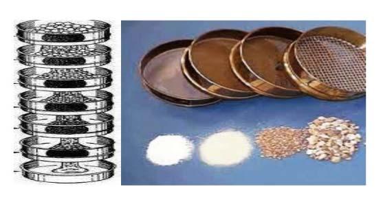
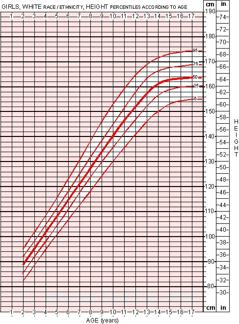
12 Example: Sieve Analysis Example: Growth Chart 12

13 Box and Whisker Plot: Box represents middle half of data, lower and upper quartiles Whiskers extend from box edges to minimum and maximum values (extremes) Dispersion represented by length of whiskers and box size Skew represented by relative position of mean and median within box, length of whiskers and position of 10 th and 90 th percentiles 13

14 Mean vs. Median Negative (Left) Skew Symmetric (No Skew) Positive (Right) Skew Example: Consider weights of n = 92 CEE students 14

15 Rank Weight Rank Weight Rank Weight Rank Weight Box Plot for Weight Data (n = 92) Comparative Box Plots: Men versus Women Men Women