Domestic Water Use and Piped Water Supply (PWS)

Transcription

1 Domestic Water Use and Piped Water Supply (PWS) Om Damani (Adapting from the slides of Milind Sohoni, Pooja Prasad, and Puru Kulkarni)

2 2

3 3

4 4

5 5

6 6

7 7

8 8

9 9

10 10

11 11

12 Agenda Introduction to Piped water schemes (PWS) Design of PWS Define demand Service level consideration Source identification ESR location and capacity design Pipe layouts ESR staging height and Pipe diameter Pump design Cost optimization 12

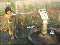
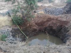
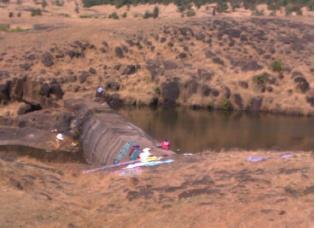
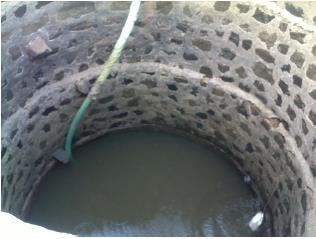
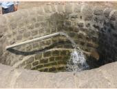
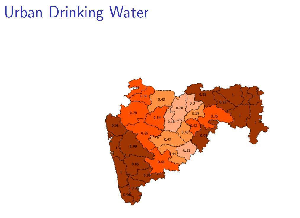
13 Water sources for different uses 13

14 The need for PWS Relevance of PWS Falling ground water levels drudgery removal, aspiration for many rural households, improved water quality in case of WTP GoI strategic goal to have 90% of all households with PWS by 2022 Currently at about 30% Source: NRDWP Strategic Plan , GoI 14

15 PWS Components Source Groundwater, surface water Transmission Network of pipes, tanks Delivery Public stand-posts, household taps 15

16 Typical Single Village PWSS 16

17 Multi village scheme (MVS) or Rural Regional scheme (RR) 17

18 Designing a PWS what does it entail? Pipe dia, type, length, layout Demand and service level Pump capacity Tanks: Number, location, mapping to demand, height, capacity Source 18

19 Design of a PWS scheme Characterize demand Identify habitations Population account for growth (ultimate stage population) account for cattle population LPCD norm for design (40/ 55/ 70/130 etc.) This gives us requirement for average daily demand from the source ultimate stage population * lpcd 19

20 Identify source options Musai Dolkhamb Kharade Adiwali Source: Analysis of tanker fed villages in Shahpur by Divyam Beniwal, Pallav Ranjan 20

21 Considerations for source identification Yield Will it meet the demand? Surface source: reservation for drinking water Ground water: Perform an yield test Water quality WTP required for a surface source Distance from target habitations Long distance => long pipelines => high investment cost high frictional losses & high leakages => hence, high recurring operational cost Elevation difference between source & target Big difference => high pumping cost (recurring) If source is at higher elevation => low operational cost 21

22 Design parameters depend on demand pattern 24x7 water service Water consump tion 4am 6am 8am 10am noon 2pm 4pm 6pm 8pm 10pm 12am 2am Intermittent service Water consump tion 4am 6am 8am 10am noon 2pm 4pm 6pm 8pm 10pm 12am 2am 22

23 How does service level impact asset design Total daily demand supplied in 2 hours => 12x increase in average outlet flowrate How does this impact Pipe diameter? ESR storage capacity? Pump capacity? In general, 24x7 service => lower asset cost compared to intermittent service 23

24 Flowrates Demand flow rate Variable for 24x7 supply: depends on consumption Intermittent supply: depends on designed service hours Supply flow rate Amount of water to be pumped (demand + x% leakages etc.) Pumping hours Depends on electricity outages ESRs help in meeting the demand flow rate while maintaining supply at a constant average flow rate 24

25 Example Ultimate stage population = 10,000 Demand = 10,000*50 lpcd = 50 m 3 per day Service Hours 24 hours service : Average demand flowrate = 50/24 m 3 /hr = 2.08 m 3 /hr Caution: this is average flow taken over service hours Pumping hours: Assume 10 hours Supply flow rate = 50 m 3 /10 hr= 5m 3 /hr in 10 hours 25

26 Example contd. Consumption is usually variable 24 hour service (variable demand) 10 hours of pumping (supply) 26

27 ESR Capacity Sizing Back to the Example Hour Demand Flow out Flow in Cumulative Balance % m3 m3 Balance 00:00 0% :00 0% :00 0% :00 0% :00 2% :00 5% :00 7% :00 10% :00 15% :00 15% :00 5% :00 2% :00 2% :00 1% :00 1% :00 2% :00 4% :00 8% :00 10% :00 7% :00 1% :00 1% :00 1% :00 1% ESR capacity 65 m3 Cumulative Balance Flow out m3 Flow in m3 Cumulative Balance 27

28 Benefits of ESRs Pump sizing for avg flow vs. max flow Water consump tion Max flow Avg flow 4am 6am 8am 10am noon 2pm 4pm 6pm 8pm 10pm 12am 2am Buffer capacity Peak consumption times Electricity outage Providing hydrostatic head 28

29 Location and count of ESRs Cluster based on Distance Elevation Population Practical considerations land availability Physical inspection required for accurate elevation data Source: North Karjat Feasibility Study by Vikram Vijay and team 29

30 Design of transmission network expected output Pipe layout, dia, type, length Pump capacity Tanks: Number, location, mapping to demand, height, capacity 30

31 Why MBR? MBR Master Balancing Reservoir Feeds the ESRs Holds additional x hours of buffer capacity Balances fluctuations in demand from ESRs against supply 31

32 Design of transmission network Pipe layout, dia, type, length Define residual head Pump capacity Tanks: height 32

33 Use of head in specifications Assume a column of water Pressure head at B = 100m Pressure at B = r* g* h = 1000 kg/m3*9.8 m/s2 * 100m = 980kPa Pressure depends on density of fluid Pressure at B for a column of mercury = kg/m3 *9.8 *100 = kpa A B A 100m P = 980 kpa 100m Easier to specify required head or discharge head instead of pressure -> no longer dependent on the fluid density B P = kpa 33

34 What is head? Hydraulic head: Total energy in a fluid Elevation head, pressure head, velocity head By Bernoulli s principle: Hydraulic head = elevation head+ pressure head + velocity head is constant B A h Pressure head at A = elevation head at B = rgh J Elevation head hs hp he K hs Pressure head datum o L Source: examples from Introducing Groundwater by Michael Price 34

35 Compute Residual Head at an Open Tap P 2 P 1 = ρgh 1 ρgh ρv 2 2 fhρg Hence you can calculate residual head Or discharge rate (Q) If you know the other f h = C*v = C*Q/A From itacanet.org Residual head non-zero at outlet: moving water zero at outlet: stationary 35

36 Residual heads in a Distribution Network Think of all the points where terms in Bernoulli equation will change 36

37 Design ESR staging height Define minimum residual head at delivery points 95m 100m X? 90m 88m Min Residual head = 5m Minimum required staging height depends on Elevation of supply / demand points Minimum residual head requirement and something else? 37

38 Frictional losses x Head loss y How does conservation of energy hold here? Water in Water out Total head loss (m of head loss/ km distance per m/s velocity) Pipe roughness Pipe length Flow rate Pipe diameter Pipe Roughness constant: Published for different materials Many models and empirical equations in literature to calculate head loss using this constant Source: example from Introducing Groundwater by Michael Price 38

39 Design ESR height 95m 100m >=95+5+z Z=head loss 90m 88m Min Residual head = 5m When can we use a GSR? Trade-off between pipe dia and tank staging height High staging height => low pipe diameter needed to achieve the same head why? Also implies higher pumping cost (Upstream impact recurring cost) 39

40 Pipe Types Pipe type usually driven by cost Most used types: PVC, GI (Galvanized Iron), HDPE (High density polyethylene), MDPE PVC: Most commonly used; low cost, easily installed. Prone to leakages, requires frequent maintenance GI: good for pipes installed over ground and can be easily welded but more expensive and prone to corrosion HDPE/MDPE: cheap, inert, comes in rolls of hundreds of meter, very low leakage. Electrofusion of joints requires expensive equipment; lower availability 40

41 Pipe Layout f1 f1+f2+f3 +f4+f5 A B f3+f4+f5 branches f1 C f5 f2 f3 f4 Branch network A B f2 Introducing a loop f1+f2+f3+ f4+f5 f3+f4+f5 branches C f5 f3 f4 Grid network 41

42 Example - Loops C 10 km A 1 m/s 10 km 10 km D B 1 m/s 1 m/s Frictional loss = 1m/ km per m/s velocity Branch velocity loss A-B 1m/s 10m C-A 2m/s 20m C-D 1m/s 10m C 10 km A 1 m/s 10 km 10 km D B 1 m/s 1 m/s Branch velocity loss A-B 0.5 m/s 5m C-A 1.5m/s 15m D-B 0.5m/s 5m C-D 1.5m/s 15m Introducing the loop reduced the ESR height requirement 42

43 Back to ESR height vs. pipe design Start with any reasonable ESR height List available options of {pipe dia, friction coeff, cost} For the given network and available pipe choices determine the optimal pipe choice for each branch such that the total pipe cost is minimized Optimization software such as Jaltantra/Loop may be used for this 43

44 Back to ESR height vs. pipe design Lowest investment Is the operational cost acceptable? 44

45 Pump specs Pump power is proportional to Q*r*g*h Q supply flow rate h differential head between pump and MBR (static head + frictional head + velocity head) r fluid density; 45

46 JalTantra for Optimization of Village Piped Water Schemes

47 Issues in Design and Implementation of MVS A Vicious Cycle Technical Problems Financial Hit to Scheme Scheme Starts Failing Villagers Pull Out

48 Problem Formulation Input: List of (village id, location, population) Source of water Links connecting the nodes Cost per unit length for different pipe diameters Output: For each link, length of different pipe diameters to be used Optimization Objective : Capital Cost of Pipes

49 Minimum pressure required = 5m Pipe roughness = 140 Commercial pipe info: Example Network Diameter Source Head: 100m 1 3 Elevation: 70m Demand: 5 lps Unit Cost m 500m Elevation: 80m Demand: 2 lps 2 700m 4 Elevation: 50m Demand: 3 lps Optimization 1 141m + 859m 500m 3 Head: 5m Head: 15.42m 2 579m + 121m 4 Head: 5m Diameter Length Cost k k k TOTAL COST 776.9k

50 General Formulation for Piped Water Network Cost Optimization Number of links Objective Cost: NL NP i=1 j=1 C(D j )l ij Number of commercial pipes Length of j th pipe of i th link Unit cost of j th pipe Node Constraint: Min. pressure reqd. at node n P n H R E n Head of source node Elevation of node n NP i S n j=1 Links from source to node n Unit headloss of j th pipe of i th link HL ij l ij Pipe Constraint: Unit Headloss: NP j=1 l ij = L i Total length of i th link HL ij = flow i roughness j 4.87 diameter j

51 Future Work Immediate Tasks Web Application GIS Integration Usability Features Medium term Pressure Rating Pressure Reducing Valves Pumps ESR Elevation Operational Cost Long term Multiple Sources Looped Network Cost Allocation ESR Location

52 Sample GIS Integration for Input Data Web based Application that runs Google Earth. Navigate to the region of interest using Google Earth. Mark the nodes by traversing a path for the network. Inter node distance and the elevation of nodes is displayed on the screen. When the user submits the data, it is formatted as JalTantra Input file.

53 JalTantra vs. EPANET Note: Network layout required for both. In general Use JalTantra for design: it optimizes pipe diameters (but only if the network is branched and gravity-fed) Use EPANET for simulation if the system has pumps, valves, loops, and time-variations in demand or supply

54 JalTantra input/output For every node For every pipe Elevation Demand Min residual pressure Pipe length Pipe roughness Existing/Planned JalTantra DESIGN output: Lowest pipe diameters Cost per pipe and total piping cost For the network Network layout Source HGL Diameter options Min & Max head loss/km SIMULATION output: Flow in each pipe Pressure at each node Head-loss in each pipe Head loss formula

55 EPANET input/output For every node For every pipe Elevation Demand Pipe length Pipe roughness Pipe diameter EPANET SIMULATION output: Pressure at each node Velocity in the pipe Head-loss in each pipe Network layout Source details Extended time simulation For the network Demand/supply schedule Details of pumps, valves and tanks Units (SI or Imperial) Head loss formula

56 Example network layout Junction Elev m 1 ESR Elev HGL 120 m Pipe # 1 L 1000 m 2 3 Pipe # 3 L 400 m Pipe # 2 L 300 m 4 Demand Node Elev m Village Pop Demand Node Elev m Village Pop. 600

57 Demand calculation Rural supply norm: 55 lpcd Assume the source is an ESR which will supply the full day s water in 6 hours Demand (lps) = pop. * 55 lpcd/(6 hr * 3600 s/hr) Node 3 => 600 * 55/(6*3600) = 1.5 lps Node 4 => 1200 * 55/(6*3600) = 3.0 lps

58 1 Pipe # 1 2 L 1000 m Pipe # 2 4 L 300 m Node Data Pipe # 3 L 400 m 3 Pipe Data Commercial Pipe Data JalTantra input

59 JalTantra output Node Results Pipe Results Cost Results

60 HGL vs. Total pipe cost and Pipe 1 diameter /180 mm Total Pipe Cost ( x Rs ) mm 110/125 mm 90/110 mm 90/110 mm HGL of source (m) Increasing the source HGL often reduces total piping cost

61 EPANET What does EPANET do? Public domain software for simulation of water distribution networks EPANET analyses the flow of water in each pipe, the pressure at each node, the height of water in a network. Advantages: 1. Extended period hydraulic analysis for any system size. 2. Simulation of varying water demand, constant or variable speed pumps, and the minor head losses for bends and fittings. 3. EPANET can compute the energy consumption and cost of a pump. 4. Can model various valve types - pressure regulating, and flow control valves 5. Provides a good visual depiction of the hydraulic network 6. Data can but imported in several ways the network can be drawn and data can be imported from Google Earth. 7. Water quality-simulation of chlorine concentration in each pipe and at each node.

62 EPANET slide 1 ( set up) Source Reservoir Pipe 1 Node 2 Pipe 2 Pipe 3 Node 4 Node 3

63 EPANET Output file- Nodes EPANET Output file- Pipes

64 Extended period analysis EPANET Time Pattern: To make our network more realistic for analyzing an extended period of operation we will create a Time Pattern that makes demands at the nodes vary in a periodic way over the course of a day. The variability in demands can be addressed through multipliers of the Base Demand at each node. Nodal demands, reservoir heads, pump schedules can all have time patterns associated with them. As an example of how time patterns work consider a junction node with an average demand of 3 lps. Assume that the time pattern interval has been set to 4 hours and a pattern with the following multipliers has been specified for demand at this node- Time Period Multiplier Then during the simulation the actual demand exerted at this node will be as follows: Hours Demand

65 References Mokhada MVS design report: TR-CSE pdf Khardi Rural Piped Water Scheme TR-CSE pdf North Karjat RR scheme feasibility study: Sugave MVS scheme analysis: Tadwadi SVS scheme failure analysis 65