GIS as a Tool for Assisting TMDL Development

Transcription

1 GIS as a Tool for Assisting TMDL Development by Reem Zoun Jon Goodall Tim Whiteaker David Maidment, Ph.D. Center for Research in Water Resources University of Texas at Austin July 10, 2003

2 Outline Overview Bacteria Monitoring Data Analysis Introduction to Model Builder Introduction to Schematic Network Processing Modeling Bacteria Transport to Bay Results

3

4 TMDL Requirements for Oyster Water Use Water Quality Criteria for Fecal Coliform Median Fecal Coliform concentration in bay and gulf waters shall not exceed 14 colonies per 100 ml or 14 MPN. No more than 10% of all samples should exceed 43 colonies per 100 ml.

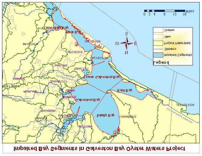
5 Potential Sources of Contamination Point Sources: Wastewater treatment plans and sewer overflows Rivers and streams entering the estuary Non-Point Sources: Storm-water runoff from adjacent watersheds Bird droppings Marinas and boats

6 Research Objective of the Galveston Bay Oyster Water Project 1. Compile and analyze existing monitoring data 2. Create a GIS based model to predict the mean concentration observed in the bay

7 Outline Overview Bacteria Monitoring Data Analysis Introduction to Model Builder Introduction to Schematic Network Processing Modeling Bacteria Transport to Bay Results

8

9 Statistical Distribution of TDH Monitoring Data

10 Profile of Mean FC concentration along streams

11 Outline Overview Bacteria Monitoring Data Analysis Introduction to Model Builder Introduction to Schematic Network Processing Modeling Bacteria Transport to Bay Results

12 Introduction to Model Builder Tool Output Data Input Data Note: Model Builder will be available in ArcGIS 9

13 Outline Overview Bacteria Monitoring Data Analysis Introduction to Model Builder Introduction to Schematic Network Processing Modeling Bacteria Transport to Bay Results

14 Introduction to Schematic Network Processing Start: Point and Nonpoint source loads End: Load Estimate for every link and node Applications: 1. Long-term pollutant load estimations 2. Rainfall/Runoff flow routing

15 Outline Overview Bacteria Monitoring Data Analysis Introduction to Model Builder Introduction to Schematic Network Processing Modeling Bacteria Transport to Bay Results

16 Land to water delivery Input: Nonpoint source load Output: Bay concentration CSTR Along river transport C = C o e -kt Input: Bird load River outlet to bay delivery

17

18 Component 1

19 Land Use EMC table (cfu/m 3 ) EMC grid (cfu/m3) + = Component 1: Calculating Expected Mean Concentration (EMC) of bacteria in number of coliform units per cubic meter of water (C)

20 Component 1

21 Component 1 Component 2

22 Precipitation (mm/yr) Conversion factor (m 3 /mm) Runoff (m 3 /yr) x C(P) = Component 2: Calculating runoff in cubic meters per year per grid cell (Q)

23 Component 1 Component 2

24 Component 2 Component 1 Component 3

25 EMC grid (cfu/m3) Runoff (m 3 /yr) Load (cfu/yr) x = Component 3: Calculating bacteria load per grid cell (L)

26 Component 2 Component 1 Component 3

27 Component 4 Component 2 Component 1 Component 3

28 Runoff grid(m 3 /yr) Runoff on Watersheds (m 3 /yr) Load grid (cfu/yr) Load on Watersheds (cfu/yr) Load on SchemaNodes (m 3 /yr) and Component 4: Summarizing runoff and load on Watershed and SchemaNode features

29 Component 4 Component 2 Component 1 Component 3

30 Component 4 Component 2 Component 1 Component 3 Component 5

31 Schematic Network Predicted Total Load LinkType 1: Land to Water 2: Along River 3: River to Bay Bacteria Loads Bay Conc. (cfu/m 3 ) Load flux (cfu/yr) Component 5: Calculating the total accumulated load of bacteria transport through the schematic network by using the Schematic Network Processing tool

32 Outline Overview Bacteria Monitoring Data Analysis Introduction to Model Builder Introduction to Schematic Network Processing Modeling Bacteria Transport to Bay Results

33 Bacteria Loads Bay Conc. (cfu/m 3 ) Load flux (cfu/yr)

34 Comparison of Results Mean Concentration (cfu/ml) Automated Thesis Observed 0 Upper Galveston Bay Trinity Bay East Bay West Bay Chocolate Bay Lower Galveston Bay

35 Acknowledgement Dr. Barbara Moore, University of Texas at San Antonio Fred Kopfler, Gulf of Mexico Program Sandra Alvarado, Texas Commission on Environmental Quality Dr. George Ward, UT Austin Dr. Neal Armstrong, UT Austin Gary Heideman, Texas Department of Health

36 Questions?

37 Fecal Coliform Bacteria The total coliform (TC) bacterial group is a large group of anaerobic, gram-negative, nonspore-forming, rod-shaped bacteria. Fecal coliform bacteria, which belong to this group, are present in large numbers in the feces and intestinal tracts of humans and other warm-blooded animals. The presence of fecal coliform bacteria in aquatic environments indicates contamination with the fecal material of humans or other animals. Shellfish species reside in estuaries where fecal microbes can enter their tissues as they feed by filtering water to gather nutrients. Properly cooked shellfish pose no threat of infectious disease, but oysters, which are frequently consumed raw, may hold potentially pathogenic bacteria or viruses for weeks or months before harvest.

38 Classification of Molluscan Shellfish Growing Areas Texas Department of Health administers classification of molluscan shellfish growing areas to regulate oyster harvesting from the impaired segments.

39

40

41

42

43 Profile of Mean FC concentration along streams

44 Profile of Mean FC concentration along Streams

45 Watersheds Draining to Galveston Bay

46 Database Development and Arc Hydro for Study Area

47 Residence time in Lake Houston Watersheds Draining to Lake Houston In order to account for the retention of fecal coliform in Lake Houston, residence time in the lake is added to travel times of outflows from the watersheds located upstream of Lake Houston. Residence time, td = V / Q = m3 / 60.2 m3 / sec = days where V is the volume of the lake and Q is flow rate.

48 Decayed Annual Fecal Colirom Load with and without Retention in Lake Houston

49 Estimation of Avian Load The loading is computed at each location as: Load from Gull = Number of breeding pairs 2 Amount of excretion per bird FC concentration in bird dropping percent of FC reaching the bay

50 Marinas, WQP, Sludge and Sewage

51 Load Allocation in the Impaired Bay Segments 3.5E E+16 Fecal Coliform Loading (cfu/yr) 2.5E E E E+16 Adjacent Non-Point Load (cfu/yr) Upstream Non-Point Load (cfu/yr) Point Source Load (cfu/yr) Load from Laughing Gull (cfu/yr) Load from Lake (cfu/yr) 5.0E E+00 Upper Trinity Bay Galveston Bay (2421) (2422) East Bay (2423) Bay Segment West Bay (2424) Chocolate Bay (2432) Lower Galveston Bay (2439)

52 Consolidation and Accumulation of Decayed Load Decayed fecal coliform loads are summed at all the watershed outlets and the stream end points using the Consolidate Attribute tool in the Attribute Tools of ArcHydro toolset. The consolidated loads are then accumulated to the HydroJunctions located at the edges of the impaired bay segments

53 Total Load Allocation Adjacent Non-Point Load (cfu/yr) Upstream Non-Point Load (cfu/yr) Load from Lake (cfu/yr) Point Source Load (cfu/yr) Load from Laughing Gull (cfu/yr)

54 Land-use Categories in Study Area Source: 1990 USGS land use and land cover data.

55 Expected Mean Cconcentration Table Expected Mean Concentration

56 EMC Grid Expected Mean Concentration Land-use EMC Grid

57 Runoff from Precipitation Data Expected Runoff Equation: Q =0.51*P Precipitation Runoff, Q Runoff Precipitation, P Source: Spatial Water Balance of Texas by S Reed,S.M., D.R. Maidment, and J. Patoux

58 Loading Estimation Approach Runoff EMC Grid Non-Point Load Load Mass = EMC * Runoff

59 Decaying Non-point Load from Upstream Watersheds = 0 x c c exp KB U c = concentration at the inlet of the waterbody c 0 = concentration at watershed outlet x = downstream length from watershed outlet U =flow velocity Load = Flow *c

60 Conclusion Findings from Data Analysis: The monitoring dataset shows several high concentration zones of fecal coliform in the study area. Proximity is important in identifying the sources of contamination as the causes and effects are local. Typical concentrations of bacteria in runoff waters in the drainage area of the bay are much larger than those found in the bay waters. Inactivation (caused by salinity and sunlight) of bacteria is a key role in analysis. Estimation of Loadings: A regional GIS model is presented for estimation of non-point fecal coliform loadings from adjacent and upstream watersheds. A CSTR model accounting for the total loadings and decay of bacteria in the bay gives a bay concentration of fecal coliform in the same magnitude as the observed one. Non-point loadings from upstream watersheds represented the largest contributor of fecal coliform in Galveston Bay. Retention in upstream watershed segments should significantly lower loadings to the bay segments. Estimated fecal coliform loadings from Laughing Gull populations showed significant contributions to West Bay and Lower Galveston Bay.

61 Fecal Coliform Input from Bird Droppings Estimation of fecal coliform input from birds: Species and number of birds Distribution birds Level of FC in different species FC conc. and amount of waste/time Point of fecal deposition shore or water

62 Estimation of Total Loadings

63 Continuous Stirred Tank Reactor (CSTR) Model The model assumes complete mixing of the waste load in the entire body of water and steady state condition. The computation accounts for only non-point load. W Concentration, c = Q + K Where, W is pollutant load, Q is runoff volume, KB is the overall net first order decay rate and V is the volume of water body. B V

64 Comparison of Modeled Concentration to Observed Concentration CSTR Concentration (cfu/100ml) TDH Geometric Mean of Observed Data (cfu/100ml) % Difference TCEQ % Difference Upper Galveston Bay (2421) % Trinity Bay (2422) % % East Bay (2423) % 3.7 3% West Bay (2424) % 5.9 2% Chocolate Bay (2432) Lower Galveston Bay (2439) % The value obtained from the model is in the same magnitude as the observed values which is a reasonable value given the degree of spatial variability in bacterial concentration in the bay segment demonstrated earlier.