Prepared by the Capital Area Council of Governments Air Quality Program. September 4, 2015

Transcription

1 CAPCOG FY14-15 PGA FY14-1 Deliverable Amendment 1 Prepared by the Capital Area Council of Governments Air Quality Program September 4, 2015 PREPARED UNDER A GRANT FROM THE TEXAS COMMISSION ON ENVIRONMENTAL QUALITY The preparation of this report was financed through grants from the State of Texas through the Texas Commission on Environmental quality. The content, findings, opinions, and conclusions are the work of the author(s) and do not necessarily represent findings, opinions, or conclusions of the TCEQ. Page 1 of 57

2 CAPCOG Photochemical Modeling Analysis Report, September 4, 2015 Table of Contents 1 Introduction Analysis of Existing Photochemical Modeling Studies Projections of Future Ozone Design Values Review of AACOG s 2018 Modeling Projections Review of EPA s Tier 3 Vehicle and Fuel Standard Modeling Projections Review of EPA s 2008 Ozone NAAQS Transport Modeling Projections Review of EPA s 2014 Ozone NAAQS Proposal Modeling Projections Summary Modeling Projection Analysis Analysis of Background Ozone Levels and Ozone Transport UT s Zero-Out Modeling for the EAC SIP UT s APCA Analysis for the 2006 Base Case EPA s 2008 Ozone NAAQS Transport Modeling Sensitivity and Control Strategy Modeling UT Early Action Compact SIP Modeling UT 2006 and 2007 Modeling of Ozone Impact of Proposed New Power Plants UT 8-O3 Flex Plan 12-Point Source APCA Modeling UT and AACOG Texas Lehigh Modeling UT 2006 Base Case Sensitivity Modeling AACOG 2012 and 2018 Eagle Ford Shale Modeling AACOG COTA Major Event Modeling EPA 2014 Ozone NAAQS Proposal Modeling New Photochemical Modeling Runs for Control Strategy Analysis Texas Lehigh Emission Reductions I-M Program Emission Reductions Conclusions & Recommendations Appendix A: QA Summary Appendix B: AACOG Modeling Report Table 1. Relative reduction factors calculated for 2013 AACOG modeling scenarios... 9 Table 2. Adjusted baseline and future design values based on AACOG's 2013 modeling incorporating 2014 monitoring data... 9 Page 2 of 57

3 CAPCOG Photochemical Modeling Analysis Report, September 4, 2015 Table 3. Key design value modeling ratios derived from Tier 3 photochemical modeling Table 4. Synthesized design value projections for (ppb) Table 5. Modeled impacts from zero-out modeling in EAC SIP (ppb ozone) Table 6. APCA modeling for June 2006 base case average for top 4 modeled peak 8-hour ozone averages (ppb) Table 7. Ozone contributions from EPA 2018 interstate transport ozone modeling (ppb) Table 8. Ozone contribution from EPA 2017 interstate transport ozone modeling (ppb) Table 9. Average daily NO X emissions from wildfires in 2011 by month and county (tons per day) Table 10. EAC SIP control strategy and sensitivity modeling Table 11. Calculated EAC SIP NOX and VOC sensitivities Table 12. Sensitivity calculated for Austin-Round Rock MSA zero-out run Table 13. Modeled impact of a 6.46 tpd NO X reduction at Oak Grove (ppb) Table 14. NO X Emissions at 12 plants modeled by UT in 2010 (tons per day) Table 15. Calculated average peak 8-hour ozone sensitivity to NO X emissions from 12 local point sources in UT 8-O3 Flex modeling for the four highest 8-hour ozone levels (ppb/tpd NO X ) Table 16. Estimated average local point source NO X emission contributions to peak 8-hour ozone concentrations, 2013 (ppb) Table 17. Average sensitivity of peak 8-hour ozone to VOC emissions from 12 local point sources (ppb/tpd VOC) Table 18. Average contribution of biogenic emissions to peak ozone levels in EAC SIP modeling and seasonal modeling (ppb) Table 19. Calculated sensitivities from AACOG modeling of Texas Lehigh emission reduction impacts (ppb/tpd NOX) Table 20. Seasonal model ozone impacts at CAMS 3 from Texas Lehigh modeled by UT (ppb) Table 21. Average NO X and VOC sensitivities calculated from UT's June 2006 sensitivity analysis for days with top 4 ozone levels (ppb/tpd) Table 22. Modeled impact of post-2006 emission reductions at Alcoa/Sandow Table 23. Modeled impact on peak 8-hour ozone concentrations on days when peak modeled 8-hour ozone averages exceeded 70 ppb within the Austin-Round Rock MSA (ppb) Table 24. NO X and VOC emissions sensitivities and VOC-to-NO X ratio Table 25. Average Eagle Ford Shale NO X Sensitivities (ppb/tpd of NO X -equivalents) Table 26. Daily NO X and VOC emissions estimates for simulated major event at COTA, 2012 (tons per day) Table 27. Change in peak 8-hour ozone averages due to major events at COTA and calculated sensitivities Table 28. Sensitivities calculated from EPA's ozone NAAQS proposal modeling (ppb/tpd) Table 29. Comparison of NO X emissions estimates in Clean Power Plan proposal and final rulemakings (thousand tons) Table 30. Baseline and adjusted Texas Lehigh hourly emissions in 2015 modeling analysis (tons of NO X )50 Table 31. Summary of ozone impacts from Texas Lehigh NOX reductions from 9 am - 3 pm Table 32. Average ozone impact and sensitivity to Texas Lehigh NOX emission reduction program on June 2006 Ozone Action Days Page 3 of 57

4 CAPCOG Photochemical Modeling Analysis Report, September 4, 2015 Table 33. Modeled emissions changes due to I-M program in Table 34. Average modeled peak 8-hour ozone change and NO X sensitivities for I-M program Table 35. Estimated avg. impact of I-M program on peak 8-hour ozone levels, 2018 (ppb) Figure 1. AACOG's 2018 projected ozone design values at CAMS 3 and 38 (ppb)... 7 Figure 2. Comparison of AACOG Eagle Ford drilling projection to actual permits issued Figure 3. Comparison of AACOG Eagle Ford oil production projection to actual production Figure 4. Comparison of AACOG Eagle Ford gas production projection to actual production Figure 5. Comparison of AACOG Eagle Ford condensate production projection to actual production Figure 6. Updated projected ozone design values using AACOG modeling and 2014 monitoring data and CAPCOG Updates Figure 7. Estimated likelihood that the Austin-Round Rock MSA would attain a 65 ppb standard in 2016 and 2017 using AACOG modeling projections and monitoring data Figure 8. Estimated likelihood that the Austin-Round Rock MSA would attain a 70 ppb standard in 2016 and 2017 using AACOG modeling projections and monitoring data for all growth scenarios Figure 9. Tier 3 standard modeling projected design values for Travis County Figure 10. EPA design value projections for interstate transport for the 2008 ozone NAAQS (ppb) Figure 11. Interpolated ozone design values (ppb) for using EPA's ozone NAAQS proposal modeling Figure 12. Composite of Travis County monitored and projected design values Figure 13. UT 2006 base case APCA source regions Figure 14. Comparison of the impact of biogenic emissions on CAMS 3 and 38 in EPA ozone transport modeling (ppb) Figure 15. Impacts of SNCR at CAMS 3 (Murchison) by hour of the day in UT 2010 modeling Figure 16. Geographic regions used in EPA's 2014 Ozone NAAQS Proposal Modeling Figure 17. Modeled 2025 ozone design values based on EPA's sensitivity modeling (ppb) Figure 18. Comparison of impact of across-the board NO X emission reductions to I-M program NOX reductions (ppb/tpd) Page 4 of 57

5 CAPCOG Photochemical Modeling Analysis Report, September 4, Introduction This report provides a secondary analysis of existing photochemical modeling data that is available for Central Texas and new photochemical modeling data and analysis estimating the impact on peak ozone levels from two local emission reduction strategies. These analyses should help provide an improved understanding of the area s likely future ozone design values and the sensitivity of local ozone levels to various regional emission reductions. For the secondary analysis of existing photochemical modeling data, CAPCOG staff reviewed a wide range of existing studies and data applicable to the region, including: Early Action Compact (EAC) State Implementation Plan (SIP) photochemical modeling conducted by the University of Texas at Austin (UT) in 2003; An Anthropogenic Precursor Culpability Assessment (APCA) analyses of local point source contributions to peak 8-hour ozone levels conducted by UT in 2009; A Performance evaluation of the June 2006 base case conducted by UT in 2012; APCA and sensitivity studies of the June 2006 base case conducted by UT in 2012; 2012 and 2018 modeling conducted by the Alamo Area Council of Governments (AACOG) using the June 2006 base case completed in 2013; Modeling the ozone impact of major events at the Circuit of the Americas (COTA) completed in 2014; EPA modeling for the Tier 3 light-duty vehicle and fuel standards completed in 2013 and 2014; EPA modeling of 2025 ozone levels for its proposal to revise the National Ambient Air Quality Standards (NAAQS) for ground-level ozone completed in 2014; EPA modeling of 2017 and 2018 ozone levels for use in analyzing cross-state ozone impacts for the 2008 ozone NAAQS completed in By performing a synthesized analysis across all of these studies, CAPCOG was able to develop a broad understanding of what these existing studies can tell us about the relative contribution of different regions to local ozone levels, the sensitivity of local ozone levels to changes in emissions, and the expected future ozone levels for The new photochemical modeling completed for this project involves evaluating: 1. the modeled impacts of the vehicle emissions inspection and maintenance (I-M) program implemented in Travis and Williamson County on peak 8-hour ozone levels in 2012, and 2. the modeled impact of Texas Lehigh s voluntary ozone action day NO X emission control program on peak ozone levels. For both of these analyses, prior photochemical modeling work had estimated the impacts of these programs using older photochemical modeling platforms based on projected emissions reductions. By analyzing the impacts of these emission reduction programs on local ozone levels using historical data for 2012 and using a more up-to-date modeling platform, this project should provide a clearer picture of the benefits of these efforts and the extent to which they are contributing to reductions in local ozone levels. Page 5 of 57

6 CAPCOG Photochemical Modeling Analysis Report, September 4, Analysis of Existing Photochemical Modeling Studies 2.1 Projections of Future Ozone Design Values Some of the key questions that stakeholders in the local air quality planning are facing require an understanding of where the region s ozone levels are likely to be from This is particularly important for understanding: 1. The likelihood that the area would be designated nonattainment for EPA s proposed ozone NAAQS; 2. The likelihood that the area would miss the attainment date for a Marginal area if designated nonattainment without further emission reductions; 3. The likelihood that the area would miss the attainment date for a Moderate area if designated nonattainment without further emission reductions; 4. The likely date that the area would attain the proposed standard without further local emission reduction measures being implemented; and 5. Whether the area s ozone levels would be able to meet an even lower possible standard of 60 ppb within this timeframe without further local emission reductions. There are four sets of modeling results that CAPCOG used in order to evaluate the range of possible projected ozone design values for this period, including: AACOG s 2013 modeling of the 2012 and 2018 ozone levels using the June 2006 base case modeling platform; EPA s modeling for the proposal and final rulemaking package for the Tier 3 light-duty vehicle and fuel standards, which includes 2005 and 2007 base cases, and projections for 2017, 2018, and 2030 with and without these controls; EPA s modeling for the 2008 ozone NAAQS interstate transport impacts, which use a 2011 base case and include projections to 2017 and 2018; and EPA s modeling for the proposed 2015 ozone NAAQS based on a 2011 base case and 2025 projections, including a series of sensitivities Review of AACOG s 2018 Modeling Projections In 2013, AACOG completed photochemical modeling for CAPCOG that involved using updated emissions inputs based for projections AACOG had already made for 2012 and 2018 using the June 2006 base case. 1 These modeling runs included three different scenarios for 2012 and 2018 different scenarios for 2018: 2012 scenario: o A baseline scenario based on existing TCEQ emissions projections for 2012 from prior SIP work for the Dallas-Fort Worth (DFW) area; o An updated baseline scenario that incorporated the emissions inventory estimates from AACOG s Eagle Ford shale oil and gas emissions inventory; and 1 Body_Only.pdf Page 6 of 57

7 8-Hour Ozone Design Value (ppb) CAPCOG Photochemical Modeling Analysis Report, September 4, 2015 o An updated baseline scenario that incorporated both AACOG s Eagle Ford Shale emissions estimates and updates CAPCOG made to the local emissions inventories in the 10-county CAPCOG region, which includes Bastrop, Blanco, Burnet, Caldwell, Fayette, Hays, Lee, Llano, Travis, and Williamson Counties, plus Milam County; 2018 scenario: o A future baseline scenario based on existing TCEQ emissions projections for 2018 from prior SIP work for the Houston-Galveston-Brazoria (HGB) area; o An updated future baseline scenario that incorporated the emissions inventory estimates from AACOG s Eagle Ford shale oil and gas emissions inventory using a low-growth projection; o An updated future baseline scenario that incorporated the emissions inventory estimates from AACOG s Eagle Ford shale oil and gas emissions inventory using a moderate-growth projection; o An updated future baseline scenario that incorporated the emissions inventory estimates from AACOG s Eagle Ford shale oil and gas emissions inventory using a high-growth projection; and o An updated future baseline scenario that incorporated the emissions inventory estimates from AACOG s Eagle Ford shale oil and gas emissions inventory using a moderate-growth projection and CAPCOG s emissions inventory updates for the 10-county CAPCOG region (Bastrop, Blanco, Burnet, Caldwell, Fayette, Hays, Lee, Llano, Travis, and Williamson) plus Milam Counties. These projections do not account for emission reductions in the on-road sector due to the Tier 3 vehicle and fuel standards that will start to occur in 2017, to some degree, they would reflect an uncontrolled 2018 scenario, so the actual design values would be expected to be lower in Figure 1. AACOG's 2018 projected ozone design values at CAMS 3 and 38 (ppb) CAMS 3 CAMS Baseline 2018 Baseline w/eagle Ford Shale Low Growth 2018 Baseline w/eagle Ford Shale Moderate Growth 2018 Baseline w/eagle Ford Shale High Growth 2018 Baseline w/eagle Ford Shale Moderate Growth & CAPCOG Updates Page 7 of 57

8 CAPCOG Photochemical Modeling Analysis Report, September 4, 2015 Since a region s ozone design value is based on the highest design value at any monitor within the region, these results indicate that the region s design value in 2018 would be parts per billion (ppb), since the design value truncates any fractions of a ppb. This would put the region s ozone levels below the level of the current 75 ppb standard and below the highest level of the ppb range proposed by EPA, but above the lower level of the range. AACOG s design value projections applied the modeled relative reduction factors for each monitoring station to a 2012 modeling baseline design value that was calculated according to the following equation: This baseline design value differed from the standard approach, which would have also included 2014 monitoring data, since the modeling took place in 2013 and the 2014 monitoring data was not yet available. Based on the data for CAMS 3 and CAMS 38, AACOG calculated a baseline design value of 73.0 ppb for both stations. CAPCOG then calculated the relative reduction factors (RRFs) for each 2018 scenario modeled by dividing the projected design values reported in Figure 5-1 in AACOG s report by AACOG s calculated baseline design value. Since AACOG s results included the moderate growth scenario both with and within CAPCOG s updates, CAPCOG also calculated what the approximate RRFs for the low and high growth scenarios would be if they had incorporated the CAPCOG emissions inventory updates. The following equations show the calculations used for each scenario for CAMS 3. The following table provides a summary of the RRFs calculated for CAMS 3 and 38 for each scenario, including the adjusted low and moderate RRFs to account for the impact of CAPCOG s emissions inventory updates. Page 8 of 57

9 CAPCOG Photochemical Modeling Analysis Report, September 4, 2015 Table 1. Relative reduction factors calculated for 2013 AACOG modeling scenarios Scenario CAMS 3 CAMS Baseline Baseline, Eagle Ford Low Growth Baseline, Eagle Ford Mod. Growth Baseline, Eagle Ford High Growth Baseline, Eagle Ford Mod. Growth + CAPCOG Updates Baseline, Eagle Ford Low Growth + CAPCOG Updates Baseline, Eagle Ford High Growth + CAPCOG Updates Since 2014 monitoring data is now available, CAPCOG updated the 2012 baseline design values as follows: Next, CAPCOG applied the RRFs in Table 1 to the updated baseline design values in order to obtain updated projections for 2018 under each scenario. The updated baseline and projected design values are shown in Table 2 below. Table 2. Adjusted baseline and future design values based on AACOG's 2013 modeling incorporating 2014 monitoring data Scenario CAMS 3 CAMS Baseline Baseline Baseline, Eagle Ford Low Growth Baseline, Eagle Ford Mod. Growth Baseline, Eagle Ford High Growth Baseline, Eagle Ford Mod. Growth + CAPCOG Updates Baseline, Eagle Ford Low Growth + CAPCOG Updates Baseline, Eagle Ford High Growth + CAPCOG Updates Among these three growth scenarios, it is possible to compare AACOG s projections to actual drilling and production data since 2012 in order to evaluate which scenario is most likely. Figures 2 5 below show the projected and actual permitting and production data for , based on Railroad Commission Data 2 and AACOG s 2013 Eagle Ford Emissions Inventory Page 9 of 57

10 CAPCOG Photochemical Modeling Analysis Report, September 4, 2015 Figure 2. Comparison of AACOG Eagle Ford drilling projection to actual permits issued Low Projection (Wells Drilled Per Day) Moderate Projection (Wells Drilled Per Day) High Projection (Wells Drilled Per Day) Actual Permits Issued Per Day The comparison of the number of permits issued to the number of wells drilled per day shows that there were more permits being issued between than there were wells being drilled, but the number of permits issued per day fell down to the level of drilling consistent with the low projection. 4 Texas Railroad Commission. Texas Eagle Ford Shale Drilling Permits Issued 2008 Through July /6/2015. Available online at: (Retrieved 9/4/2015) reflects January July. Page 10 of 57

11 Barrels Per Day CAPCOG Photochemical Modeling Analysis Report, September 4, 2015 Figure 3. Comparison of AACOG Eagle Ford oil production projection to actual production ,500,000 2,000,000 1,500,000 1,000,000 Low Projection Moderate Projection High Projection Actual 500, For oil production, even though the total number of new drilling permits has dropped off significantly since 2014 due to low oil prices, the oil production level in 2015 has stayed about the same as 2014, which itself was higher than the high growth scenario. This discrepancy between drilling activity and production reflects the fact that many wells have already been drilled that are not yet producing, and that the marginal costs of producing oil from an existing well would be lower than the total cost if drilling the well in the first place was considered. As long as marginal revenue from producing the oil exceeds the marginal cost of bringing the well s production online, it would still make economic sense to produce and sell the oil from existing wells, even if it doesn t make economic sense to drill new ones. Based on the 2015 level, it is likely that oil production levels will be closer to the moderate growth scenario than either the high or low growth scenario. If production levels stayed constant to 2015 levels, the levels for would be between the low and moderate growth scenarios. 5 Texas Railroad Commission. Texas Eagle Ford Shale Oil Production 2008 through June /21/2015. Available online at (Retrieved 9/4/2015) reflects January June. Page 11 of 57

12 MMCF Per Day CAPCOG Photochemical Modeling Analysis Report, September 4, 2015 Figure 4. Comparison of AACOG Eagle Ford gas production projection to actual production ,000 7,000 6,000 5,000 4,000 3,000 Low Projection Moderate Projection High Projection Actual 2,000 1, Similar to oil production, gas production has leveled off between 2014 and 2015, even increasing a bit, despite the large drop in drilling permits. For the same reasons that the oil production is likely to remain high for some time, gas production is also likely to remain high through Unlike oil production, however, the gas production levels are significantly higher than all three of AACOG s projections and if production levels stayed constant to 2015 levels, the levels for would be between the high and moderate growth scenarios. 6 Texas Railroad Commission. Texas Eagle Ford Shale Total Natural Gas Production 2008 through June /21/2015. Available online at Retrieved 9/4/ reflects January June. Page 12 of 57

13 Barrels Per Day CAPCOG Photochemical Modeling Analysis Report, September 4, 2015 Figure 5. Comparison of AACOG Eagle Ford condensate production projection to actual production , , , , ,000 Low Projection Moderate Projection High Projection Actual 100, Condensate production from also exceeded all three of AACOG s projections, but 2015 levels are just below AACOG s high projection. If production levels stayed even for , production would be higher than the moderate projection for 2016 and 2017, but below the moderate projection for These data provide a mixed picture as to what to expect for While new drilling has dropped off significantly, production has simply leveled off, and may not decrease for some time even with the price of oil as low as it is since many existing wells have not yet been brought online. Nevertheless, since there is only a 0.3 ppb difference between the low and high projection, it is not likely that the growth or a reduction in production in the Eagle Ford Shale would have a significant policy-relevant impact on the area s design values in A significant amount of the projected impacts are already baked in to the 2012 baseline design value, so the relatively difference in the projections does not represent the total impact from Eagle Ford Shale emissions on ozone design values, just the difference in various growth assumptions. For a full discussion of the impact of Eagle Ford Shale emissions on the 2012 baseline, see Section Using the 2012 baseline design value and the 2018 projections, it is possible to interpolate design values for intermediate years. This method of estimating the design values implicitly assumes that the change between these years would be linear. While this method would not directly account for the 7 Texas Railroad Commission. Texas Eagle Ford Shale Condensate Production 2008 through June /21/2015. Available online at Retrieved 9/4/ reflects January June. Page 13 of 57

14 Design Value (ppb) CAPCOG Photochemical Modeling Analysis Report, September 4, 2015 fact that the actual changes in emissions that CAPCOG expects to occur between these two years are likely to be front-loaded to the earlier portion of this period, the projection time frame is short enough, and the long-run trend in ozone design value changes from 1999 to 2014 shows a fairly linear pattern, CAPCOG believes that this method is appropriate for the general planning purposes that this analysis is being used for. If anything, CAPCOG expects that this method would slightly over-estimate design values in these intermediate years, with a larger magnitude of over-estimation earlier during this time frame. Figure 6 shows the adjusted design value projections using each of the three Eagle Ford growth scenarios with the CAPCOG emissions inventory updates (modeled for the moderate scenario, calculated for the low and high growth scenarios, as described above). The error bars represent the % difference between the maximum and minimum design values in the period relative to the weighted average used for the baseline design value calculation. For , these represented -5.3% on the low end and +3.1% on the high end to reflect the range for CAMS 3, which was the modeled peak ozone monitor for all years other than The smaller error bars in 2012 reflect the range of design values for CAMS 38, since that had a higher weighted average design value than CAMS 3 (71.8 ppb). Figure 6. Updated projected ozone design values using AACOG modeling and 2014 monitoring data and CAPCOG Updates Low + CAPCOG Moderate + CAPCOG High + CAPCOG Notably, these interpolations provide an accurate design value for 2014 (69 ppb), and match the region s current 2015 design value based on monitoring data collected through September 4 th (68 ppb at both monitors). In neither 2016 nor 2017, years that could be used as the basis for the area s nonattainment designation, would the difference in these projections for low or high growth Page 14 of 57

15 CAPCOG Photochemical Modeling Analysis Report, September 4, 2015 scenarios make a particularly policy-relevant difference in the ozone levels. As these data show, the difference between the design value projections for the low and high growth scenarios is only 0.3 ppb in 2018, since much of the existing impact from Eagle Ford emissions is already accounted for in the 2012 baseline. Using the projected design values in Table 2, CAPCOG estimated the likelihood that the area s 2016 and 2017 design values would measure attainment of a 65 ppb standard, which using the truncation allowed by EPA, could be as high as 65.9 ppb. CAPCOG calculated the likelihood of attaining the standard as follows: While the 2012 and 2018 projected design values more nearly resemble the 4 th highest daily peak 8- hour ozone average in a given year than the actual design value, as mentioned earlier, the interpolated design values calculated above have matched the region s actual 2014 design value and the 2015 design value through September Figure 7. Estimated likelihood that the Austin-Round Rock MSA would attain a 65 ppb standard in 2016 and 2017 using AACOG modeling projections and monitoring data Low + CAPCOG Moderate + CAPCOG High + CAPCOG 57% 55% 52% 34% 33% 31% This analysis was repeated for evaluation against a 70ppb standard and shown below. Because all projections predicted design values below 70 ppb by 2016, the likelihood of attaining a 70 ppb standard would be 100% across for all scenarios using this method. Page 15 of 57

16 CAPCOG Photochemical Modeling Analysis Report, September 4, 2015 Figure 8. Estimated likelihood that the Austin-Round Rock MSA would attain a 70 ppb standard in 2016 and 2017 using AACOG modeling projections and monitoring data for all growth scenarios Low + CAPCOG Moderate + CAPCOG High + CAPCOG 100% 100% 100% 100% 100% 100% Again, since these modeling data do not reflect the impact of the Tier 3 vehicle standards, which would result in a higher probability that the area would be able to measure attainment of the standard in 2017 than this modeling would reflect. What these analyses show is that: 1. It is more likely than not that the area s 2016 design value will be above a 65 ppb standard; 2. There is still a significant chance that the 2016 and 2017 design values could be low enough to reach attainment of a 65 ppb standard and possibly enable the area to avoid a nonattainment designation; 3. There is a very high likelihood that the area s 2016 and 2017 design values will be below a 70 ppb standard, even with the significantly higher ozone levels measured in the region in 2015 than had been measured in 2013 or 2014; and 4. The area s design value is likely to be close enough to a 65 ppb standard that additional emission reductions and stepped-up efforts to scrutinize monitoring data for exceptional events in 2016 could make the difference in the region s attainment status Review of EPA s Tier 3 Vehicle and Fuel Standard Modeling Projections In 2013 and 2014, the EPA completed photochemical modeling in support of the Tier 3 light-duty vehicle and fuel standards that included controlled and uncontrolled design value projections to 2017, 2018, and The proposal included modeling using a 2005 base year, a 2017 projection year, and a 2030 Page 16 of 57

17 Ozone Design Value (ppb) CAPCOG Photochemical Modeling Analysis Report, September 4, 2015 projection year. 8 The final included modeling using a 2007 base year, a 2018 projection year, and a 2030 projection year. 9 Figure 9. Tier 3 standard modeling projected design values for Travis County Proposal Final Both the proposal and final modeling shows a ppb or more in ozone reductions between the base year and the uncontrolled intermediate projection year (1.1 ppb per year in the proposal, 1.0 ppb in the final. The proposal showed a 0.71 ppb reduction in ozone design values in 2017 between the uncontrolled and controlled scenario (a 1.05% reduction), while the final showed a 0.63 ppb reduction in 2018 between the uncontrolled and controlled scenario (a 0.96% reduction). Between the controlled scenarios in the intermediate year and the final year, the proposal modeling showed an average annual reduction of 0.46 ppb, while the final modeling showed an average annual reduction of 0.29 ppb. In addition to being directly useful for projections for these years, the modeling data is also useful for understanding the relative reductions between these years, since these relative reductions can be applied to other modeling analyses like the AACOG modeling in order to estimate what the modeled impact of the Tier 3 standards on the AACOG modeling data would be. The table below shows some of the key ratios calculated for these purposes. Table 3. Key design value modeling ratios derived from Tier 3 photochemical modeling Modeling Analysis Design Value Ratio Description Ratio Proposal 2017 Controlled / 2017 Uncontrolled Proposal 2030 Controlled / 2017 Controlled Page 17 of 57

18 CAPCOG Photochemical Modeling Analysis Report, September 4, 2015 Modeling Analysis Design Value Ratio Description Ratio Final 2018 Controlled / 2018 Uncontrolled Final 2030 Controlled / 2018 Controlled Review of EPA s 2008 Ozone NAAQS Transport Modeling Projections In 2015, EPA completed modeling projections to 2017 and 2018 based on its 2011 modeling platform in order to provide data to states to assist them in implementing the good neighbor provisions of the Clean Air Act. The baseline design values for the period were 73.7 ppb at CAMS 3 and 72.0 ppb at CAMS 38. EPA s initial set of projections was released in February 2015, and showed projected design values of 67.7 ppb at CAMS 3 and 65.2 ppb at CAMS EPA released updated modeling in July 2015 that showed projected design values of 67.8 ppb at CAMS 3 and 65.5 ppb at CAMS 38 in to The modeling showed annual reductions of 0.9 ppb at CAMS 3 and 1.0 ppb over this time period, while the modeling showed annual reductions of 1.0 ppb at CAMS 3 and 1.1 ppb at CAMS 38. Figure 10. EPA design value projections for interstate transport for the 2008 ozone NAAQS (ppb) CAMS 3 CAMS Baseline 2017 Projection (Jul. 2015) 2018 Projection (Feb. 2015) Review of EPA s 2014 Ozone NAAQS Proposal Modeling Projections EPA s regulatory impact analysis (RIA) for its 2014 ozone NAAQS proposal includes photochemical modeling based on a 2011 modeling platform with projections to The base case modeling included a projection that accounted for all existing rules, and showed projected 2025 design values of 65.7 ppb at CAMS 3 and 63.1 ppb at CAMS 38. The estimated baseline design value for 2025 also incorporated emission reductions from EPA s Clean Power Plan and emission reductions needed to Page 18 of 57

19 CAPCOG Photochemical Modeling Analysis Report, September 4, 2015 bring the Houston and Dallas-Fort Worth areas into attainment of the current 75 ppb standard. The projected design values incorporating the Clean Power Plan emission reductions were 64.9 ppb and 62.2 ppb for CAMS 3 and CAMS 38, respectively, reductions of ppb. Beyond these, EPA used an explicit emission reduction scenario for Texas, scaling back the total emissions needed to bring into attainment of the standard based on the sensitivity of the key monitors to the emission reductions included in the model. EPA then applied these adjusted emission reductions to the sensitivities calculated for each monitor in order to calculate the incremental ozone reductions that would be expected at these monitors from reducing emissions just enough to enable the Houston and Dallas-Fort Worth areas to model attainment of the 75 ppb standard in EPA s reported design value for Travis County using these methods was 64 ppb, but did not report this number out to tenths of a ppb. 12 Using an explanation and a spreadsheet of modeling results EPA provided to CAPCOG via , CAPCOG calculated the estimated design value for the region. First, CAPCOG identified the monitors in the Houston and Dallas-Fort Worth that were modeled to still be violating the 2008 ozone NAAQS in the modeling sensitivity that incorporated the Clean Power Plan emissions reductions. These monitoring stations were: Station in Brazoria County: 76.6 ppb; and Station in Tarrant County: 76.0 ppb. In order to reach attainment, the Brazoria County monitor s modeled design value needed to be reduced by 0.7 ppb in order to reach 75.9 ppb, which gets truncated to a 75 ppb design value. Based on its 1.4 ppb response to 102,770 tons of explicit annual NO X emission reductions in the sensitivity 7 scenario, CAPCOG calculated that it would take 51,712 tons of NO X reductions beyond the Clean Power Plan reductions in order to achieve the 0.7 ppb reduction needed at the Brazoria County monitor. By multiplying these emission reductions to the sensitivities for CAMS 3 and CAMS 38, CAPCOG calculated that these emission reductions would achieve a 0.7 ppb reduction for CAMS 3 and a 0.5 ppb reduction for CAMS 38. These reductions would produce an overall design value of 64.3 ppb for the region, based on CAMS 3 s design value. Eq. 1 Eq Page 19 of 57

20 CAPCOG Photochemical Modeling Analysis Report, September 4, 2015 Eq. 3 Eq. 4 Eq. 5 These projections suggest that if there are not new NO X controls in Texas beyond those that the Clean Power Plan and the implementation of the 75 ppb standard, Travis County would face the possibility that it might continue to be in violation of a 65 ppb standard beyond the attainment date for Marginal areas. Figure 11 shows interpolated design values between the 2011baseline, as identified in the transport modeling projections and this 2025 projection. This simple interpolation shows a 2023 attainment year. While many of the emission reductions and hence the ozone reductions are projected to be more pronounced during the earlier years of this period, which would make incremental changes in design values smaller in the later years, this projection still suggests that there is a risk that the area s ozone levels may not decrease enough between now and 2019 in order to attain a 65 ppb standard by the expected attainment deadline for Marginal areas. Figure 11. Interpolated ozone design values (ppb) for using EPA's ozone NAAQS proposal modeling Page 20 of 57

21 CAPCOG Photochemical Modeling Analysis Report, September 4, Summary Modeling Projection Analysis While there are strengths and weaknesses to each individual modeling study for forecasting future design values, a meta-analysis across all of these studies can help even out the variability due to selection of model and emissions inventory projection assumptions. This synthesis helps the overall analysis benefit from the strengths of each study and compensate for their weaknesses, thereby enabling a more robust overall picture of likely future ozone levels. Figure 12 below shows the monitored design values for Travis County, as well as the following: The weighted baseline design value used by EPA for the 2008 ozone NAAQS modeling and the 2014 ozone NAAQS proposal modeling; The weighted baseline design value used to adjust the AACOG modeling projections as described in section 2.1.1; The 2017 controlled projection from the Tier 3 proposal modeling; The 2017 projection from the July 2015 EPA ozone transport modeling; The 2018 projection from the February 2015 EPA ozone transport modeling; The 2018 controlled projection from the Tier 3 final modeling; The adjusted 2018 AACOG projection using the moderate Eagle Ford growth and CAPCOG updates scenario (0.990 adjustment to reflect impact of Tier 3 standards modeled in final rulemaking); The adjusted 2018 projection using the high Eagle Ford growth scenario (also (0.990 adjustment to reflect impact of Tier 3 standards modeled in final rulemaking); EPA s calculated 2025 projected design value, accounting for the impacts of the Clean Power Plan and emission reductions needed to bring Houston and the Dallas-Fort Worth area into attainment of the 2008 ozone NAAQS; The 2030 projection from the Tier 3 proposal modeling; and The 2030 projection from the Tier 3 final modeling. Page 21 of 57

22 Ozone Design Value (ppb) CAPCOG Photochemical Modeling Analysis Report, September 4, 2015 Figure 12. Composite of Travis County monitored and projected design values Modeled Monitored Linear (Modeled) y = x R² = 0.83 The following table shows a comparison of projected design values for each year from , using three different methods: Method 1a (2011 base case, 2011 baseline); o 2011 Base Case photochemical model; o center-weighted baseline DV; o 2017 projected DV in July 2015 O 3 Transport modeling; o 2025 projected DV in O3 NAAQS proposal; o 2030 projection using Tier 3 final 2030 controlled divided by interpolation of 2025 DV; o Interpolations for , , and ; Method 1b (2011 base case, 2012 baseline); o Same as method 1a, except using a center-weighted design value and the relative differences between each year and 2012; Method 2 (2006 base case, 2012 baseline): o June 2006 Base Case photochemical model; o AACOG 2012 and 2018 emissions scenarios; o center-weighted baseline design value; o Interpolated design values for ; o Reduction in 2017 and 2018 projections based on Tier 3 vehicle standards reduction factor for impact of Tier 3 standards on Travis County design value; Page 22 of 57

23 CAPCOG Photochemical Modeling Analysis Report, September 4, 2015 o Projection to 2025 using ratio of EPA s 2025 projected design value for Travis County to EPA s 2008 ozone transport modeling (July release) design value for 2017; o Interpolated design values for ; o Projection to 2030 using 2018 estimated design value multiplied by ratio of 2030 Tier 3 controlled DV to 2018 Tier 3 DV; and o Interpolated DVs for Table 4. Synthesized design value projections for (ppb) Year 2011BC/2011BL 2011BC/2012BL 2006BC/2012BL Since these projections are based on four different base case scenarios (2005, June 2006, 2007, and 2011) and several different sets of emissions assumptions, they provide a unique opportunity to take advantage of multiple different sets of analyses in order to get an idea of where the region s ozone levels are likely to be in some key future years. Some key insights from this analysis include There is a chance that the Travis County monitors could have ozone design values that are in attainment of an ozone standard set at 65 ppb, but it is more likely than not that it would be above that level; There are multiple estimates that show attainment of a 65 ppb standard by the end of 2018; The overall trend suggests attainment of a 65 ppb standard by the end of 2020 or 2021; If, in the review that will be due by the end of 2020, EPA were to set the standard at 60 ppb, the lowest level recommended by CASAC in the current review, the region may still not be in attainment of a standard that low by Page 23 of 57

24 Tyler Dallas Houston Corpus Christi Victoria San Antonio Austin Missouri Louisiana Texas CAPCOG Photochemical Modeling Analysis Report, September 4, Analysis of Background Ozone Levels and Ozone Transport Another important piece of information that air quality planners need is the extent to which an area s peak ozone levels are influences by background concentrations and pollution transported into the area. The studies that this section analyzes include: UT s zero-out modeling for the EAC SIP; UT s APCA analysis for the June 2006 base case modeling episode; EPA s modeling for the Cross-State Air Pollution Rule (CSAPR); and EPA s 2008 ozone NAAQS transport modeling. Caution should be used in comparing these results, since they were all based on different modeling platforms and include different meteorological and chemical models. The EAC SIP modeling in particular is now 12 years old and is mainly useful compare the scientific understanding of ozone formation has changed over time UT s Zero-Out Modeling for the EAC SIP The University of Texas s modeling for the EAC SIP included zero-out modeling analyses showing the impacts of anthropogenic emissions from Texas, Louisiana, Missouri, and the Austin, San Antonio, Victoria, Corpus Christi, Houston, Dallas, and Tyler areas on peak 8-hour ozone concentrations modeled for These results are summarized in the table below. Table 5. Modeled impacts from zero-out modeling in EAC SIP (ppb ozone) Day 9/15/ /16/ /17/ /18/ /19/ /20/ TOTAL Among other things, these data showed a significant impact on local ozone levels from Louisiana on all episode days, a significant impact from Missouri on three days, a significant impact from Houston on three days, and a significant impact from the Tyler area on one day. The Austin-Round Rock MSA s contribution of only 7.7 ppb indicates that it was contributing one third of the state s total contribution to peak ozone levels, and only 9% of peak 8-hour ozone levels overall See tables 5a and 5b. Page 24 of 57

25 CAPCOG Photochemical Modeling Analysis Report, September 4, UT s APCA Analysis for the 2006 Base Case UT conducted an anthropogenic precursor culpability assessment (APCA) modeling analysis of the June 2006 base case in 2012 that divided TCEQ s 4 km x 4 km grid system into the following sources: 14 initial conditions: boundary conditions; Austin-Round Rock Area-1; Beaumont/Port Arthur Area-2; Corpus Christi-3; Dallas/Fort Worth-4; Houston/Galveston/Brazoria-5; Tyler/Longview/Marshall-6; San Antonio-7; Waco-8; Victoria-9; Northeast Texas-10; East Texas-11; South Texas-12; West Texas-13; Central Texas power plants (all emissions in the 4-km grid cells that contain the Freestone, Big Brown, Limestone County, Twin Oaks, Tenaska in Grimes County, and Gibbons Creek Plants).-14; Central Texas-15; Louisiana-16; All other geographic areas within the modeling domain-17; Bell County-18; Burnet County-19; Fayette County-20; Lee County-21; and Milam County Page 25 of 57

26 CAPCOG Photochemical Modeling Analysis Report, September 4, 2015 Figure 13. UT 2006 base case APCA source regions Page 26 of 57

27 CAPCOG Photochemical Modeling Analysis Report, September 4, 2015 Table 6. APCA modeling for June 2006 base case average for top 4 modeled peak 8-hour ozone averages (ppb) APCA Source Regions C3 % of Total C38 % of Total Austin-Round Rock MSA % % Milam County % % Lee County % % Fayette County % % Bell County % % Burnet County % % HGB nonattainment area % % DFW nonattainment area % % Beaumont-Port Arthur area % % Tyler-Longview-Marshall area % % Waco area % % Corpus Christi area % % Victoria area % % San Antonio-New Braunfels MSA % % Northeast-rural % % East-rural % % South-rural % % West-rural % % Central Texas power plants % % Central-rural % % Louisiana (LA) % % Geographic areas except TX/LA % % Boundary and initial conditions % % Total predicted ozone % % UT s modeling showed: Almost half of the Austin-Round Rock MSA s ozone levels were attributable to boundary conditions and areas outside of Texas. o Boundary and initial conditions were responsible for about a quarter of peak ozone levels. o Louisiana s contribution to peak ozone levels in the Austin-Round Rock MSA are high enough that its major sources could be considered to be significantly contributing to nonattainment or interfering with maintenance of EPA s proposed ozone standard in violation of Section 110 of the Clean Air Act, which would be grounds for local governments or the state filing a Section 126 petition with the EPA. Another quarter of peak ozone concentrations is coming from areas in Texas outside of the Austin- Round Rock MSA. o With the exception of the DFW nonattainment area, the Waco area, and Bell County, all major metropolitan areas in the eastern portion of the state contributed 0.65 ppb or more to one or both of the Austin regulatory ozone monitors, which is enough that the area s would pass EPA s air quality contribution screen for assessing interstate impacts (1% of the NAAQS) for the lowest level of EPA s proposed ozone standard. Page 27 of 57

28 CAPCOG Photochemical Modeling Analysis Report, September 4, 2015 o o o The Houston area s contributions to peak ozone levels in the Austin-Round Rock MSA are particularly notable this suggests that emission reductions in recent years may have played a significant role in reducing ozone levels in the Austin-Round Rock area, but the area s contributions likely remain quite significant. The rural areas of the state that were modeled also each contributed more than 0.65 ppb; The impact of the group of the Central Texas power plants modeled was less than 0.65 ppb, and represented only 9-10% of the total impact from emissions within this source region. Each of the adjacent counties does not typically have a major impact on ozone levels individually, but they can have substantial impacts on ozone levels within the region on certain high ozone days, and collectively contribute a significant amount on most days. o On all days > 75 ppb, these counties had collective impacts of 0.09 ppb to 5.31 ppb at CAMS 3 and 0.09 ppb to 8.22 ppb on CAMS 38. o The average contribution of Burnet County on CAMS 38 s peak ozone levels includes one day with an exceptionally high contribution of 6.61 ppb and another day with a 1.27 ppb contribution (June 14 th and 28 th ) on all other days >75 ppb, the average contribution was 0.26 ppb. On these same days, the contribution at CAMS 3 was 0.44 ppb and 2.57 ppb. There was another day with modeled 8-hour ozone over 75 ppb when Burnet County s emissions contributed 2.5 ppb (June 3 rd ). These contributions indicate that while Burnet County s emissions usually won t have a significant impact on peak ozone levels, they can occasionally be a significant factor. o The average contribution of Milam County to peak ozone levels at CAMS 3 was heavily influenced by one day when the impact was 3.2 ppb (June 13 th ). This day was not among CAMS 38 s top four modeled ozone concentrations, so it was not included in the average listed above, but Milam County contributed 6.09 ppb to peak ozone at CAMS 38 on that day, and it contributed 1.06 ppb to another day with ozone levels over 75 ppb (June 3 rd ); for all days over 75 ppb, the average contribution of Milam County to peak ozone levels is actually higher at CAMS 38 (0.84 ppb) than at CAMS 3 (0.46 ppb). While Milam County s emissions don t frequently contribute much to high ozone levels in the region, when the wind is blowing from that direction, the impact can be quite substantial. o Similar to the data for Burnet and Milam County, Bell County s contributions are not often a significant factor in peak ozone levels at CAMS 3 or CAMS 38, but can have a significant impact on certain days. Bell County s emissions contributed 2.54 ppb to peak ozone at CAMS 3 on June 14 th and 0.92 ppb on June 28 th, but was no more than 0.15 ppb on all other days over 75 ppb. At CAMS 38, Bell County s emissions contributed 0.74 and 0.71 ppb on these same days, and on all other days over 75 ppb, the contribution was no more than 0.28 ppb. The higher impact on CAMS 3 relative to CAMS 38 may reflect the importance of on-road emissions along interstate highway 35 on Bell County s contributions to ozone formation. o Fayette County s contributions at CAMS 3 and 38 were higher than 0.65 ppb on only one day in the episode June 9 th, when the impacts were 1.19 ppb and 0.94 ppb at each monitor, respectively. Aside from that day, the average was only 0.24 for CAMS 3 and 0.26 for CAMS 38. o Lee County had a large impact on peak ozone at CAMS 38 on only one day 1.13 ppb, but had a tiny impact on CAMS 38 all other days over 75 ppb and a very small impact on CAMS 3 on all days modeled. The Austin-Round Rock MSA s contribution to peak ozone levels tends to be substantially higher on the top four ozone days than on the next 5-9 highest days; o While emissions from the Austin-Round Rock MSA contributed ppb to peak 8-hour ozone concentrations at CAMS 38 on the top four modeled days, and ppb to the top four days at Page 28 of 57

29 CAPCOG Photochemical Modeling Analysis Report, September 4, 2015 o CAMS 3, the average for the next 5 highest days was 5.29 ppb lower at CAMS 38 and 5.52 ppb lower at CAMS 3; This suggests that there is a higher sensitivity to local emissions on the four worst ozone days that would be important for the region s ozone design value than there would be for all days when ozone levels are moderate or worse EPA s 2008 Ozone NAAQS Transport Modeling In January 2015, EPA released APCA modeling showing the estimated impacts of interstate air pollution, boundary conditions, biogenic emissions, and other sources (Canada, Mexico, fires, and offshore sources) on peak ozone levels across the country. 15 This analysis used EPA s 2011v6.1 platform projected to The table below shows the modeled impact of states with an average impact of 0.50 ppb or more, as well as the contributions from tribal areas, other sources. A state with an impact at that level would be more likely than not to cause the area s design value to be 1 ppb higher than it would have been without that state s contributions, so it provides a statistical basis for considering its contribution significant. For the EPA s Cross-State Air Pollution Rule (CSAPR), it used 1% of the NAAQS as a threshold for further analyzing a state s contribution as possibly being significant. Table 7. Ozone contributions from EPA 2018 interstate transport ozone modeling (ppb) Source Region/Type CAMS CAMS Alabama Arkansas Illinois Louisiana Missouri Oklahoma Texas Other States Tribal Canada, Mexico, Offshore, Fires Biogenic Emissions Boundary Conditions Predicted Design Value A court ruling in December required EPA to move up the attainment year when ozone levels would need to be in compliance with the 2008 ozone NAAQS, so in July 2015, EPA released another set of modeling using a 2017 analysis year. 17 The modeling was based on an updated emissions inventory platform, and therefore produced somewhat different interstate contributions than what would have been expected from simply modeling one year earlier. Between these two years, 2017 is a more relevant Page 29 of 57

30 CAPCOG Photochemical Modeling Analysis Report, September 4, 2015 year for the Austin-Round Rock area since EPA has the ability to incorporate 2017 monitoring into its nonattainment designation process if it extends the process from two years after the standard is set to three years after as allowed under the Clean Air Act. Table 8. Ozone contribution from EPA 2017 interstate transport ozone modeling (ppb) Source Region/Type CAMS CAMS Alabama Arkansas Illinois Louisiana Missouri Oklahoma Texas Other States Tribal Canada and Mexico Offshore Fires Biogenic Emissions Boundary Conditions Predicted Design Value Both sets of results show that total anthropogenic emissions from within the U.S. is expected to contribute ppb peak ozone levels in 2017/2018, meaning that only about 40%-45% of the peak ozone levels that the Austin-Round Rock area would be experiencing would be controllable through the SIP process at that point. Of that, 8-10 ppb would be attributable to interstate air pollution. About 4 ppb of the interstate contribution is attributable to states with impacts of 0.5 ppb or more. Over half of that impact comes from just one state Louisiana. Subtracting these interstate impacts leaves only about 30% of peak ozone levels that could be controlled through Texas s SIP process. Based on the relative contribution of the Austin-Round Rock MSA to the rest of Texas in UT s APCA modeling for the 2006 base case, this means that the Austin area s contribution is likely to be approximately 8-10 ppb, which is only 10-15% of the modeled ozone levels for those years. The impacts of the other sources, which include Canada and Mexico, offshore, fire, and biogenic emissions are also notable. While these sources were grouped together in EPA s 2018 modeling, they were separately modeled in the 2017 modeling. Offshore sources include marine-going vessels and offshore oil platforms both of which the federal government has jurisdiction over. The contributions of these sources on peak ozone levels are quite significant enough so that their contributions could be the large enough to keep the area from being able to measure attainment of EPA s proposed ozone standard for the period EPA is likely to use as the basis for nonattainment designations. The modeled impact of fires was even more significant, and likely reflects the exceptionally bad wildfires that occurred throughout the state and especially in Central Texas in As the table below shows, the average daily NO X emissions from wildfires that EPA modeled for Page 30 of 57

31 CAPCOG Photochemical Modeling Analysis Report, September 4, 2015 the 2017 scenario, based on the base case 2011 emissions. 18 All of the four highest 8-hour ozone averages at CAMS 3 in 2011 occurred from August 28 through September 20. According to EPA s documentation, the 2011 emissions are day-specific. 19 Table 9. Average daily NO X emissions from wildfires in 2011 by month and county (tons per day) Month Bastrop Caldwell Hays Travis Williamson Total January February March April May June July August September October November December Annual Considering the abnormally high local wildfire emissions levels in 2011 and the modeled impact based on these emissions, it is likely that the actual impact in a typical year would be much lower enough so that the 2017 modeled design value would likely be low enough to be in attainment of the EPA s proposed ozone standard if it set as low as 65 ppb. Biogenic emissions also play a significant role in modeled peak ozone levels, and the impact changed substantially between the EPA s 2018 modeling and its subsequent 2017 modeling. The modeled impact changed by almost 2 ppb between these two modeling scenarios, as the figure below shows. 18 ftp://ftp.epa.gov/emisinventory/2011v6/v2platform/reports/2017eh_county_monthly_report.xlsx 19 Page 31 of 57

32 CAPCOG Photochemical Modeling Analysis Report, September 4, 2015 Figure 14. Comparison of the impact of biogenic emissions on CAMS 3 and 38 in EPA ozone transport modeling (ppb) 2018 Modeling 2017 Modeling CAMS 3 CAMS 38 Documentation for EPA s ozone transport modeling for the 2008 ozone NAAQS can be found at Sensitivity and Control Strategy Modeling This section provides a review of the sensitivity and control strategy modeling for the region dating back to the EAC SIP. As was discussed in the previous section, caution should be used in comparing these results, since they are based on different modeling platforms and include different meteorological and chemical models. The EAC SIP modeling in particular is now 12 years old, and is based on emissions models, chemical models, and meteorological models that have since been superseded by more advanced techniques. However, these older results are still useful in comparing the scientific understanding of ozone formation has changed over time and in understanding the relative impacts of different geographic areas and control strategies to one another UT Early Action Compact SIP Modeling The photochemical modeling that UT performed for the Austin-Round Rock area as part of the EAC SIP included a series of modeling runs testing the sensitivity of local ozone levels to changes in local NO X and VOC emissions. These analyses were based on a September 1999 modeling episode, Carbon Bond 4 (CB4) chemistry, MM5 meteorology, and a 2007 projection year. They included both broad sensitivity analyses and control strategy modeling Page 32 of 57

33 Table 10. EAC SIP control strategy and sensitivity modeling CAPCOG FY14-15 PGA FY14-1 Deliverable Amendment 1 Scenario I/M Program: Travis and Williamson I/M Hays Stationary Point Source Controls Area Source VOC Controls Low RVP Gasoline TERP Additional Mobile Source Controls 21 Alcoa Reductions Baseline NO X Δ (tpd) VOC Δ (tpd) DV (ppb) 21 TERMS, Commute Solutions, Heavy Duty Idling Restrictions 22 Calculated using Page 33 of 57

34 CAPCOG FY14-15 PGA FY14-1 Deliverable Amendment 1 By isolating the impacts modeled for just the scenarios in which only NO X or only VOC emission changes occurred, CAPCOG calculated the sensitivities show in the table below. Since scenario 6 involves a change in NO X only relative to Scenario 5, CAPCOG also calculated the sensitivity for that scenario incremental to the design value modeled for Scenario 5. Table 11. Calculated EAC SIP NOX and VOC sensitivities Scenario Emission Source Pollutant Response (Δ ppb/δ tpd) 2 Point Sources NO X Area and Mobile Sources VOC On-Road and Non-Road Mobile NO X Alcoa Reductions Only NO X Point Sources VOC Using an average of the two NO X reduction scenarios for MSA-only reductions, the average sensitivity for NO X would be ppb per tpd NO X emissions from within the MSA, while the average sensitivity for VOC would be ppb per tpd VOC emissions from within the MSA (a VOC sensitivity to NOX sensitivity ratio of 0.26). This indicates that it would take about 3.86 tpd VOC reductions to achieve the same ozone reduction impact as 1 tpd of NO X reductions from within the region. The data for the Alcoa reductions indicate that there would need just under 2 tpd of NO X reductions at Alcoa in order to achieve the same ozone reduction as a 1 tpd reduction in NO X emissions from within the MSA. UT s zero-out modeling also enabled calculation of overall sensitivity of peak 8-hour ozone concentrations to emissions reductions within the Austin-Round Rock MSA. Using the day-specific anthropogenic VOC and NOX emissions modeled, 23 along with the 0.26 ratio of VOC sensitivity to NOX sensitivity, CAPCOG calculated the sensitivities for the zero-out Austin-Round Rock MSA run in terms of ppb of ozone to tpd of NOX-equivalents. Table 12. Sensitivity calculated for Austin-Round Rock MSA zero-out run Episode Day NO X (tpd) VOC (tpd) VOC to NO X sensitivity Ratio NO X - equivalents (tpd) Austin Zero- Out Impact (ppb) Sensitivity (ppb/tpd NO X - equivalents) 9/15/ /16/ /17/ /18/ /19/ /20/ Avg Page 34 of 57

35 CAPCOG Photochemical Modeling Analysis Report, September 4, UT 2006 and 2007 Modeling of Ozone Impact of Proposed New Power Plants In 2006 and 2007, UT completed modeling showing the potential impact of several proposed coal-fired power plants across the state on Austin-area ozone levels. 24 This analysis involved preparing an updated 2007 future case based on the Early Action Compact SIP modeling and then adding the proposed power plants into the model to measure the change in modeled ozone levels. For this secondary analysis, the most useful comparisons are between Runs 4 and 5 as described below: Run 3: Modified 2007 Future Case, which removed three Alcoa boilers (located in Milam County, which lies just outside the 10-county CAPCOG region and northeast of the Austin-Round Rock MSA) that were shut down after 2006 and updated point source emissions from other existing point sources; Run 4: Modified 2007 Future Case with tpd NO X at each of Oak Grove Power Plant s 2 units (located in Robertson County northeast of the Austin-Round Rock MSA) and tpd at Sandow 5 (reduced from tpd in run 3); Run 5: Modified 2007 Future Case with tpd NOX at each of Oak Grove s 2 units and tpd at Sandow 5. The differences in emissions and modeled peak 8-hour ozone averages between Run 4 and Run 5 ( tpd NO X at Oak Grove) enabled CAPCOG to calculate the sensitivity of CAMS 3 and 38 to Oak Grove s NO X emissions. Table 13. Modeled impact of a 6.46 tpd NO X reduction at Oak Grove (ppb) Date CAMS 3 CAMS 38 9/ / / / / / Avg Based on these responses, CAPCOG calculated the average sensitivities to NOX emissions at Oak Grove: CAMS 3: ppb O 3 /tpd NO X CAMS 38: ppb O 3 /tpd NO X Based on the facility s 2013 annual emissions of 4, tons of NO X reported to TCEQ, the estimated impact of this facility would now expected to be 0.02 ppb at CAMS 38 and 0.01 ppb at CAMS 3 if meteorology were similar to the September 1999 episode. 24 McGaughey, Gary; Alba Webb; Cyril Durrenberger, Elena McDonald-Buller, and David T. Allen. Assessing the Air Quality Impacts in the Austin area Associated with the Proposed Operation of Eight New Coal-Fired Power Plants in Texas. Prepared by the University of Texas at Austin for the Capital Area Council of Governments. March 30, Page 35 of 57

36 CAPCOG Photochemical Modeling Analysis Report, September 4, UT 8-O3 Flex Plan 12-Point Source APCA Modeling In 2010, UT conducted two sets of APCA modeling that evaluated the impacts of 12 point source NO X emissions in the Austin-Round Rock MSA, Fayette County, and Milam County. These modeling analyses were based on the TCEQ s 4 km x 4 km September 1999 modeling platform (September 13, 1999 September 20, 1999) projected to 2007 that was used for the EAC SIP and the EPA s 12 km x 12 km 2002 seasonal modeling platform (June 1, 2002 September 30, 2002). 25 The 2002 model used the Community Multiscale for Air Quality (CMAQ) model and CB5 chemistry. Receptors included: 1. 5-County Max: the MSA grid cell with the maximum 8-hour ozone concentration each day; 2. Audubon: 3 x 3 12 km grid cells surrounding and including the Audubon (C38) monitor; 3. Murchison: 3 x 3 12 km grid cells surrounding and including the Murchison (C3) monitor; and 4. Downtown Austin: 3 x 3 12 km grid cells surrounding and including the grid cell centered on downtown Austin. Sources modeled included: 1. Initial Conditions NO X ; 2. Boundary Conditions NO X ; 3. Biogenic NO X ; 4. Fayette Power Project (RN ) NO X ; 5. Sandow (RN /RN ) NO X ; 6. Decker (RN ) NO X ; 7. Texas Lehigh (RN ) NO X ; 8. Sim Gideon (RN ) NO X ; 9. Lost Pines (RN ) NO X ; 10. Bastrop Energy Center (RN ) NO X ; 11. Hays Energy Center (RN ) NO X ; 12. UT Hal Weaver Power Plant (RN ) NO X ; 13. Sand Hill (RN ) NO X ; 14. Austin White Lime (RN ) NO X ; 15. Prairie Lea (RN ) NO X ; 16. Total NO X emissions from all other point sources in domain; 17. Total NO X emissions from all other area sources in domain; 18. Initial Conditions VOC; 19. Boundary Conditions VOC; 20. Biogenic VOC; Source VOC Total; 22. Total VOC emissions from all other point sources in domain; and 23. Total VOC emissions from all area sources in domain. In general, UT used the 2007 emissions inventory for the 1999 platform and the 2009 emissions inventory for the 2002 platform. For certain facilities, UT used 2006 data, including: 25 Page 36 of 57

37 CAPCOG Photochemical Modeling Analysis Report, September 4, 2015 Prairie Lea NOX emissions for both sets of model runs; Prairie Lea VOC emissions for the seasonal (2002) model; Texas Lehigh Cement NOX emissions for both sets of model runs; Austin White Lime NOX emissions for both sets of model runs. The table below shows the NOX emissions used for each modeling run, as well as the 2013 ozone season day emissions for the same facilities as reported to the TCEQ. Table 14. NO X Emissions at 12 plants modeled by UT in 2010 (tons per day) Source EAC Model Seasonal Model 2013 Fayette Sandow Decker Lehigh Sim Gideon Lost Pines Bastrop Hays Energy UT Sand Hill Austin Lime Prairie Lea TOTAL Using a datasheet provided by Dr. Tammy Thompson, who performed the modeling at UT, CAPCOG calculated the average sensitivities for peak 8-hour ozone averages for the four highest 8-hour ozone averages modeled for each scenario at each monitoring station, since these are the days that are most important for NAAQS compliances. These results are presented in the table below. Table 15. Calculated average peak 8-hour ozone sensitivity to NO X emissions from 12 local point sources in UT 8-O3 Flex modeling for the four highest 8-hour ozone levels (ppb/tpd NO X ) Source CAMS 3 EAC Model CAMS 3 Seasonal Model CAMS 3 Avg. CAMS 38 EAC Model CAMS 38 Seasonal Model CAMS 38 Avg. Fayette Sandow Decker Lehigh Sim Gideon Lost Pines Bastrop Hays Energy UT Page 37 of 57

38 CAPCOG Photochemical Modeling Analysis Report, September 4, 2015 Source CAMS 3 EAC Model CAMS 3 Seasonal Model CAMS 3 Avg. CAMS 38 EAC Model CAMS 38 Seasonal Model CAMS 38 Avg. Sand Hill Austin Lime Prairie Lea Bastrop County Subtotal Hays County Subtotal Travis County Subtotal TOTAL 12 Facilities Some of the insights from analyzing these data include: Peak ozone at CAMS 3 and 38 is many times more sensitive to emissions from sources within Travis County than from sources in any other county; CAMS 3 is most sensitive to NO X emissions from UT s Hal Weaver Plant, while CAMS 38 is most sensitive to NO X emissions from Austin White Lime and Decker; Peak ozone at CAMS 3 and 38 is times more sensitive to NO X emissions from within Travis County than NO X at the Fayette Power Project; Peak ozone is 2-7 times more sensitive to NO X emissions from Sandow in Milam County than it is to NO X emissions from Prairie Lea in Caldwell County; Using the NO X sensitivities and the facilities 2013 average ozone season NO X emissions estimates from TCEQ, CAPCOG calculated the approximate contribution each facility s current contribution to peak ozone levels using the average sensitivity across the two models. Since the NO X sensitivities were calculated based on 2008 emissions, the actual impacts in 2013 would be expected to be somewhat different due to the lower overall amount of NO X emissions within the region in 2013 and the relatively higher sensitivity to NO X reductions that has been modeled as regional NO X emissions are decreased (see Section 2.3.5). Table 16. Estimated average local point source NO X emission contributions to peak 8-hour ozone concentrations, 2013 (ppb) Source CAMS 3 CAMS 38 Fayette Sandow Decker Lehigh Sim Gideon Lost Pines Bastrop Hays Energy UT Sand Hill Austin Lime Prairie Lea Page 38 of 57

39 CAPCOG Photochemical Modeling Analysis Report, September 4, 2015 Source CAMS 3 CAMS 38 Bastrop County Subtotal Hays County Subtotal Travis County Subtotal TOTAL 12 Facilities Since the aggregate VOC contribution from these facilities was also modeled, it was possible to also calculate an average VOC sensitivity for all 12 plants. These sensitivities are shown in the table below. Table 17. Average sensitivity of peak 8-hour ozone to VOC emissions from 12 local point sources (ppb/tpd VOC) Modeling Platform CAMS 3 CAMS 38 EAC SIP Modeling Seasonal Model Average These analyses show an average sensitivity of peak ozone at CAMS 3 to the point source NO X emissions that is 10 times greater than the sensitivity to VOC emissions and 16 times greater for peak ozone at CAMS 38. The final analysis that CAPCOG completed on these data for this project was to review the impact of biogenic emissions on peak ozone levels. The table below shows the average for the four highest days in each scenario modeled for CAMS 3 and CAMS 38. Table 18. Average contribution of biogenic emissions to peak ozone levels in EAC SIP modeling and seasonal modeling (ppb) Modeling Platform CAMS 3 CAMS 38 EAC SIP Modeling Seasonal Model Average This analysis shows that biogenic emissions contribute a significant amount of peak ozone to the region UT and AACOG Texas Lehigh Modeling In 2009, UT and AACOG each conducted modeling analyses of the impact of possible emissions reductions at Texas Lehigh Cement company. A review of these analyses is useful for comparison to the new modeling conducted as part of this project. AACOG s study included 25%, 50%, and 100% reductions in NOX emissions for the 2007 Future Case EAC scenario, which was based on the September 1999 episode. UT s modeling included zero-out modeling and APCA modeling of the facility, as well as emission reductions for specific hours of the day. Unfortunately, the available documentation for AACOG s efforts is not as comprehensive as some of the other modeling efforts analyzed here. AACOG s modeling is summarized in electronic presentation slides, and the worst case calculated sensitivities from this analysis are shown below. The 50% NOX reduction scenario is of most interest, since it most closely approximates the emission reductions that Page 39 of 57

40 CAPCOG Photochemical Modeling Analysis Report, September 4, 2015 would be expected if Texas Lehigh were to operate its SNCR at full capacity 24-hours a day. The average hourly emission reduction would be 246 pounds of NOX per hour in this modeling analysis. This is very close to the typical hourly emission reduction that Texas Lehigh implements between 9 am and 3 pm on ozone action days. A comparison of the relative sensitivities in the older modeling and the new modeling can provide insight into the extent to which the ozone action day modeling is reducing the plant s ozone impact relative to the total impact possible if the SNCR was operating 24 hours a day. Table 19. Calculated sensitivities from AACOG modeling of Texas Lehigh emission reduction impacts (ppb/tpd NOX) Modeling Scenario CAMS 3 (Max Change) CAMS 38 (Max Change) Avg. Sensitivity for Grid Cell with Max Change 25% NOX Reduction % NOX Reduction % NOX Reduction UT s documentation is more extensive and involves scenarios more directly relevant for the facility s current practices. 26 UT used both the seasonal 2002 model and the 2007 future case EAC model to model the impacts from reducing NOX emissions during specific hours. Run 1: seasonal model, base case; Run 2: seasonal model, SNCR from 2 am 9 am (NO X emissions reduced to 260 pounds per hour); Run 3: seasonal model, SNCR from 9 am 3 pm (NO X emissions reduced to 260 pounds per hour); Run 4: total contribution. The table below summarizes the modeled impacts on selected days with higher than normal impacts. Table 20. Seasonal model ozone impacts at CAMS 3 from Texas Lehigh modeled by UT (ppb) Date Daily Max 8-Hr. Ozone (Base Case) Run 2 SNCR 2 am 9 am Run 3 SNCR 9 am 3 pm Run 4 Lehigh Zero-Out Texas Lehigh APCA 7/22/ /23/ /24/ /25/ Avg Using the emissions associated with each scenario, CAPCOG calculated the average NOX sensitivities for each scenario: SNCR 2 am 9 am: 0.11 ppb/tpd NO X ; SNCR 9 am 3 pm: 0.26 ppb/tpd NO X ; Zero Out Texas Lehigh: 0.08 ppb/tpd NO X ; and 26 Thompson, Tammy; and David T. Allen. Lehigh Cement Hourly Impact Analysis. Prepared by the University of Texas at Austin for Texas Lehigh Cement Company and Capital Area Council of Governments. July 9, Page 40 of 57

41 CAPCOG Photochemical Modeling Analysis Report, September 4, 2015 APCA Texas Lehigh: 0.12 ppb/tpd NO X. These results indicate that reducing emissions at Texas Lehigh from 9 am 3 pm are more than twice as effective at reducing the ozone impact from Texas Lehigh per ton of NOX reduced than reducing the facility s total emissions over a 24-hour time frame, and that reducing the emissions for just these hours reduces the facility s total ozone impact by 27% - 38%. UT then modeled the impact of SNCR NO X reductions for each hour of the day on selected days when the facility s impact was the highest among the days modeled. These included the four days in the seasonal 2002 model and one day from the September 1999 model (September 19). The figure below shows the impact on peak 8-hour ozone concentrations at CAMS 3 (Murchison) for each hour of the day in which NO X emission reductions were modeled. Figure 15. Impacts of SNCR at CAMS 3 (Murchison) by hour of the day in UT 2010 modeling As these results show, there can be benefits to reducing NO X emissions between 2 am and 9 am, but there are also increases in the facility s impact on peak ozone levels at CAMS 3 when NO X emissions should be lower during certain hours within that timeframe. There appear to be at least some ozone reduction benefits from 9 am to 3 pm for all scenarios, but virtually no benefit if the SNCR is operated between 3 pm and 2 am. This helps explain why the most appropriate times for Texas Lehigh to implement its ozone action day emission reductions would be between 9 am and 3 pm. Page 41 of 57

42 CAPCOG Photochemical Modeling Analysis Report, September 4, UT 2006 Base Case Sensitivity Modeling The sensitivity modeling UT conducted in 2012 on the June 2006 base case measured the impact of the large emission reductions that occurred at the Alcoa/Sandow facility in Milam County following 2006, and across-the-board 25% and 50% reductions to NO X and VOC emissions from within the Austin-Round Rock MSA. 27 The emission reductions for these model runs were the following: Alcoa/Sandow Plant: o tpd reduction in NOX emissions; o 1.66 tpd reduction in VOC emissions; and o tpd reduction in CO emissions; Austin-Round Rock MSA NO X Reductions: o 25% = 33.5 tpd NO X ; o 50% = 67.0 tpd NO X ; Austin-Round Rock MSA VOC Reductions: o 25% = 75.8 tpd VOC; and o 50% = tpd VOC. Based on the modeled change in peak 8-hour ozone averages presented in the report, CAPCOG calculated the NO X and VOC sensitivities at CAMS 3 and CAMS 38 and across all of Travis County based on UT s sensitivity modeling. These data are shown in the table below. Table 21. Average NO X and VOC sensitivities calculated from UT's June 2006 sensitivity analysis for days with top 4 ozone levels (ppb/tpd) Scenario CAMS 3 CAMS 38 Travis County 25% NO X Reduction % NO X Reduction % NO X Reduction Incremental to 25% NO X Reduction % VOC Reduction % VOC Reduction % VOC Reduction Incremental to 25% VOC Reduction These NO X sensitivities are significantly higher and the VOC sensitivities are significantly lower than the sensitivities seen in the EAC SIP modeling and the seasonal modeling discussed in previous section. The 25% NO X reduction scenario results in regional NOX emissions of tpd is very close to the estimated tpd of NO X for 2012 that was used in the modeling that AACOG performed in Therefore, NOX sensitivity for the 50% NO X reduction incremental to the 25% reduction would be the most relevant to use for current planning purposes, since NO X emissions are projected to decrease within that range relative to 2006 levels between 2012 and For VOC emissions, since the impact appears to be linear (the difference in the two sensitivities may simply be due to rounding), and current estimates suggest significantly lower VOC emissions in 2012 and 2018 (143.2 tpd and tpd in the 2013 AACOG modeling) than what is in the June 2006 base case (303.2 tpd), the 50% reduction sensitivity is likely the best representation of current sensitivities for the region Page 42 of 57

43 CAPCOG Photochemical Modeling Analysis Report, September 4, 2015 The inverse of these sensitivities represent the tons of emissions reductions required to reduce peak 8- hour ozone levels by 1 ppb. For NO X, this is tpd for CAMS 3, tpd for CAMS 38, and tpd for all of Travis County. This suggests that the MSA s NO X emissions were contributing approximately 10 ppb to peak ozone levels in 2012 at the region s regulatory ozone monitoring stations, and will be contributing about 8-9 ppb in 2018, based on AACOG s modeling and the impacts of the Tier 3 vehicle standards. The region s VOC emissions, meanwhile, are likely accounting for only about 0.2 ppb to peak ozone levels at the region s regulatory ozone monitors. Table 22. Modeled impact of post-2006 emission reductions at Alcoa/Sandow Receptor Avg. impact on top 10 Modeled 8-Hour Ozone Concentrations (ppb) Range of Impacts for Episode (ppb) C to C to Travis County to Given the evidence of much higher NOX sensitivity within the region, CAPCOG calculated approximate sensitivities by assigning 100% of the reduction to the facility s NOX reductions. This resulted in the following approximate sensitivities to the Alcoa/Sandow emissions: CAMS 3: ppb/tpd NO X ; CAMS 38: ppb/tpd NO X ; Travis County: ppb/tpd NO X. The resulting sensitivity for CAMS 38 is very close to the sensitivity calculated for Alcoa emission reductions modeled in the 2007 EAC projection ( ppb/tpd NO X ), although this figure represented the impact at CAMS AACOG 2012 and 2018 Eagle Ford Shale Modeling The modeling that AACOG performed in 2013 enables an analysis of the impact of emissions from the oil and gas operations in the Eagle Ford Shale region. The table below shows the average impact from adding emissions estimates from these operations to the baseline scenario on days when at least one monitoring station within the region had a peak 8-hour ozone average modeled above 70 ppb. Page 43 of 57

44 CAPCOG FY14-15 PGA FY14-1 Deliverable Amendment 1 Table 23. Modeled impact on peak 8-hour ozone concentrations on days when peak modeled 8-hour ozone averages exceeded 70 ppb within the Austin-Round Rock MSA (ppb) Date CAMS CAMS Low Growth CAMS Mod. Growth CAMS High Growth CAMS CAMS Low Growth CAMS Mod. Growth CAMS High Growth 3-Jun Jun Jun Jun Jun Jun Jun Jun Jun Jun Jun Jun Minimum Maximum Average Avg. Top 4 Days Page 44 of 57

45 CAPCOG FY14-15 PGA FY14-1 Deliverable Amendment 1 Given the relative sensitivity of peak ozone levels to local NOX and VOC emissions in the sensitivities CAPCOG calculated from the UT modeling for the June 2006 base case, CAPCOG converted the VOC emissions into NOX-equivalents in order to calculate approximate sensitivities to the Eagle Ford Shale s NO X emissions. The following table shows the data used to calculate the sensitivities. Table 24. NO X and VOC emissions sensitivities and VOC-to-NO X ratio Statistic C3 C38 Average NO X (tpd per ppb) VOC (tpd per ppb) VOC to NO X ratio Based on the emissions estimates for 2018 Eagle Ford Shale emissions presented in the 2013 AACOG report, CAPCOG calculated the sensitivities shown in the table below. Table 25. Average Eagle Ford Shale NO X Sensitivities (ppb/tpd of NO X -equivalents) Scenario C3 C38 Low Growth Moderate Growth High Growth AACOG COTA Major Event Modeling In 2014, AACOG conducted modeling of the ozone impact of a major event held at the Circuit of the Americas (COTA) on the scale of the facility s signature United States Grand Prix event, which attracted about 125,000 attendees in 2013?. 28 Initially, the USGP was supposed to have been held during ozone season, and there was some concern in the community that an event of that magnitude could potentially pose problems for the area s ability to stay in attainment of the ozone NAAQS. As a result, the City of Austin negotiated special concessions from COTA that involved them doing an analysis of the air quality impacts of a major event held at COTA. In order to do this, COTA worked with CAPCOG, URS, CAMPO, and AACOG to prepare an event emissions inventory for the 2012 USGP, modifying the meteorological inputs to match the June 2012 episode and adding the event emissions to the existing link-level activity within the model. The table below shows the daily NOX and VOC emissions estimates that were used to model the ozone impacts. CAPCOG converted the VOC emissions into NOXequivalents using the same method described in Section Page 45 of 57

46 CAPCOG Photochemical Modeling Analysis Report, September 4, 2015 Table 26. Daily NO X and VOC emissions estimates for simulated major event at COTA, 2012 (tons per day) Day Type NO X VOC Total NO X - equivalents Friday Saturday Sunday CAPCOG calculated the approximate NO X sensitivities by dividing the change in peak ozone levels on each day by the corresponding amount of NO X -equivalents to yield sensitivities for each day modeled at each monitoring station. Table 27. Change in peak 8-hour ozone averages due to major events at COTA and calculated sensitivities Date CAMS 3 Change (ppb) CAMS 3 Sensitivity (ppb/tpd NOX equivalents) CAMS 38 Change (ppb) CAMS 38 Sensitivity (ppb/tpd NOX equivalents) Fri. June Sat. June Sun. June Fri. June Sat. June Sun. June Avg. Days > 60 ppb Avg. All Days EPA 2014 Ozone NAAQS Proposal Modeling 29 As part of its modeling in support of the 2014 ozone NAAQS proposal, EPA completed modeling that involved various across-the-board and explicit NO X and VOC emission reductions compared to a 2025 base case. These included: Sensitivity Run 1: 111(d) explicit emission reductions; Sensitivity Run 2: National 50% VOC reduction; Sensitivity Run 3: California explicit NO X emission reductions; Sensitivity Run 4: California explicit NO X emission reductions + 50% NO X reduction; Sensitivity Run 5: California explicit NO X emission reductions + 90% NO X reduction; Sensitivity Run 6: Southwest 50% NO X reductions; Sensitivity Run 7: Texas explicit NO X reductions; Sensitivity Run 8: Texas explicit NO X reductions + 50% cut to Central region NO X emissions; Sensitivity Run 9: Midwest 50% NO X reductions; Sensitivity Run 10: Northeast explicit NO X reductions; Sensitivity Run 11: Northeast explicit NO X reductions + 50% NO X reductions; and Sensitivity Run 12: Northeast explicit NO X reductions + 90% NO X reductions. 29 from Heather Simon to Andrew Hoekzema, 8/4/2015. File attachment: Docket_spreadsheet.xlsx. Page 46 of 57

47 CAPCOG Photochemical Modeling Analysis Report, September 4, 2015 Figure 16 shows the geographic regions EPA used for the analysis. Texas is included in the Central region that EPA modeled. Figure 16. Geographic regions used in EPA's 2014 Ozone NAAQS Proposal Modeling CAPCOG obtained a spreadsheet with the modeling results used in the RIA analysis. Figure 17 shows the modeled design values at CAMS 3 and CAMS 38 based on these sensitivity runs, the most relevant of which to the Austin-Round Rock MSA were run 1 (Clean Power Plan reductions) and run 7 (explicit Texas NO X controls), since EPA based its overall design value projection for the region based on a synthesis of these three runs. Page 47 of 57

48 2025 base case Run 1* Run 2 Run 3 Run 4 Run 5 Run 6 Run 7* Run 8 Run 9 Run 10 Run 11 Run CAPCOG Photochemical Modeling Analysis Report, September 4, 2015 Figure 17. Modeled 2025 ozone design values based on EPA's sensitivity modeling (ppb) CAMS 3 CAMS 38 Sensitivities 1, 2, 7, and 8 involved NO X or VOC emission reductions in Texas. CAPCOG used the NO X reductions in the RIA for the Clean Power Plan proposal to obtain the emission reduction associated with sensitivity For sensitivity 2, CAPCOG divided the total anthropogenic emissions listed in the Ozone NAAQS proposal RIA, table 3-3 by two in order to obtain the national VOC emission reduction estimate. 31 For sensitivities 7 and 8, CAPCOG used the spreadsheet provided by EPA. CAPCOG calculated the average sensitivities using the following equation: Using this equation, CAPCOG calculated the sensitivities in the table below. For Run # 2, CAPCOG only included the emission reductions from the Central region that includes Texas. Table 28. Sensitivities calculated from EPA's ozone NAAQS proposal modeling (ppb/tpd) Run # CAMS 3 CAMS 38 1 Clean Power Plan Proposal NO X Reductions % VOC Reduction in Selected Areas Explicit NO X Reductions in Texas % NOX Reductions in Central Region Option 1, State-based approach = 438 thousand tons of NOX reductions in Page 48 of 57

49 CAPCOG Photochemical Modeling Analysis Report, September 4, 2015 The actual emission reduction benefits that EPA now assumes will occur due to the CPP are different than the assumptions in the proposal. The table below compares the NO X emissions estimates in the proposal and final rulemaking (rate-based estimate shown for the numbers shown in the final column). Table 29. Comparison of NO X emissions estimates in Clean Power Plan proposal and final rulemakings (thousand tons) Data Proposal Final Difference 2020 NO X Baseline NO X Control Scenario NO X Reduction Co-Benefit NO X Baseline NO X Control Scenario NO X Reduction Co-Benefit NO X Baseline NO X Control Scenario NO X Reduction Co-Benefit While the final rulemaking s estimates of the marginal benefits of the emission reductions from implementing the CPP in 2025 is 62% lower than the proposal, the actual level of NOX emissions from the affected sources in 2025 is nearly the same with only a 1% difference. Therefore, the reduction in emissions modeled in sensitivity #1 should still reflect the total NOX emissions levels expected from within the electric power section by New Photochemical Modeling Runs for Control Strategy Analysis In 2015, CAPCOG contracted with AACOG to perform photochemical modeling of impacts of emission reductions from the vehicle emissions inspection and maintenance (I-M) program in Travis and Williamson Counties and Texas Lehigh Cement Company s ozone action day NO X emission reductions on peak ozone levels within the region. Both of these controls were modeled using a 2012 baseline scenario built on the June 2006 base case scenario. The full report AACOG prepared for this modeling is being included as an appendix to this report. 32 The basic results are summarized here and additional analysis by CAPCOG is provided to calculate the emission reduction sensitivities shown in the modeling Texas Lehigh Emission Reductions CAPCOG obtained hourly NOX emissions from Texas Lehigh for each day when it planned to implement its ozone action day NOX emission reductions from 9 am 3 pm on predicted high ozone days in CAPCOG calculated the difference in average hourly emissions for these days from the average hourly emissions on days when this measure was not implemented based on the facility s total annual NOX emissions reported to TCEQ. This provided NOX adjustments that could be applied to the hourly NOX emissions in the existing 2012 baseline. The existing 2012 baseline used the facility s 2011 emissions. These data are shown in the table below. 32 AACOG. Sensitivity Runs on the 2012 Photochemical Model Projection. Prepared for the Capital Area Council of Governments. August 15, Page 49 of 57

50 CAPCOG Photochemical Modeling Analysis Report, September 4, 2015 Table 30. Baseline and adjusted Texas Lehigh hourly emissions in 2015 modeling analysis (tons of NO X ) Hour Total Adjustment Adjusted 12:00 AM :00 AM :00 AM :00 AM :00 AM :00 AM :00 AM :00 AM :00 AM :00 AM :00 AM :00 AM :00 PM :00 PM :00 PM :00 PM :00 PM :00 PM :00 PM :00 PM :00 PM :00 PM :00 PM :00 PM Total These changes resulted in reductions in peak 8-hour ozone concentrations on most days modeled, but actually increased peak 8-hour ozone concentrations on other days. This may be due to either the NOX balancing that the plant does that result in somewhat higher emissions from 12 am to 9 am on such days or due to slight NO X disbenefits. As the table below shows, the sensitivity is especially strong at CAMS 1675 in San Marcos, but is also quite high at CAMS 3 across all days modeled, although there was actually an average increase across the top four days modeled. For the days when the highest ozone impact was measured, the ratio of ppb of ozone reductions to tpd of NOX reductions was extremely high over 1 ppb of ozone reduced per tpd of NO X reduced at CAMS 3, 38, and 614, and over 2 ppb of ozone reduced per tpd of NO X reduced at CAMS Page 50 of 57

51 CAPCOG Photochemical Modeling Analysis Report, September 4, 2015 Table 31. Summary of ozone impacts from Texas Lehigh NOX reductions from 9 am - 3 pm Station Avg. Impact All Days (ppb) Avg. Impact Top 4 Days (ppb) Max Reduction Modeled (ppb) Max Increase Modeled (ppb) Avg. Sensitivity All Days (ppb/tpd) Avg. Sensitivity Top 4 Days (ppb/tpd) Max Reduction Sensitivity (ppb/tpd) Max Increase Sensitivity (ppb/tpd) C C C C C C C C C Texas Lehigh does not implement this program on every day of the ozone season only on days when an Ozone Action Day alert has been issued for or when TCEQ has forecast that ozone levels will be moderate or higher and the winds are expected to blow Texas Lehigh s plume over Travis County. Therefore, it is also useful to analyze the subset of days when TCEQ issued an Ozone Action Day alert in the underlying June 2006 episode, since these days would be the days when Texas Lehigh would have definitely implemented this measure if such conditions recurred. These included the following episode days: June 3, 4, 8, 9, 13, 14, 27, 28, 29, and 30. The table below shows the average impact and sensitivity for each monitor across these days. Table 32. Average ozone impact and sensitivity to Texas Lehigh NOX emission reduction program on June 2006 Ozone Action Days Station Avg. Impact on OADs (ppb) Avg. Sensitivity on OADs (ppb/tpd NOX) C C C C C C C C C The varied nature of these results increases on some days and decreases on other days at some monitoring stations, including the key regulatory monitoring stations warrants further research. CAPCOG suspects that the increase may be attributable to the ton increase in NO X emissions Page 51 of 57

52 CAPCOG Photochemical Modeling Analysis Report, September 4, 2015 observed between 12 am and 9 am. One way to test this would be to re-run these scenarios limiting the NO X emissions in those hours to the average hourly emissions in the baseline scenario and then evaluate the difference in modeled ozone levels between that scenario and the control scenario that AACOG modeled I-M Program Emission Reductions Since the baseline 2012 scenario already included on-road emissions that incorporated the impact of the I-M program, in order to model the benefit that the area was receiving for the program it was necessary to model a no control scenario and calculate the difference in peak 8-hour ozone averages between the scenarios. The table below shows a summary of the average calculated ozone impact of the program s emission reductions on peak 8-hour ozone concentrations at each of CAPCOG s monitors that were in operation in CAPCOG also calculated the sensitivity to NO X emissions reductions from the program by dividing the average changes in modeled ozone levels by the change in NOX-equivalent emissions for each episode day. This enables CAPCOG to account for the small amount of ozone reduction that should be attributed to the decrease in VOC emissions due to the I-M program and attribute the remaining ozone reduction exclusively to the program s NO X emission reductions. The equations below show how weekday (Monday-Thursday) NO X -equivalents were calculated. The difference between I-M program emissions and non-i-m program emissions for each day type are listed in the following table. Table 33. Modeled emissions changes due to I-M program in 2012 Day Type NO X (tpd) VOC (tpd) NO X Eq. (tpd) Weekday Friday Saturday Sunday CAPCOG then divided the impact of the change in emissions for each episode day by the corresponding change in emissions (in terms of NO X -equivalents) in order to obtain NO X sensitivities. These data can be seen, along with the overall average changes, in the table below. Page 52 of 57

53 CAPCOG Photochemical Modeling Analysis Report, September 4, 2015 Table 34. Average modeled peak 8-hour ozone change and NO X sensitivities for I-M program Monitor Avg. Ozone Change All Days (ppb) Avg. Change Top 4 Days (ppb) Max Change (ppb) Min Change (ppb) Sensitivity All Days (ppb/tpd NO X ) Sensitivity Top 4 Days (ppb/tpd NO X ) C C C C C C C C C As the data show, there are very significant reductions in ozone attributable to the I-M program, with impacts of more than 1 ppb on some days at some monitoring locations within the region. The ratios for the top four days CAMS 3 and CAMS 38 can be compared to the average sensitivities to the across-the-board NO X emissions modeled by UT in the June 2006 base case. As the figure below shows, the peak 8-hour ozone concentrations modeled for 2012 were more than twice as sensitive to NO X reductions from the I-M program (using the NO X -equivalent ratios) than peak 8-hour ozone concentrations modeled for 2006 were sensitive to across-the-board NO X reductions within the MSA from a 25% reduction to a 50% reduction. Figure 18. Comparison of impact of across-the board NO X emission reductions to I-M program NOX reductions (ppb/tpd) Across-the-board NOX reduction from 25% to 50% I-M Program CAMS 3 CAMS 38 Page 53 of 57

54 CAPCOG Photochemical Modeling Analysis Report, September 4, 2015 The monitor-by-monitor sensitivities can also be used in conjunction with ERG s estimates for the program s 2018 emission reductions to estimate the program s likely impact on the 4 th highest 8-hour ozone averages at each monitoring station in ERG estimates that the I-M program will be achieving a 1.51 tpd NO X reduction and 1.82 tpd VOC reduction in Using the VOC-to-NOX conversion process described earlier, CAPCOG calculated the following estimated impacts on peak 2018 ozone concentrations. Table 35. Estimated avg. impact of I-M program on peak 8-hour ozone levels, 2018 (ppb) Monitor 8-Hour Ozone Impact (ppb) C C C C C C C C C Conclusions & Recommendations This report provides a detailed review of photochemical modeling results relevant to the Austin-Round Rock MSA that have been produced over the past 15 years. These analyses include modeling platforms based on six different base cases (1999, 2002, 2005, 2006, 2007, and 2011) and include projections to six different future year scenarios (2007, 2012, 2017, 2018, 2025, and 2030). Broadly, these modeling results tell us the following: The Austin-Round Rock MSA s design value is likely to be above the level necessary to monitor attainment of a 65 ppb standard if EPA sets it that low, but below the level necessary to monitor attainment of a 70 ppb standard. If designated nonattainment, it is possible that the Austin-Round Rock MSA could miss the attainment date for Marginal areas and be reclassified to Moderate. The region s attainment status is likely going to be significantly impacted by factors outside of the region s or state s control, including interstate ozone transport from Louisiana, biogenic emissions, offshore emissions sources, and fire emissions. For sources within the state s control, emissions from within the Austin-Round Rock MSA contribute less than half of the peak ozone contribution from all Texas anthropogenic emissions. Within the MSA and nearby counties, emissions reductions within Travis County have a much more significant impact on peak 8-hour ozone concentrations at the region s key regulatory monitors than emissions reductions from elsewhere within the MSA. Page 54 of 57

55 CAPCOG Photochemical Modeling Analysis Report, September 4, 2015 NO X emissions reductions from within the MSA are many times more effective at reducing peak ozone levels than the same level of VOC reductions. The sensitivity of peak 8-hour ozone averages at the two regulatory monitors to NO X emissions from certain point sources in Hays, Bastrop, and Caldwell Counties can be similar to the impacts from large point sources in adjacent counties. The steps the region and the state have voluntarily taken to reduce ozone-forming emissions, especially the I-M program, the TERP program, and local point source NO X emissions reduction programs, are likely controlling peak ozone levels at CAMS 3 by more than 1 ppb in 2015: o 0.6 ppb: I/M program (based on interpolation of modeled 2012 impact and estimated 2018 impact) o 0.4 ppb: local EAC SIP point source emission reductions (see section 2.3.1); o 0.1 ppb: Texas Lehigh OAD program (reflects average for all days modeled for 2012, see section 2.4.1); and o ppb: TERP emission reductions (see section 2.3.1). There are some significant differences in the estimated impact of local emissions versus ozone transport and the relative importance of NO X emissions to VOC emissions between the 1999 EAC model and the June 2006 base case model. Future design value projections using the 2011 model include a significant and unrepresentative impact from wildfires on Austin-Round Rock MSA ozone levels that year. Some recommendations stemming from this analysis include: Additional source apportionment modeling of the impact of just point sources from within Louisiana could provide the basis for a Section 126 petition under the Clean Air Act if the analysis shows those sources to be contributing significantly to local ozone levels. Tracking of both long-range and short-range wildfire or prescribed fire impacts on peak ozone days could be used as the basis for excluding certain peak ozone days as being exceptional events. Improvements and refinements to the point source emissions inventories for Austin White Lime, Decker Creek Power Plant, and U.T. Hal Weaver Power Plant used in photochemical modeling could be particularly valuable for future modeling efforts given the sensitivities of CAMS 3 and 38 to NO X emissions from these facilities. Additional sensitivity modeling of the Texas Lehigh voluntary program could be valuable to understanding why the modeling showed increases in peak 8-hour ozone averages on certain episode days at certain monitors and whether that result is attributable to the way CAPCOG developed the emissions adjustments or attributable to some other meteorological or photochemical condition in the model. CAPCOG will initiate discussions with plant staff on their practices and whether the higher than normal average for 12 am 9 am emissions rate used to balance the reduction from 9 am to 3 pm can be adjusted to shift the balancing to 3 pm to 12 am instead. Page 55 of 57

56 CAPCOG Photochemical Modeling Analysis Report, September 4, 2015 Appendix A: QA Summary For calculations and data presented in this report that involved transcription or manipulation of data by CAPCOG, Linda Daubert performed quality-assurance and quality checks (QA/QC). These involved three sets of checks: 1. Checking to ensure that data was transferred correctly from a central spreadsheet to the report; 2. Checking to ensure that calculations were correctly performed within the spreadsheet; and 3. Checking to ensure that original source data was properly transferred to the spreadsheet. Linda completed the QA/QC between August 10-11, checking at least 10% of the data, consistent with the QAPP, and produced a QA log that is available upon request. Where she flagged particular items, Andrew Hoekzema corrected or updated information as needed to address the issues that were identified. Page 56 of 57

57 CAPCOG Photochemical Modeling Analysis Report, September 4, 2015 Appendix B: AACOG Modeling Report Page 57 of 57

58 Sensitivity Runs on the 2012 Photochemical Model Projection Technical Report Prepared for Capital Area Council of Governments (CAPCOG) 6800 Burleson Road, Building 310, Suite 165, Austin, TX Prepared by: Alamo Area Council of Governments PREPARED UNDER A GRANT FROM THE TEXAS COMMISSION ON ENVIRONMENTAL QUALITY The preparation of this report was financed through grants from the State of Texas through the Texas Commission on Environmental Quality. The content, findings, opinions and conclusions are the work of the author(s) and do not necessarily represent the findings, opinions or conclusion of the TCEQ. August 15, 2015

59 Title: Sensitivity Runs on the 2012 Report Date: August 15, 2015 Photochemical Model Projection Authors: AACOG Natural Resources/ Type of Report: Technical Report Transportation Department Performing Organization Name & Period Covered: 2012 Address: Alamo Area Council of Governments 8700 Tesoro Drive, Suite 700 San Antonio, Texas Sponsoring Agency: Capital Area Council of Governments (CAPCOG) 6800 Burleson Road, Building 310, Suite 165 Austin, TX Abstract: To conduct model-based ozone analyses for the Capital Area Council of Government s (CAPCOG) 10-county region, two photochemical modeling runs were performed: (1) assessment of the ozone reduction associated with the vehicle inspection and maintenance program in Travis and Williamson Counties, and (2) assessment of the ozone reduction potential of Texas Lehigh Cement Company s voluntary ozone action day NO X emission reduction program. The photochemical modeling analyses included the impact of these programs on daily maximum 8-hour ozone averages in grid cells in the CAPCOG region on days when ozone levels are modeled to be 60 parts per billion (ppb) or higher and the average impact on peak 8- hour ozone at the monitor sites in the CAPCOG region. When the I/M program was removed from the model s 2012 projection, average peak 8-hour ozone concentrations increased by 0.86 ppb at C3 and 0.60 ppb at C38 on days when 8- hour ozone concentrations were modeled to be above 70 ppb. From June 3-15 and from June 27-30, average 8-hour peak ozone increased 0.50 ppb at C3 and 0.55 ppb at C38. The average change in all grid cells on days > 60 ppb was 0.12 ppb. When the Texas Lehigh voluntary ozone action day program was incorporated into the 2012 projection, peak 8-hour ozone decreased on some modeling days and increased on other modeling days. For the Texas Lehigh modeling, there was an average increase in the peak 8-hour ozone of 0.02 ppb at C3 and 0.03 ppb at C38 on days with modeled ozone over 70 ppb. From June 3-15 and from June 27-30, average peak 8- hour ozone levels decreased 0.06 ppb at C3 and 0.03 ppb at C38. The average change in 8-hour ozone in all grid cells on days > 60 ppb was ppb. Related Reports: AACOG. October Development of the Extended June 2006 Photochemical Modeling Episode. For the San Antonio-Bexar County MPO. San Antonio, Texas. Available online: Accessed 07/23/15. CAPCOG, December and 2018 Emissions Updates for the CAPCOG Region and Milam Counties. Austin, Texas. AACOG, December 15th, Future Year Photochemical Modeling, 2012 and for the Capital Area Council of Governments. San Antonio, Texas. ii

60 Table of Contents Table of Contents... iii List of Tables... iv List of Figures... iv 1 Introduction Project Background Photochemical Model Runs Quality Assurance Emission Inventory Processing Baseline Future-Year Inventories, EPS3 Processing Removal of I/M Program for Travis and Williamson Counties Texas Lehigh Voluntary Ozone Action Day Photochemical Modeling Projections Projection Baselines Results for I/M Photochemical Modeling Run Texas Lehigh Voluntary Ozone Action Day Photochemical Modeling Run Appendix A: Example of EPS3 Processing Stream for Processing the Emission Inventory... A-1 Appendix B: Example of EPS3 Output Message File for Emission Inventory... B-1 Appendix C: EPS3 modeling Files... C-1 iii

61 List of Tables Table 2-1: Difference in Emissions between No I/M Program and I/M Program for Travis and Williamson, Table 2-2: Uncontrolled and Adjusted Texas Lehigh Hourly NO X Emissions (pounds per hour) Table 3-1: Average Change in Peak 8-Hour Ozone at each Monitor for Removing Travis and Williamson Counties I/M Program, Table 3-2: Average Change in Peak 8-Hour Ozone in the 4km grid Covering the CAPCOG Region for Removing Travis and Williamson Counties I/M Program, 2012, ppb. (Days > 60 ppb) Table 3-3: Daily Change in Peak 8-Hour Ozone at each Monitor for Removing Travis and Williamson Counties I/M Program, ppb Table 3-4: Average Change in Peak 8-Hour Ozone at each Monitor for Texas Lehigh Voluntary Ozone Action Day Program, Table 3-5: Average Change in Peak 8-Hour Ozone in the 4km grid Covering the CAPCOG Region for Texas Lehigh Voluntary Ozone Action Day Program, 2012, (ppb). (Days > 60 ppb) Table 3-6: Daily Change in Peak 8-Hour Ozone at each Monitor for Texas Lehigh Voluntary Ozone Action Day Program, ppb List of Figures Figure 1-1. Ozone monitoring sites in the Austin Region Figure 2-1: Difference between No I/M Program and I/M Program NO X emissions for Travis and Williamson Counties, 3pm Weekdays Figure 2-2: Difference between Uncontrolled and Controlled Hourly NO X Emissions from Texas Lehigh by hour Figure 3-1: Difference in Maximum Ozone without an I/M program in Travis and Williamson Counties, ppb Figure 3-2: Difference in Maximum Ozone from Texas Lehigh Voluntary Ozone Action Day NO X Emission Reduction Program, ppb iv

62 1 Introduction The U.S. Environmental Protection Agency (EPA) is charged by the United States Congress with the maintenance of regional air quality across the United States through a series of standards, the National Ambient Air Quality Standards (NAAQS). 1 Groundlevel ozone is one of the six criteria pollutants for which the EPA established NAAQS. A region is in violation of the ozone NAAQS if the annual fourth highest 8-hour average ozone concentration, averaged over three consecutive years, exceeds the ozone standard. 2 Ozone is measured at several locations in the CAPCOG region (Figure 1-1). 3 CAPCOG contracted with AACOG to analyze the impacts of ozone levels resulting from the Inspection and Maintenance (I/M) program for Travis and Williamson Counties and the voluntary ozone action day program adopted by Texas Lehigh Cement Company. In previous work, AACOG developed a photochemical model base case run for 2012 as part of a project for the San Antonio - Bexar County Metropolitan Planning Organization (MPO) and for CAPCOG. This project involved running the two selected control strategies using the 2012 photochemical modeling projections for those projects, updated with new on-road emissions inventories developed by the Texas Transportation Institute (TTI) in December Environmental Protection Agency (EPA), The Plain English Guide to the Clean Air Act. Available online: Accessed 06/26/13. 2 EPA, March Fact Sheet: Final Revisions to the National Ambient Air Quality Standards For Ozone. Available online: Accessed 06/26/13. 3 TCEQ, May Monitoring Site in the Austin Region. Austin, Texas. Available online: Accessed 07/27/

63 Figure 1-1. Ozone monitoring sites in the Austin Region 1.1 Project Background Texas Commission on Environmental Quality (TCEQ) developed a photochemical modeling episode based on a period of high ozone during June 2006 and made the model available for use by Rider 8 program participants to conduct local ozone analyses. 4 TCEQ has continually worked to develop the overall base case photochemical modeling episode and periodically deliver updates to the near nonattainment areas. TCEQ has encouraged the near non-attainment areas to perform appropriate modeling sensitivity runs using this photochemical model. The updates for the episode used to perform the model runs in this project were delivered to the near non-attainment areas by TCEQ on Feb. 3 rd, These updates 4 Rider 8 is The program originated with a $500,000 rider appropriation from the 74th Texas Legislature in 1995 to support local air quality planning efforts towards attaining the Federal Ozone National Ambient Air Quality Standards (NAAQS). Over the bienniums the Rider has appropriated various amounts and revised the areas eligible for the program. 1-2

64 included: the latest available area, non-road, off-road, oil and gas production, and point source 2012 emission inventory projections for all areas in the modeling domain. Also, on-road emissions were updated using the latest MOVES2014 emissions inventories for The on-road emission inventory was produced by Texas A&M Transportation Institute (TTI) and TCEQ. 5 Local area, non-road, and point source 2012 emission inventory inputs produced by CAPCOG and AACOG remain the same. 1.2 Photochemical Model Runs Ozone analysis is conducted using photochemical models that simulate conditions of high ozone episodes which prevailed in a region over the course of several days. This provides analysts with indications of the effectiveness of controls under the worst conditions, i.e., conditions that are favorable to elevated ozone concentrations. A variety of meteorological conditions was simulated in the June 2006 episode that contains several full cycles of high and low ozone. To conduct model-based analyses for the Austin region, two photochemical modeling runs were performed: 1) Assessment of the ozone reduction associated with the vehicle inspection and maintenance program in place in Travis and Williamson Counties in 2012, and 2) Assessment of the ozone reduction impact of Texas Lehigh s voluntary ozone action day NO X emission reduction program in 2012 Each photochemical model run used Weather Research and Forecasting (WRF v3.2) model, Carbon Bond 6 (CB6) chemical mechanism, and Comprehensive Air Quality Model With Extensions (CAMx 6.00). Regional emission inventories were updated in the 2006 base case photochemical model episode with the latest June 2012 emission inventory available from TCEQ. 6 Local 2012 anthropogenic emission inventories were updated by AACOG and CAPCOG in the photochemical model. Detailed information on the emissions estimates in the 2012 baseline scenario and the photochemical modeling results from that project is available in the reports developed in 2013 by AACOG 7 and CAPCOG 8. 5 TCEQ. Feb. 3 rd, SIP modeling files. Austin, Texas. Available online: ftp://amdaftp.tceq.texas.gov/pub. Accessed 07/28/15. 6 TCEQ, Jan SIP modeling files. Available online: ftp://amdaftp.tceq.texas.gov/pub/. Accessed 07/23/15. 7 AACOG. October Development of the Extended June 2006 Photochemical Modeling Episode. For the San Antonio-Bexar County MPO. San Antonio, Texas. Available online: Accessed 07/23/15. 8 Alamo Area Council of Governments, Dec. 15th, Future Year Photochemical Modeling, 2012 and 2018 for the Capital Area Council of Governments. Capital Area Council of Governments. Austin, Texas. Available online: Accessed: 07/23/

65 On-road emissions for all regions in the modeling domain for the model runs were based on EPA s MOVES2014 model and activity data as described in Texas Transportation Institute s (TTI) report MOVES2014 Statewide Non-Link On-Road Emissions Inventories for 2006, 2012, and TTI developed hourly, photochemical model preprocessor ready, on-road mobile summer (June 1 through August 31) Weekday, Friday, Saturday, and Sunday emission inventories (EI) for 2006, 2008, 2012, and 2018 using the MOVES model. TTI developed hourly, photochemical model preprocessor ready, on-road mobile Weekday, Friday, Saturday, and Sunday inventories for both school and summer activity periods, for 2006, 2012, and 2018 inventory analysis years using MOVES2014 (October 2014 release). In addition to the on-road emissions, TTI estimated area source refueling process emissions (gasoline vapor displacement and spillage losses during vehicle refueling) and on-road total energy consumption consistent with each inventory scenario. 10 The photochemical modeling analyses contained in this report includes the following: The impact of the two selected control strategies on daily maximum 8-hour ozone averages in each 4-km grid cell in the CAPCOG region (Bastrop, Blanco, Burnet, Caldwell, Fayette, Hays, Lee, Llano, Travis, and Williamson Counties) on days when ozone levels are modeled to be 60 parts per billion (ppb) or higher The average impact on the two selected control strategies on peak 8-hour ozone at the 10 current ozone monitor sites in the CAPCOG region from June 3 rd to the 15 th and from June 27 th to 30 th The periods June 3 rd to the 15 th and June 27 th to 30 th were selected for modeling the Austin area programs because these days were predicted to have high ozone levels in the 2012 photochemical model projection. Although June 18 th also had high ozone during the June 2006 episode, this day was excluded from this analysis because of poor modeling performance in the June 2006 base case. 9 Texas Transportation Institute, July MOVES2014 Statewide Non-Link On-Road Emissions Inventories for 2006, 2012, and The Texas A&M University System, College Station, Texas. Available online: ftp://amdaftp.tceq.texas.gov/pub/mobile_ei/statewide/mvs/reports/mvs10a_july_2011/mvs10a_att_tex_06 _08_12_18_technical_report_final.pdf. Accessed 07/23/ Ibid., p

66 1.3 Quality Assurance Quality assurance (QA) procedures used to check emissions inventory preparation and the results from the photochemical model included: Examination of raw data files for inconsistencies in emissions and/or locations, Review of message files from Emissions Preprocessor System (EPS3) scripts for errors and warnings, Verification of consistency between input and output data, and Creation of output emissions and ozone tile plots for visual review. Special emphasis was placed on critical components, such as emission totals by SCC code, spatial allocation, emission reductions from emission inventory control packages, and ozone plots. All raw data files were checked to ensure emissions were consistent by county and source type. Any inconsistencies were noted, checked, and corrected. When running the EPS3 job scripts, several message files are generated from each script that record data inputs, results, and errors. As part of the QA procedure, modeling staff reviewed all error messages and corrected the input data accordingly. Errors can occur in EPS3 and go unnoticed by the built-in quality assurance mechanisms; therefore, further QA methods were applied. Input and output emissions by source category were compared. If there were inconsistencies between values, input data was reviewed and any necessary corrections were made. Emission and ozone tile plots by source category were also developed and reviewed for inconsistencies in emissions and spatial allocation. When errors and omissions were identified, they were corrected and all documentation was updated with the corrections. 1-5

67 2 Emission Inventory Processing 2.1 Baseline Future-Year Inventories, 2012 Photochemical models simulate the atmospheric and meteorological conditions that help produce high ozone during a particular episode. This provides the ability to test various scenarios, such as changes in emission rates, under the same set of meteorological conditions that favor high ozone concentrations. The June 2006 photochemical modeling episode was projected by TCEQ to 2012 using forecasted changes in anthropogenic emissions. The year 2012 was selected because of the availability of several forecasted emissions inventories from previous work completed by TCEQ. Biogenic emissions, meteorological inputs, and chemical speciation remained the same for the 2006 base case and projection years. 2.2 EPS3 Processing AACOG used EPS3 to adjust the base 2012 emission inventory for both control strategy runs. EPS3 chemically speciates, temporally adjusts, and spatially allocates emissions in binary format. The core EPS3 modules used to process the inventory adjustments were: CNTELM Adjusts emissions levels to reflect the effects of anticipated growth or implementation of proposed controls. 11 Both control strategies runs were processed through EPS3. The vehicle inspection and maintenance program in place in Travis and Williamson Counties was adjusted using the CNTELM to remove the I/M program. For Texas Lehigh s voluntary ozone action day NO X emission reduction program, the imputed AFS file was modified to add the program. All emissions were spatially allocated to the 4km grid cells used in the June 2006 photochemical model. An example of EPS3 script is provided in Appendix A, for processing Texas Lehigh emissions. Appendix B contains an example of an EPS3 PREPNT output message file for Texas Lehigh. A list of all EPS3 input and output files from emission inventory processing are available in Appendix C. 2.3 Removal of I/M Program for Travis and Williamson Counties Travis and Williamson Counties implemented a vehicle emissions inspection and maintenance program on September 1, Gasoline-powered vehicles registered in these counties that are 2-24 years old are required to pass an annual emissions 11 ENVIRON International Corporation, September User s Guide Emissions Processor Version 3. Novato, CA. pp

68 inspection. Model-year 1996 and newer vehicles are subject to on-board diagnostics (OBD) inspections and model-year 1995 and older vehicles are subject to two speed idle (TSI) inspections in these counties. In order to model the ozone reduction impact of the I/M program, it was necessary to run the photochemical with the impacts of the I/M program removed, since the baseline scenario already included the effects of the program. AACOG used EPS3 CNTLEM package to remove the emission reductions from the I/M programs from Travis and Williamson counties, based on data provided by CAPCOG on the percentage increase in NO X and VOC emissions by source use type, pollutant, pollutant process, and county needed to model a no-i/m scenario consistent with the I/M program assumptions in TTI s December 2014 inventories. Table 2-1 shows the difference in emissions between the two runs for Travis and Williamson counties, while Figure 2-1 shows the increase in NO X emissions in each grid cell due to the removal of the I/M programs. Each day type in the future year 2012 projection has the same on-road emissions (i.e. every Friday has the exactly same emission inventory) and there is no adjustment to emissions from changes to temperatures. This is the recommended methodology recommended by EPA and TCEQ. 2-2

69 Table 2-1: Difference in Emissions between No I/M Program and I/M Program for Travis and Williamson, County Day of the Week NO X (tpd) VOC (tpd) Travis Williamson Total Mon. Thu Friday Saturday Sunday Mon. Thu Friday Saturday Sunday Mon. Thu Friday Saturday Sunday

70 Figure 2-1: Difference between No I/M Program and I/M Program NO X emissions for Travis and Williamson Counties, 3pm Weekdays

71 2.4 Texas Lehigh Voluntary Ozone Action Day The Texas Lehigh Cement manufacturing plant in Hays County is the largest point source of NO X emissions in the MSA, making up around 6% of the total anthropogenic NO X emissions from all sources. Texas Lehigh and CAPCOG work together to mitigate impacts on predicted high-ozone days. This involves increasing the emission reduction efficiency of selective non-catalytic reduction (SNCR) NOX reduction equipment between 9 am and 3 pm on selected days when ozone levels are forecast to be high for the region. This voluntary measure was implemented in 2009 as part of the region s Big Push efforts that year and implementation resumed in 2013 and In order to model the impact that these efforts are having on ozone, it was necessary to substitute the existing emissions inventory data for the facility with hour-specific adjustments to reflect the programs emissions on those days relative to typical days when high ozone is not forecast. In order to accomplish this, CAPCOG obtained hourly emissions data for days in 2014 when the plant s program was implemented or supposed to be implemented, as well as the 2014 annual emissions data for the facility. CAPCOG calculated the difference between the average hourly emissions on nonozone action days in 2014 and the average emissions for each of the 24 hours of the day on ozone action days in 2014 in order to hourly adjustments to the hourly emissions modeled for the facility in the baseline scenario, which relies on 2011 ozone season day average emissions. Table 2-2 shows the difference between uncontrolled and adjusted Texas Lehigh hourly emissions from the DC-2 and DC-9 kiln exhaust. As Figure 2-2 shows, there are significant decreases in NO X emissions between 9 am and 3 pm and a slight increase in NO X emissions during the other hours. 2-5

72 Table 2-2: Uncontrolled and Adjusted Texas Lehigh Hourly NO X Emissions (pounds per hour) Hour Baseline (Uncontrolled) Adjusted (Controlled) DC-9 DC-2 Total DC-9 DC-2 Total 12:00 AM :00 AM :00 AM :00 AM :00 AM :00 AM :00 AM :00 AM :00 AM :00 AM :00 AM :00 AM :00 PM :00 PM :00 PM :00 PM :00 PM :00 PM :00 PM :00 PM :00 PM :00 PM :00 PM :00 PM Total

73 Figure 2-2: Difference between Uncontrolled and Controlled Hourly NO X Emissions from Texas Lehigh by hour 2-7

74 3 Photochemical Modeling Projections 3.1 Projection Baselines A total of 3 future year 2012 scenarios listed below were developed using the June 2006 modeling episode. Each future baseline run was completed with the RPO grid, WRF v3.2 and CAMx The emissions inventory data was the same as the 2012 baseline scenario with Eagle Ford Shale and CAPCOG updates that AACOG used in its 2013 modeling for CAPCOG, except for that the on-road emissions for the new 2012 baseline incorporated the new, MOVES2014 non-link based emissions inventories developed by TTI for all areas. Baseline: 2012 with Local Emission Inventory TCEQ 2012 Emission Inventory projection for all area, non-road, off-road, oil and gas production, and point source 2012 emission inventory projections for all areas in the modeling domain. On-road emissions were updated using the latest MOVES2014 emissions inventories for The on-road emission inventory was produced by Texas A&M Transportation Institute (TTI) and TCEQ. 12 Eagle Ford 2012 Emission Inventory. Local area, non-road, and point source 2012 emission inventory inputs produced by CAPCOG and AACOG remain the same. Control Case: 2012 without I/M for Williamson and Travis Counties Same as base case run except for removing the I/M program s emission reductions from Travis and Williamson Counties Control Case: 2012 with Texas Lehigh Controls Same as control case run except for the inclusion of NO X controls for Texas Lehigh s Voluntary Ozone Action Day program 3.2 Results for I/M Photochemical Modeling Run When the I/M program was removed from the 2012 projection, there was an average increase of 0.86 ppb in the peak 8-hour ozone concentrations at C3 and 0.60 ppb at C38 on peak ozone days when the modeled baseline peak 8-hour ozone concentration at either regulatory monitor was above 70 ppb. (Table 3-1) These peak days at C3 12 TCEQ. Feb. 3 rd, SIP modeling files. Austin, Texas. Available online: ftp://amdaftp.tceq.texas.gov/pub. Accessed 07/28/

75 included June 3, 8, 13, and 29, while peak days at C38 included June 9, June 29, and June 30. C3 and C38 are the two regulatory ozone monitors in CAPCOG s 10-county region. From June 3-15 and from June 27-30, average 8-hour peak ozone increased 0.50 ppb at C3 and 0.55 ppb at C38 across all days. The average change in all grid cells in the CAPCOG 10-county region on days with modeled 8-hour ozone averages > 60 ppb was 0.12 ppb (Table 3-2). Table 3-3 shows the daily change in 8-hour ozone at each monitor. Ozone plots in Figure 3-1 show the increase in ozone across the CAPCOG region due to the removal of the I/M programs in Travis and Williamson counties. As shown on the plots, the maximum decrease in ozone usually occurred downwind from the urban core. Table 3-1: Average Change in Peak 8-Hour Ozone at each Monitor for Removing Travis and Williamson Counties I/M Program, 2012 Photochemical Change in Max 8-hour Ozone (ppb) Monitor Model Run Peak Days > 70 ppb All Days C C Remove of I/M Program in Travis and Williamson Counties C C C C C C C

76 Table 3-2: Average Change in Peak 8-Hour Ozone in the 4km grid Covering the CAPCOG Region for Removing Travis and Williamson Counties I/M Program, 2012, ppb. (Days > 60 ppb) Date Maximum peak 8- hour ozone across 10-county region Average peak 8-hour ozone average across 10-county region Average Daily Change (ppb) 3-Jun Jun Jun Jun Jun Jun Jun Jun Jun Jun Jun Jun Jun Jun Jun Jun Jun Average Change (Days > 60 ppb) 0.12 Shaded rows are days were the predicted maximum ozone is not above 60 ppb 3-3

77 Table 3-3: Daily Change in Peak 8-Hour Ozone at each Monitor for Removing Travis and Williamson Counties I/M Program, ppb 2012 Monitor Run 3rd 4th 5th 6th 7th 8th 9th 10th 11th 12th 13th 14th 15th 27th 28th 29th 30th C3 C38 C614 C684 C690 C1603 C1604 C1675 I/M No I/M I/M No I/M I/M No I/M I/M No I/M I/M No I/M I/M No I/M I/M No I/M I/M No I/M I/M C6602 No I/M Based on peak 8-hour ozone in the 7x7 4km grids around each monitor Peak Days over 70 ppb in baseline are bolded 3-4

78 Figure 3-1: Difference in Maximum Ozone without an I/M program in Travis and Williamson Counties, ppb 2012 June 3 rd June 4 th June 5 th June 6 th 3-5

79 June 7 th June 8 th June 9 th June 10 th 3-6

80 June 11 th June 12 th June 13 th June 14 th 3-7

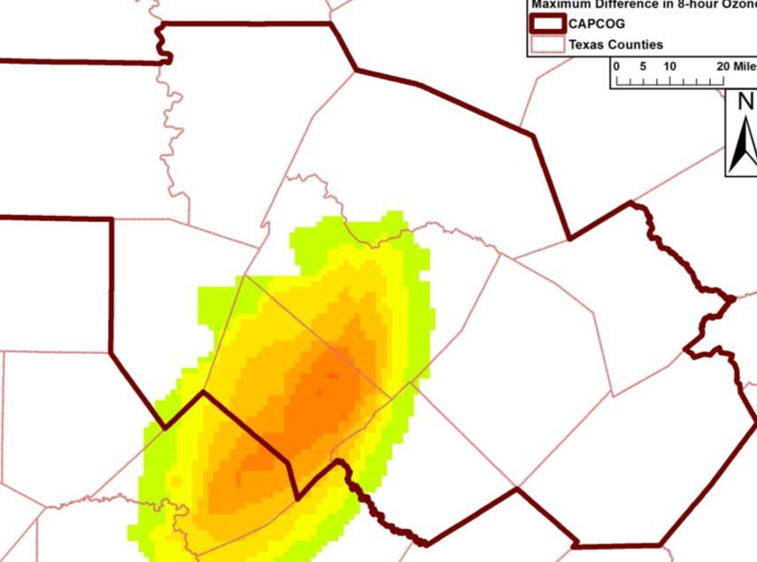
81 June 15 th June 27 th June 28 th June 29 th 3-8

82 June 30 th 3-9

83 3.3 Texas Lehigh Voluntary Ozone Action Day Photochemical Modeling Run The average impact of the change in hourly NO X reductions associated with Texas Lehigh s voluntary ozone action day program on peak 8-hour ozone concentrations on days > 70 ppb was a 0.02 ppb increase at C3 and a 0.03 ppb increase at C38 (Table 3-4). These increases may reflect the slightly higher NO X emissions before 9 am and after 3 pm on these days. For all days modeled from June 3-15 and from June 27-30, however, average 8-hour ozone levels decreased by 0.06 ppb at C3 and decreased by 0.03 ppb at C38. This difference may simply reflect the sensitivity of these results to the number of days included in the average, with the average across all days representing the more typical effect of the program on most days. The average change in peak 8- hour ozone in all grid cells on days > 60 ppb is ppb (Table 3-5). Table 3-6 shows the daily change in 8-hour ozone at each monitor. Ozone plots in Figure 3-2 show the change in ozone across the CAPCOG region due to Texas Lehigh s voluntary ozone action day program. On some days there was a slight increase in ozone at some locations in the CAPCOG region because of wind shifts in the model during these days. There is an increase in NO X emissions before 9 am at Texas Lehigh because of the voluntary program. On some days the wind direction in the early morning is towards the north which transports the increase NO X emissions towards the monitoring sites. After 8 am, the wind shifts to the southwest and the reductions in ozone is not recorded at the monitors north of Texas Lehigh. Table 3-4: Average Change in Peak 8-Hour Ozone at each Monitor for Texas Lehigh Voluntary Ozone Action Day Program, 2012 Photochemical Model Run Texas Lehigh Voluntary Ozone Action Day NOX Emission Reduction Program Monitor Change in Max 8-hour Ozone (ppb) Peak Days > 70 ppb All Days C C C C C C C C C

84 Table 3-5: Average Change in Peak 8-Hour Ozone in the 4km grid Covering the CAPCOG Region for Texas Lehigh Voluntary Ozone Action Day Program, 2012, (ppb). (Days > 60 ppb) Date Maximum peak 8- hour ozone across 10-county region Average peak 8-hour ozone average across 10-county region Average Daily Change (ppb) 3-Jun Jun Jun Jun Jun Jun Jun Jun Jun Jun Jun Jun Jun Jun Jun Jun Jun Average Change (Days > 60 ppb) Shaded rows are days were the predicted maximum ozone is not above 60 ppb 3-11

85 Table 3-6: Daily Change in Peak 8-Hour Ozone at each Monitor for Texas Lehigh Voluntary Ozone Action Day Program, ppb 2012 Monitor Run 3rd 4th 5th 6th 7th 8th 9th 10th 11th 12th 13th 14th 15th 27th 28th 29th 30th C3 C38 C614 C684 C690 C1603 C1604 C1675 Base Case Lehigh Base Case Lehigh Base Case Lehigh Base Case Lehigh Base Case Lehigh Base Case Lehigh Base Case Lehigh Base Case Lehigh Base Case C6602 Lehigh Based on peak 8-hour ozone in the 7x7 4km grids around each monitor Peak Days over 70 ppb in baseline are bolded 3-12

86 Figure 3-2: Difference in Maximum Ozone from Texas Lehigh Voluntary Ozone Action Day NO X Emission Reduction Program, ppb June 3 rd June 4 th June 5 th June 6 th 3-13

87 June 7 th June 8 th June 9 th June 10 th 3-14

88 June 11 th June 12 th June 13 th June 14 th 3-15