SAP-2010-FAQs-update.pdf

Transcription

1 ATM 507 Lecture 10 Text reading Section 5.7 Problem Set # 4 due Oct. 23 Midterm Oct. 25? Today s topics Polar Ozone, Global Ozone Trends Required reading: 20 Questions and Answers from the 2010 WMO report on Ozone Depletion: SAP-2010-FAQs-update.pdf 1

2 Recap 1. PSC formation esp. Type II with large particles that remove gaseous HNO Reactions on PSCs that remove NO x and liberate active ClO X. 3. Cl 2, HOCl, and ClNO 2 photolyze rapidly when the sun returns. 4. NO X buffers the release of active ClO X by forming ClNO 3, which in turn reacts with PSCs to form active ClO x and HNO When air is denitrified, active ClO x builds up and large scale O 3 depletion occurs via ClO + ClO, ClO + BrO, etc. 2

3 Schematic time series of chlorine and temperature in polar ozone depletion period. 3

4 Final comments Chemical models now include both gas phase and heterogeneous processes and do a reasonable job of describing polar ozone loss. ClO dimer mechanism accounts for up to 60-80% of the polar ozone loss ClO-BrO mechanism is the next biggest contributor There are outstanding problems (recall Stratospheric warming and 2002). Heterogeneous chemistry in the global stratosphere is an area of active research. Natural stratospheric aerosols Aircraft emissions Volcanoes 4

5 Q & A on Stratospheric Ozone 20 Questions and Answers from the 2010 WMO report on Ozone Depletion: SAP-2010-FAQs-update.pdf Required reading this may show up on the midterm! 5

6 From the 1998 Q&A set. 6

7 Ozone Trend Analysis Measurements of the total ozone column from ground stations and from satellites have been analyzed for trends in ozone. Some of the confounding factors include: The annual cycle Quasi-biennial oscillation (QBO) El Nino Southern Oscillation (ENSO) The 11 year solar cycle Volcanic eruptions Indications are, that on a global scale, ozone had decreased about 3% from Little change (slight increase?) since then. 7

8 Ground-Based Ozone Trend 8

9 Trend reversal? 9

10 Satellite Ozone Trend notice time range 10

11 Trend by Latitude and Season 11

12 Trends from Three Sets of Measurements 12

13 2006 Assessment Report 13

14 More sophisticated analysis from the 2006 Assessment EESC Effective Equivalent Stratospheric Chlorine 14

15 Ozone Assessments Scientific Assessment of Ozone Depletion World Meteorological Organization (WMO) 2010: _asst_report.html 2006: _asst_report.html 2002: _2002.html 1998: : 1991: 1989: Atmospheric Ozone:

16 From the Ozone Assessments TOTAL COLUMN OZONE 2002: Global mean total column ozone for the period was approximately 3% below the average. Since systematic global observations began, the lowest annually averaged global total column ozone occurred in (about 5% below the pre-1980 average). These changes are evident in each available global dataset Assessment: The decline in abundances of extrapolar stratospheric ozone seen in the 1990s has not continued. 2002: No significant trends in total column ozone have been observed in the tropics (25 N-25 S) for A decadal variation of total column ozone (with peak-to-trough variations of ~3%) is observed in this region, approximately in phase with the 11-year solar cycle. Total column ozone trends become statistically significant in the latitude bands in each hemisphere Assessment: No change from this conclusion. 16

17 2006 Assessment: Observations together with model studies suggest that the essentially unchanged column ozone abundances averaged over 60 S-60 N over roughly the past decade are related to the near constancy of stratospheric ozone-depleting gases during this period. 17

18 From the 2010 Assessment TOTAL COLUMN OZONE 2010: Average total ozone values in have remained at the same level for the past decade, about 3.5% and 2.5% below the averages respectively for 90 S-90 N and 60 S-60 N. 2010: The latitude dependence of simulated total column ozone trends generally agrees with that derived from measurements, showing large negative trends at Southern Hemisphere mid and high latitudes and Northern Hemisphere midlatitudes for the period of ODS (ozone depleting substances) increase. 18

19 POLAR OZONE (2006 Assessment) Springtime polar ozone depletion continues to be severe in cold stratospheric winters. Meteorological variability has played a larger role in the observed variability in ozone, over both poles, in the past few years. Large Antarctic ozone holes continue to occur. The severity of Antarctic ozone depletion has not continued to increase since the late 1990s and, since 2000, ozone levels have been higher than in some preceding years. These recent changes, seen to different degrees in different diagnostic analyses, result from increased dynamical activity and not from decreases in ozone-depleting substances. The Antarctic ozone hole now is not as strongly influenced by moderate decreases in ozonedepleting gases, and the unusually small ozone holes in some recent years (e.g., 2002 and 2004) are attributable to dynamical changes in the Antarctic vortex. The anomalous Antarctic ozone hole of 2002 was manifested in a smaller ozone-hole area and much smaller ozone depletion than in the previous decade. This anomaly was due to an unusual major stratospheric sudden warming. Arctic ozone depletion exhibits large year-to-year variability, driven by meteorological conditions. Over the past four decades, these conditions became more conducive to severe ozone depletion because of increasingly widespread conditions for the formation of polar stratospheric clouds during the coldest Arctic winters. This change is much larger than can be expected from the direct radiative effect of increasing greenhouse gas concentrations. The reason for the change is unclear, and it could be because of long-term natural variability or an unknown dynamical mechanism. The change in temperature conditions has contributed to large Arctic ozone losses during some winters since the mid-1990s. The Arctic winter 2004/2005 was exceptionally cold, and chemical ozone loss was among the largest ever diagnosed. The Arctic remains susceptible to large chemical ozone loss, and a lack of understanding of the long-term changes in the occurrence of polar stratospheric clouds limits our ability to predict the future evolution of Arctic ozone abundance and to detect the early signs of recovery. The role of chemical reactions of chlorine and bromine in the polar stratosphere is better quantified. Inclusion of these advances results in improved agreement between theory and observation of the timing of both Arctic and Antarctic polar ozone loss. 19

20 POLAR OZONE (2010 Assessment) The Antarctic ozone hole continued to appear each spring from 2006 to This is expected because decreases in stratospheric chlorine and bromine have been moderate over the last few years. Analysis shows that since 1979 the abundance of total column ozone in the Antarctic ozone hole has evolved in a manner consistent with the time evolution of ODSs. Since about 1997 the ODS amounts have been nearly constant and the depth and magnitude of the ozone hole have been controlled by variations in temperature and dynamics. The October mean column ozone within the vortex has been about 40% below 1980 values for the past fifteen years. Arctic winter and spring ozone loss has varied between 2007 and 2010, but remained in a range comparable to the values that have prevailed since the early 1990s. Chemical loss of about 80% of the losses observed in the record cold winters of 1999/2000 and 2004/2005 has occurred in recent cold winters. Recent laboratory measurements of the chlorine monoxide dimer (ClOOCl) dissociation cross section and analyses of observations from aircraft and satellites have reaffirmed the fundamental understanding that polar springtime ozone depletion is caused primarily by the ClO + ClO catalytic ozone destruction cycle, with significant contributions from the BrO + ClO cycle. Polar stratospheric clouds (PSCs) over Antarctica occur more frequently in early June and less frequently in September than expected based on the previous satellite PSC climatology. This result is obtained from measurements by a new class of satellite instruments that provide daily vortex-wide information concerning PSC composition and occurrence in both hemispheres. The previous satellite PSC climatology was developed from solar occultation instruments that have limited daily coverage. Calculations constrained to match observed temperatures and halogen levels produce Antarctic ozone losses that are close to those derived from data. Without constraints, CCMs simulate many aspects of the Antarctic ozone hole, however they do not simultaneously produce the cold temperatures, isolation from middle latitudes, deep descent, and high amounts of halogens in the polar vortex. Furthermore, most CCMs underestimate the Arctic ozone loss that 20 is derived from observations, primarily because the simulated northern winter vortices are too warm.

21 21

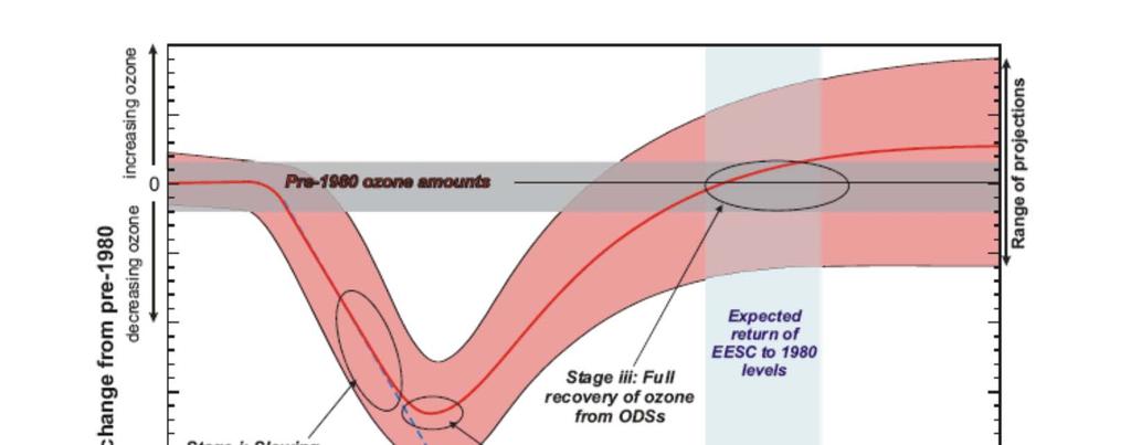
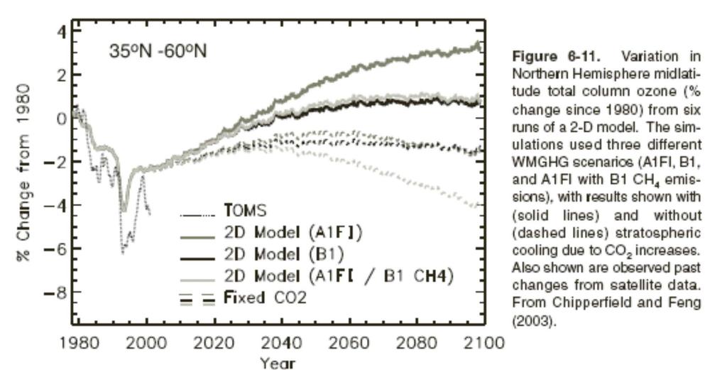
22 Measurements plus Projections 22

23 23

24 Trends and Predictions Note the large dip in the early 1990 s this led to overly high projections of ozone loss until the 1998 assessment. The extra loss is thought to be due to the effects of the Pinatubo volcano. Recovery (timing and magnitude) depends on emissions scenarios. 24

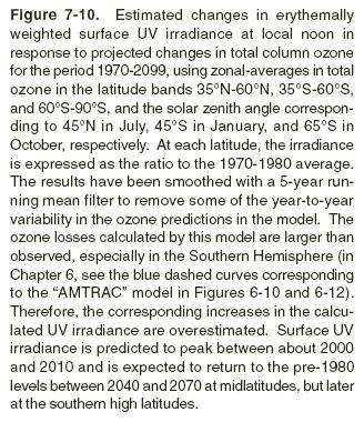
25 Linkage of Ozone and UV Radiation Less ozone means more UV at the Earth s surface. Analysis of this trend is also very important. Effect is not linear, but for small changes in the ozone column it can be approximated as linear. 25

26 Relation between ozone and UV changes Dependence of erythemal ultraviolet (UV) radiation at the Earth's surface on atmospheric ozone, measured on cloud-free days at various locations, at fixed solar zenith angles. Legend: South Pole (Booth and Madronich, 1994); Mauna Loa, Hawaii (Bodhaine et al., 1997); Lauder, New Zealand (McKenzie et al., 1998); Thessaloniki, Greece (updated from Zerefos et al., 1997); Garmisch, Germany (Mayer et al., 1997); and Toronto, Canada (updated from Fioletov et al., 1997). Solid curve shows model prediction with a power rule using RAF =

27 Radiation Amplification Factor (RAF) Radiation Amplification Factor (RAF) is defined as the percentage increase in UV bio that would result from a 1% decrease in the column amount of atmospheric ozone. The radiation amplification factors are given in for a number of different known effects. The RAFs can generally be used only to estimate effects of small ozone changes, e.g. of a few percent, because the relationship between ozone and UV bio becomes non-linear for larger ozone changes. 27

28 Trends in biologically active UV from TOMS ( ) - increasing. Latitude band - degrees Trend (a) - % per decade Uncertainty (b) ±2 sigma 70 S 60 S S 50 S S 40 S S 30 S S 20 S S 10 S S N N 20 N N 30 N N 40 N N 50 N N 60 N N 70 N Trends in biologically active radiation (weighted with the erythemal action spectrum of McKinlay and Diffey, 1987), derived from total ozone and cloud reflectivity measurements from the Total Ozone Mapping Spectrometer (TOMS, version 7) over Adapted from Herman et al. (1996). (a) Zonally averaged trend over given latitude band, values rounded to nearest half percent. (b) As corrected by Herman et al. (1998) and includes combined instrumental error and variability of 28 UV radiances.

29 29

30 30

31 Also from Ozone Assessment Ground-based UV reconstructions and satellite UV retrievals, supported in the later years by direct ground-based UV measurements, show that erythemal ("sunburning") irradiance over midlatitudes has increased since the late 1970s, in qualitative agreement with the observed decrease in column ozone. The increase in satellite-derived erythemal irradiance over midlatitudes during is statistically significant, while there are no significant changes in the tropics. Satellite estimates of UV are difficult to interpret over the polar regions. In the Antarctic, large ozone losses produce a clear increase in surface UV radiation. Ground-based measurements show that the average spring erythemal irradiance for is up to 85% greater than the modeled irradiance for , depending on site. The Antarctic spring erythemal irradiance is approximately twice that measured in the Arctic for the same season. Clear-sky UV observations from unpolluted sites in midlatitudes show that since the late 1990s, UV irradiance levels have been approximately constant, consistent with ozone column observations over this period. Surface UV levels and trends have also been significantly influenced by clouds and aerosols, in addition to stratospheric ozone. Daily measurements under all atmospheric conditions at sites in Europe and Japan show that erythemal irradiance has continued to increase in recent years due to net reductions in the effects of clouds and aerosols. In contrast, in southern midlatitudes, zonal and annual average erythemal irradiance increases due to ozone decreases since 1979 have been offset by almost a half due to net increases in the effects of clouds and aerosols. 31

32 Chemical Models of the Stratosphere Concepts of atmospheric models (as applied to the lower atmosphere) are presented in Chapter 25 Models needed for understanding past and present; and for predicting future outcomes. Future outcomes depend on emission scenarios. Source gas emissions for the stratosphere are better understood than those for the troposphere. 32

33 Models (cont.) Models include 1. Reaction Rate Coefficients 2. Photolysis Rate Coefficients (these vary with solar flux, i.e., SZA, ozone, aerosol, albedo) 3. Initial conditions for species and meteorological quantities (p, T, [species], ) 4. Met forecast model or parameterization of transport (including fluxes of source gases to the stratosphere) 5. Treatment of heterogeneous chemistry and physics Types of calculations 1. Steady-State Calculation: Fixed inputs, run until stable outputs 2. Prognostic Calculation: Estimate changes in inputs (chemical, solar, transport) and run model to predict or project possible outcomes 33

34 Types of Models 0-D or box model: only variable is time 1-D model: Vary time and altitude (vertical transport is estimated using eddy diffusion ) 2-D model: vary time, altitude, and latitude (transport estimated with 2x2 matrix of transport coefficients) 3-D model: becoming more common, but resolution is quite coarse in many cases, and requires greater computer resources. Usually coupled with met model. 34

35 Ozone Depletion Potential Start with an Ozone Depletion Model Reference Species is CFCl 3 (CFC-11 or Freon 11). All other ozone depleting species (mostly chlorine and bromine containing compounds) are compared to CFC-11. Properties of CFC-11 (CFCl 3 ): 3 Cl atoms per molecule Unreactive in troposphere, so it is (eventually) transported to the stratosphere, where its lifetime with respect to photolysis is ~45 years It is photolyzed in the stratosphere to yield Cl atoms Chlorine catalyzed ozone destruction occurs in polar regions and in midlatitudes (different mechanisms) 35

36 Ozone Depletion Potential (cont.) BY DEFINITION ODP OF CFC-11 = 1. The ODP is a property of the species. All other species ODP s are referenced to the ODP of CFC-11. Consider HCFC-22 HCFC-22 = CHF 2 Cl (= X in our example) Properties of HCFC-22: 1 Cl atom per molecule Reacts slowly in the troposphere (chemical lifetime ~12 years) If it penetrates into the stratosphere, it can be photolyzed to release Cl and destroy O 3. 36

37 Methods of Calculating ODP Better (but computationally more difficult) method 1. Find the emission rate of CFC-11 (kg/yr) that results in a 1% O 3 depletion. Call this emission rate A. 2. Find the emission rate of compound X (kg/yr) that results in a 1% O 3 depletion. Call this emission rate B. 3. ODP of X = A/B. More practical (but less rigorous) method 1. Calculate ΔO 3 per unit mass emission rate of CFC- 11. Call this ΔO 3 A. 2. Calculate ΔO 3 per unit mass emission rate of compound X. Call this ΔO 3 B. 3. ODP of X = B /A. 37

38 GLOBALLY AVERAGED ODP Ozone Depletion Potential ODP = ΔO ΔO z z Θ Θ t t 3 3 ( z, Θ, t) ( z, Θ, t) for X for CFC 11 cosθ cosθ z = altitude, Θ = latitude, t = time ΔO 3 = change in O 3 at steady state (per unit mass emission rate) Examples of global ODP s HCFC -22 ODP = HCFC-142b (CH 3 CF 2 Cl) ODP = CH 3 CCl 3 ODP = 0.13 CF 3 Br (H-3101) ODP = NOTE: Local ODP s vary greatly (e.g. Polar Spring) 38

39 Trends of Controlled Ozone Depleting Chemicals 39

40 EECl = Effective Equivalent Chlorine (as Cl 2 ) 40

41 The factor of two difference in the scale on this slide compared to the last one comes about because Cl 2 contains two Cl atoms. 41